HAL Id: hal-00296944
https://hal.archives-ouvertes.fr/hal-00296944
Submitted on 20 Feb 2006
HAL is a multi-disciplinary open access
archive for the deposit and dissemination of
sci-entific research documents, whether they are
pub-lished or not. The documents may come from
teaching and research institutions in France or
abroad, or from public or private research centers.
L’archive ouverte pluridisciplinaire HAL, est
destinée au dépôt et à la diffusion de documents
scientifiques de niveau recherche, publiés ou non,
émanant des établissements d’enseignement et de
recherche français ou étrangers, des laboratoires
publics ou privés.
ENSO impact on simulated South American
hydro-climatology
J. Stuck, A. Güntner, B. Merz
To cite this version:
J. Stuck, A. Güntner, B. Merz. ENSO impact on simulated South American hydro-climatology.
Advances in Geosciences, European Geosciences Union, 2006, 6, pp.227-236. �hal-00296944�
Advances in Geosciences, 6, 227–236, 2006 SRef-ID: 1680-7359/adgeo/2006-6-227 European Geosciences Union
© 2006 Author(s). This work is licensed under a Creative Commons License.
Advances in
Geosciences
ENSO impact on simulated South American hydro-climatology
J. Stuck, A. G ¨untner, and B. Merz
GeoForschungsZentrum Potsdam (GFZ), Telegrafenberg, 14473 Potsdam, Germany
Received: 7 November 2005 – Revised: 15 December 2005 – Accepted: 21 December 2005 – Published: 20 February 2006
Abstract. The variability of the simulated hydro-climatology of the WaterGAP Global Hydrology Model (WGHM) is analysed. Main object of this study is the ENSO-driven variability of the water storage of South Amer-ica. The horizontal model resolution amounts to 0.5 degree and it is forced with monthly climate variables for 1961– 1995 of the Tyndall Centre Climate Research Unit dataset (CRU TS 2.0) as a representation of the observed climate state. Secondly, the model is also forced by the model out-put of a global circulation model, the ECHAM4-T42 GCM. This model itself is driven by observed monthly means of the global Sea Surface Temperatures (SST) and the sea ice coverage for the period of 1903 to 1994 (GISST). Thus, the climate model and the hydrological model represent a re-alistic simulated realisation of the hydro-climatologic state of the last century. Since four simulations of the ECHAM4 model with the same forcing, but with different initial con-ditions are carried out, an analysis of variance (ANOVA) gives an impression of the impact of the varying SST on the hydro-climatology, because the variance can be separated into a SST-explained and a model internal variability (noise). Also regional multivariate analyses, like Empirical Orthog-onal Functions (EOF) and Canonical Correlation Analysis (CCA) provide information of the complex time-space vari-ability. In particular the Amazon region and the South of Brazil are significantly influenced by the ENSO-variability, but also the Pacific coastal areas of Ecuador and Peru are af-fected. Additionally, different ENSO-indices, based on SST anomalies (e.g. NINO3.4, NINO1+2), and its influence on the South American hydro-climatology are analysed. Espe-cially, the Pacific coast regions of Ecuador, Peru and Chile show a very different behaviour dependant on those indices.
Correspondence to: J. Stuck
1 Introduction
The South American hydro-climatology is highly affected by positive (El Ni˜no) and negative (La Ni˜na) events of the El Ni˜no Southern Oscillation (ENSO) in various ways (e.g. Ro-pelewski and Halpert (1987), Aceituno (1988), Vuille (1999), Waylen and Poveda (2002)). In some studies relative high correlations between ENSO and the river discharge of the most important South American rivers, the Amazon and the Paran´a were found (Richey et al. (1989), Amarasekera et al. (1997)). Those ENSO-forced variations are accompanied by ecological and economical consequences, in particular in the Pacific coastal areas of Ecuador, Peru and Chile (e.g. Glynn (1990), Waylen and Poveda (2002)), but also in most other parts of South America. Thus, it is of considerable value to improve the knowledge of the ENSO impact on the South American hydro-climatology.
Since ENSO prediction has been improved in the last decade and reliable prognostics of the occurence of an ENSO event are possible, at least three to six months in advance, also most of the prominant variations in river discharge and water storage are predictable, if they are generally well-known by previous analyses of available data. But most of those variations are only locally well-known (e.g. river dis-charge, lake level variations). In particular, observations of the water storage are not available at least for large areas. But quantifying just these water storage variations is of high importance for applications where the water availability in terms of water storage is required, for instance as soil mois-ture for evapotranspiration, or as water storage for human consumption, or for assessing the effect of land water stor-age on the global sea level (Ngo-Duc et al., 2005).
Since recently, a new data source is available to estimate the water storage variations from remote sensing. The satel-lite mission of the “Gravity Recovery and Climate Experi-ment” (GRACE) was launched in march 2002 (Tapley et al., 2004a). It provides temporal mass variations by monitoring the time-varying gravity field of the Earth. These variations correspond to the water storage changes after correcting for
228 Stuck et al.: ENSO impact on South American hydro-climatology mass variations of the solid Earth, the atmosphere and the
ocean.
First results of the GRACE mission show, that the accu-racy is high enough to be of value for hydrological applica-tions, resolving interannual (Andersen and Hinderer, 2005) and seasonal water storage variations (Wahr et al. (2004), Tapley et al. (2004b), Schmidt et al. (2005), Ramillien et al. (2005)) for large regions and river basins. These re-sults show, that the seasonal water storage variations in South America are one of the largest worldwide. They occur mainly in Northern parts of South America including the Amazon and the Orinoco basin. As this region is also highly af-fected by ENSO, a strong interannual signal of water stor-age changes can be expected, which also may be visible by GRACE in terms of variations of the gravity field.
In a second focus of our analysis is the Pacific coast region including Peru and Chile. This is constituted by the CEN-SOR1project. The aim of our analyses is the estimation of the ENSO impact on the freshwater and sediment input into the coastal areas of Peru and Chile, for which water storage is an important boundary condition.
This study should give a first impression of the ENSO im-pact on the large scale South American hydro-climatology simulated with a global hydrological model. The typical modes of the ENSO-driven variability should be detected with an additional focus on the Pacific coast region of Peru and Chile.
2 Methodology and models
In this study the analysis is performed with the Water-gap Global Hydrology Model (WGHM; D¨oll et al. (2003)), which is a simple conceptual model of the continental hy-drological cycle. It represents the main water storage com-ponents like soil water, groundwater, water storage as snow and ice, and, finally, surface water storage, in rivers, lakes, reservoirs, and water storage in wetlands and other inundated areas. For more details regarding model physics see D¨oll et al. (2003).]
The horizontal resolution of the WGHM amounts to 0.5◦×0.5◦latitude-longitude and it works with a timestep of one day. The model is forced with different kind of climato-logical datasets of monthly means of precipitation, temper-ature (2 m), short wave radiation and the cloud cover. On the one hand the forcing fields are derived from the Cli-mate Research Unit (CRU-) dataset covering the time period from 1901 to 1995 with the same horizontal resolution as the WGHM (New et al., 2000). The analyses are restricted only to subset of the data for the time period from 1961 to 1995, because the quality of the CRU dataset, and as a consequence the model output, are worse before at least 1950. That means, the required stationarity of the data for linear statistics would not be given, using the whole time period. It should also be 1Climate variability and El Ni˜no Southern Oscillation:
impli-cations for natural coastal resources and management (http://www. censor.name).
mentioned, that due to the lack of observational data in many parts of South America, the CRU-dataset gives not a perfect representation of the climate state.
On the other hand the data stem from an ensemble of the ECHAM4-T42 global circulation model (Roeckner et al., 1996), which was developed at the Max Planck Institute for meteorology (MPI). This model was forced with anal-ysed observations of the monthly mean Sea Surface Tem-peratures (SST) and the global Ice coverage (GISST dataset) performed by the Hadley center (Rayner et al., 1996). This forcing covers the time period from 1903 to 1994 (recently to 2002) and 4 simulations with different initial conditions were carried out. Indeed, the forcing fields of the ECHAM4 model with a horizontal resolution of 2.8◦, due to the
spec-tral T42 representation, are coarse compared to the CRU-dataset, but those simulated atmospheric data are consis-tent in time, while the reliability of the CRU-data is time-dependant. Additionally, the signal-to-noise ratio will be improved by analysing the ensemble mean of the 4 simu-lations. Since the signal of the ENSO is represented by SST anomalies, the impact of the ENSO on the simulated hydro-climatology is more pronounced in respect to the natural vari-ability. That means, the detection of a typical ENSO signal will be more probable.
The analysis of the ENSO impact on the South Amer-ican hydro-climatology includes the Analysis of Vari-ance (ANOVA; Rowell et al. (1995)), multivariate statis-tics like Principal Component Analysis (Kutzbach (1967), Preisendorfer (1988), von Storch and Zwiers (1999)), Canon-ical Correlation Analysis (CCA; Bretherton et al. (1992)) and a time-frequency analysis with the Wavelet Transformation (Torrence and Compo, 1998). This analyses are common tools in the multivariate statistics and time series analysis and should not be explained in detail in this paper.
3 South American hydro-climatology
To analyse the linear part of the response of the ENSO on the South American hydro-climatology with the help of the ANOVA, the same amount of positive and negative events must be defined. We found 12 La Ni˜na (cold) events and 12 El Ni˜no (warm) events by means of the NINO3.4 index time series from 1903 to 1994, even though there are more warm events than cold events in this period. Thus, weaker El Ni˜no years are not considered to conserve the equilibrium between both extremes. To compare the results of the ENSO “treatment” with neutral conditions, we have also defined 24 typical Non-ENSO years by means of the NINO3.4 index series.
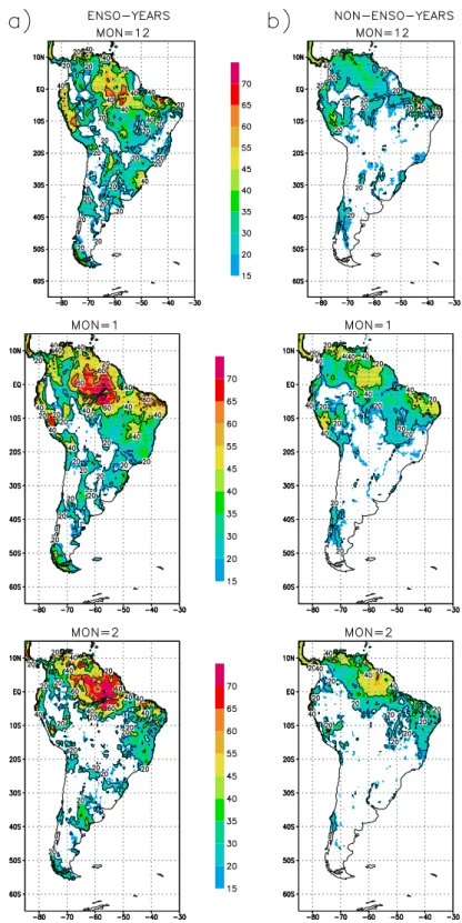
Figure 1 shows the results of the ANOVA, the explained variance of the simulated total water storage, for the boreal winter months december (mon=12), january (mon=1) and february (mon=2) in ENSO years (upper panel) and Non-ENSO years (lower panel). It is obvious, that the explained (SST-forced) variance in ENSO years reaches higher values in most parts of South America than in Non-ENSO years. In
Stuck et al.: ENSO impact on South American hydro-climatology
Stuck et al.: ENSO impact on South American hydro-climatology
2293
Fig. 1. ANOVA of the simulated total water storage in ENSO years
a) and in Non-ENSO years b) in the boreal winter months decem-ber (mon=12) of the ENSO (Non-ENSO) defined year, and january (mon=1) and february (mon=2) of the following year, respectively. Shaded contours are significant explained variance (contour inter-vall: 5%).
Non-ENSO years the values reach only 45%. At the coastal
areas of Ecuador and Northern Peru there are also high
val-ues with 60% explained variance in ENSO years in contrast
to lower values in neutral years. The relative high values of
45%
in Non-ENSO years in the amazon basin are not very
surprising since the precipitation there is also dependant on
the SST of the tropical atlantic (e.g. Enfield (1996), Fu et al.
(2001)).
The higher values of explained variance in some regions in
ENSO years show that the simulated variability of the water
storage is enhanced in those years. That means the impact
of El Ni˜no and La Ni˜na is contrary, as expected, at least in a
linear way of thinking. To detect also a qualitative response
of the ENSO on the water storage we have applied a
canon-ical correlation analysis (CCA). The CCA in this study is
performed with a reduction of the degrees of freedom by
us-ing a basis of Empirical Orthogonal Functions (EOF) after
Bretherton et al. (1992). Those EOF represent the dominant
space-time variability of the variate (e.g. the water storage)
and the corresponding amplitudes describe the evolution of
the EOF with time. Thus, before interpreting the variability
patterns of the CCA we consider the patterns of the
domi-nant EOF. Certainly the seasonal variations are excluded by
removing the long term monthly means.
The 1.EOF (Fig. 2) of the water storage of the
ensem-ble mean of the ECHAM4-forced simulations explains more
than a quarter (26, 2%) of the total variability. The pattern
shows maximum variations in the Northern and Central parts
of Brazil with maximum values in the Northeast. The coastal
and west andean region of Peru and Northern Chile offers
positive anomalies of the water storage as well, while most
of the Southern parts of South America show negative
varia-tions with the exception of the Paran´a river and Patagonia.
This variability mainly represents interannual and decadal
variations of the South American water storage, which is
shown by the Wavelet Power spectrum of the corresponding
amplitude of the EOF (Fig. 2, right panel). It has a significant
variability in the 1980’ies, starting with the El Ni˜no event of
1982/83, and also in the 1920’ies and 1930’ies with a
pe-riod of approximately 5 years. But the spectrum shows also
a permanent signal around periods of 10 to 15 years over
the whole time-frame with a 5% significance at the end of
the time series. This coexistence of interannual and decadal
variations suggests an influence of the ENSO, but also,
per-haps, of its decadal modulation, the Pacific Decadal
Oscil-lation (PDO, Zhang et al. (1997)). This is confirmed by the
work of Cobb et al. (2001) as well. They found a
signifi-cant correlation between central tropical Pacific SST (corals)
and rainfall in North-Eastern Brazil with periods of 12-13
years. The 2.EOF (not shown) did not represent a typical
ENSO response, either. Thus, the continental scale
variabil-ity of South America is certainly not only influenced by the
ENSO, but some typical regional coherencies are already be
identified by the 1.EOF.
The 1.EOF of the CRU-forced simulated water storage (Fig.
3) shows a very different pattern compared to the
ECHAM-forced EOF. The pattern of the 1.EOF shows predominantly
a dipole structure of the anomalies of the water storage with
positive values in the Northern part of South America, which
peaks in the Amazon river with anomalies of 400 mm water
equivalent, and negative anomalies in the Southern part. It
explains similarly a quarter (24.3%) of the total variability of
the simulated water storage, but there is no typical allocation
in the time-frequency domain (Fig. 3, right panel). Only in
1982/83 a significant signal in the amplitude of the 1.EOF
with a period of 2 years is coherent with the well-known El
Ni˜no event. Such a phase relation between the ENSO and
Fig. 1. ANOVA of the simulated total water storage in ENSO years a) and in Non-ENSO years b) in the boreal winter months december (mon=12) of the ENSO (Non-ENSO) defined year, and january (mon=1) and february (mon=2) of the following year, respectively. Shaded contours are significant explained variance (contour intervall: 5%).
particular in january and february the values exceed an ex-plained variance of 70% in North-Eastern Brazil, while in Non-ENSO years the values reach only 45%. At the coastal areas of Ecuador and Northern Peru there are also high
val-ues with 60% explained variance in ENSO years in contrast to lower values in neutral years.
230
4
Stuck et al.: ENSO impact on South American hydro-climatologyStuck et al.: ENSO impact on South American hydro-climatology
Fig. 2. 1.EOF of the South American total water storage of the
en-semble mean of 4 simulations forced with ECHAM4 (1903-1994),
contours are mm water equivalent. The right panel show the wavelet
power spectrum of the amplitude of the EOF pattern. Contours are
multiple of the variance, black solid line represents 5% significance
level.
Fig. 3. same as fig. 2 but for the CRU forcing (1961-1995)
a 2-year signal in climate variates is also well known, but it
originates from the stratospheric Quasi Biennial Oscillation
(QBO, Gray et al. (1992)) or from the Tropospheric Biennial
Oscillation (TBO, Meehl (1987)). Since those variations are
focused either on the stratosphere or on the Western Pacific
and Asia, it is improbable, that this 2-year signal of the South
American hydro-climatology is linked to those TBO or QBO.
That difference between the EOF of the CRU-forced model
run and the EOF of the ensemble mean of the
ECHAM-forced runs is not surprising, since the signal-to-noise ratio
is improved by the constitution of the ensemble mean and
since the underlying time period of both simulations is
dif-ferent. But also the comparison with only one single run (not
shown) shows few coincidencies with the CRU-forced EOF.
Thus, a simple principal component analysis is not able
to detect the typical ENSO impact on the simulated South
American water storage variations. Now, a canonical
corre-lation analysis (CCA) shall provide the ENSO signal on the
water storage variability of South America. Therefore we
have used the Pacific SST (60
oS - 60
oN, 120
oE - 70
oW) from
the GISST dataset, which are used to force the ECHAM4
simulations, and the simulated grid cell data of the total
wa-ter storage. This CCA maximises the linear relationship of
two variates.
The analysis is applied to the ensemble mean of the
simu-lated total water storage of the ECHAM-forced runs (4a) and
to one single ECHAM-forced simulation alone (4b). The first
canonical correlation patterns of the ensemble mean
analy-sis yields a SST variability, which describes the typical SST
anomaly of an El Ni˜no event. The maximum canonical
cor-related (0.81) water storage variation pattern of the
ensem-ble mean shows most of the expected anomalies as far as
they are expectedly. Due to the well known strong increased
precipitation in the coastal areas of Ecuador and Peru the
water storage offers positive anomalies in these areas when
the SST anomaly peaks in boreal winter. Likewise the
pat-tern consists of positive anomalies in central Chile,
South-ern Brazil and NorthSouth-ern Argentina. Decreased water storage
can be found in Southern Peru and Northern Chile and in
the Amzon basin in the North of Brazil as well. Most of
these areas are also detected by the ANOVA (Fig. 1) by
sig-nificantly explained variance of the water storage in ENSO
years. The spectral behaviour of the amplitude of the SST
and the water storage is presented by the wavelet power
spec-trum (Fig. 5a) and shows the typical variations of the ENSO.
The spectrum looks absolutely the same as the spectrum of a
SST-based ENSO index series like NINO3 or NINO3.4 (e.g.
Torrence and Compo (1998), their Fig. 1b), which confirms
the assumption, that these CCA patterns represent the typical
ENSO variability.
The same analysis, with only one realisation of the
ECHAM-forced model run, shows a similar pattern of SST
variations for the 1.CCA mode (Fig. 4b). But anyhow those
variations represent a complete different mode of
variabil-ity. For example, the pattern shows no SST anomalies off the
South American Pacific coast, where usually the strongest
SST anomalies of an ENSO event occur. The amplitude of
this CCA pattern gives no hint for a linkage with the ENSO.
It consists of a nearly decadal signal between 1940 and 1960
and some weak interannual signals in the same period and in
the 1980ies (Fig.5b). But all of these signals are not
signif-icant at the 5% level. Accordingly, the corresponding total
water storage variations did not display any typical
ENSO-caused variation. The same holds for the CCA analysis using
the CRU-forced simulated water storage (not shown). The
maximum canonical correlation did not bring out the
typ-ical ENSO variations. This emphasizes clearly the
advan-tage of the constitution of the ensemble mean. With the
im-provement of the signal-to-noise ratio the signal is detectable,
but on the other hand, the signal is that weak, that it isn’t
detectable in one realisation of the South American
hydro-climatology alone. This is attributed to the complex
space-time structure or rather the non-linear behaviour of the
pre-cipitation and the water storage as well.
To focus on the regional scale, a correlation and regression
analysis is performed for the tropical and subtropical Pacific
coast area. The typical ENSO indices are univariate
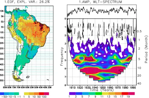
corre-Fig. 2. 1.EOF of the South American total water storage of the ensemble mean of 4 simulations forced with ECHAM4 (1903–1994), contoursare mm water equivalent. The right panel show the wavelet power spectrum of the amplitude of the EOF pattern. Contours are multiple of the variance, black solid line represents 5% significance level.
4
Stuck et al.: ENSO impact on South American hydro-climatology
Fig. 2. 1.EOF of the South American total water storage of the
en-semble mean of 4 simulations forced with ECHAM4 (1903-1994),
contours are mm water equivalent. The right panel show the wavelet
power spectrum of the amplitude of the EOF pattern. Contours are
multiple of the variance, black solid line represents 5% significance
level.
Fig. 3. same as fig. 2 but for the CRU forcing (1961-1995)
a 2-year signal in climate variates is also well known, but it
originates from the stratospheric Quasi Biennial Oscillation
(QBO, Gray et al. (1992)) or from the Tropospheric Biennial
Oscillation (TBO, Meehl (1987)). Since those variations are
focused either on the stratosphere or on the Western Pacific
and Asia, it is improbable, that this 2-year signal of the South
American hydro-climatology is linked to those TBO or QBO.
That difference between the EOF of the CRU-forced model
run and the EOF of the ensemble mean of the
ECHAM-forced runs is not surprising, since the signal-to-noise ratio
is improved by the constitution of the ensemble mean and
since the underlying time period of both simulations is
dif-ferent. But also the comparison with only one single run (not
shown) shows few coincidencies with the CRU-forced EOF.
Thus, a simple principal component analysis is not able
to detect the typical ENSO impact on the simulated South
American water storage variations. Now, a canonical
corre-lation analysis (CCA) shall provide the ENSO signal on the
water storage variability of South America. Therefore we
have used the Pacific SST (60
oS - 60
oN, 120
oE - 70
oW) from
the GISST dataset, which are used to force the ECHAM4
simulations, and the simulated grid cell data of the total
wa-ter storage. This CCA maximises the linear relationship of
two variates.
The analysis is applied to the ensemble mean of the
simu-lated total water storage of the ECHAM-forced runs (4a) and
to one single ECHAM-forced simulation alone (4b). The first
canonical correlation patterns of the ensemble mean
analy-sis yields a SST variability, which describes the typical SST
anomaly of an El Ni˜no event. The maximum canonical
cor-related (0.81) water storage variation pattern of the
ensem-ble mean shows most of the expected anomalies as far as
they are expectedly. Due to the well known strong increased
precipitation in the coastal areas of Ecuador and Peru the
water storage offers positive anomalies in these areas when
the SST anomaly peaks in boreal winter. Likewise the
pat-tern consists of positive anomalies in central Chile,
South-ern Brazil and NorthSouth-ern Argentina. Decreased water storage
can be found in Southern Peru and Northern Chile and in
the Amzon basin in the North of Brazil as well. Most of
these areas are also detected by the ANOVA (Fig. 1) by
sig-nificantly explained variance of the water storage in ENSO
years. The spectral behaviour of the amplitude of the SST
and the water storage is presented by the wavelet power
spec-trum (Fig. 5a) and shows the typical variations of the ENSO.
The spectrum looks absolutely the same as the spectrum of a
SST-based ENSO index series like NINO3 or NINO3.4 (e.g.
Torrence and Compo (1998), their Fig. 1b), which confirms
the assumption, that these CCA patterns represent the typical
ENSO variability.
The same analysis, with only one realisation of the
ECHAM-forced model run, shows a similar pattern of SST
variations for the 1.CCA mode (Fig. 4b). But anyhow those
variations represent a complete different mode of
variabil-ity. For example, the pattern shows no SST anomalies off the
South American Pacific coast, where usually the strongest
SST anomalies of an ENSO event occur. The amplitude of
this CCA pattern gives no hint for a linkage with the ENSO.
It consists of a nearly decadal signal between 1940 and 1960
and some weak interannual signals in the same period and in
the 1980ies (Fig.5b). But all of these signals are not
signif-icant at the 5% level. Accordingly, the corresponding total
water storage variations did not display any typical
ENSO-caused variation. The same holds for the CCA analysis using
the CRU-forced simulated water storage (not shown). The
maximum canonical correlation did not bring out the
typ-ical ENSO variations. This emphasizes clearly the
advan-tage of the constitution of the ensemble mean. With the
im-provement of the signal-to-noise ratio the signal is detectable,
but on the other hand, the signal is that weak, that it isn’t
detectable in one realisation of the South American
hydro-climatology alone. This is attributed to the complex
space-time structure or rather the non-linear behaviour of the
pre-cipitation and the water storage as well.
To focus on the regional scale, a correlation and regression
analysis is performed for the tropical and subtropical Pacific
coast area. The typical ENSO indices are univariate
corre-Fig. 3. same as corre-Fig. 2 but for the CRU forcing (1961–1995).The relative high values of 45% in Non-ENSO years in the amazon basin are not very surprising since the precipitation there is also dependant on the SST of the tropical atlantic (e.g. Enfield (1996), Fu et al. (2001)).
The higher values of explained variance in some regions in ENSO years show that the simulated variability of the water storage is enhanced in those years. That means the impact of El Ni˜no and La Ni˜na is contrary, as expected, at least in a lin-ear way of thinking. To detect also a qualitative response of the ENSO on the water storage we have applied a canonical correlation analysis (CCA).
The CCA in this study is performed with a reduction of the degrees of freedom by using a basis of Empirical Orthogonal Functions (EOF) after Bretherton et al. (1992). Those EOF represent the dominant space-time variability of the variate (e.g. the water storage) and the corresponding amplitudes describe the evolution of the EOF with time. Thus, before interpreting the variability patterns of the CCA we consider the patterns of the dominant EOF. Certainly the seasonal variations are excluded by removing the long term monthly means.
Stuck et al.: ENSO impact on South American hydro-climatology
Stuck et al.: ENSO impact on South American hydro-climatology
2315
Fig. 4. 1.CCA of the pacific SST (60
oS - 60
oN, 120
oE - 70
oW)
and the South American total water storage of the ensemble mean
of 4 simulations (a) and one single simulation (b). The right panel
show the wavelet power spectrum of the amplitude of the canonical
pattern, respectively.
lated with the water storage of Ecuador, Peru and Northern
Chile. Additionally a series of time lagged correlations is
constructed to demonstrate the evolution of the ENSO
cor-related anomalies of the water storage after the peak phase
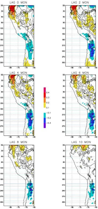
of an ENSO event. Figure 6 presents the correlation and
the regression of the water storage with the NINO3.4 index.
The water storage reflects mainly the typical precipitation
anomalies accompanied with an ENSO event. Significant
positive correlations occur in the coastal areas of Ecuador
and Northern Peru when the ENSO event peaks (lag 0) and
negative correlations can be found in Southern Peru, the
Altiplano, parts of the Atacama desert and North-West
Ar-gentina. While those negative correlations enhance and last
for at least 6 to 8 months, the positive anomalies in Ecuador
and Northern Peru decreases slowly with time. Only in the
central parts of Peru some weak but significant correlations
develop or last until a time lag of 6 months. The Ecuadorian
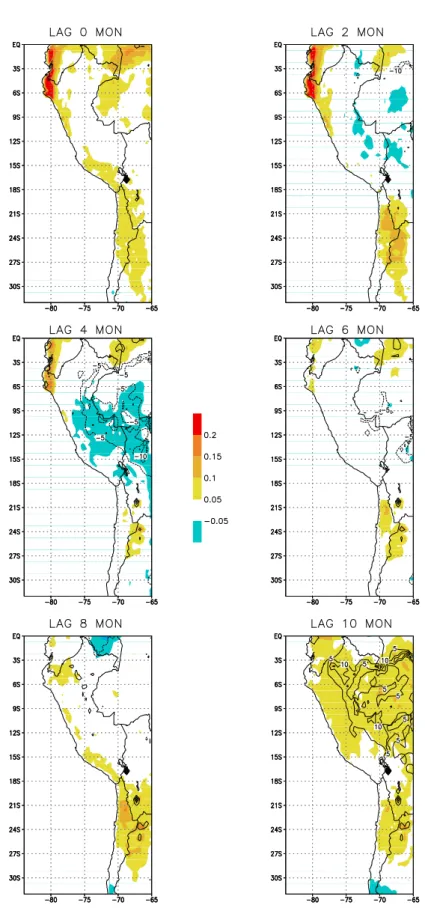
rainfall and as a result, the water storage is much higher
cor-related to SST anomalies off the Pacific coast (NINO1+2), as
it is highlighted by the difference of correlation of the water
storage with the NINO1+2 and the NINO3.4 region (Fig. 7).
The higher correlation with increased coefficients up to more
than 0.2 is concentrated only on the coastal line. This
differ-Fig. 5. Wavelet power spectra of the amplitude of the canonical
pattern (Fig. 4), respectively. Same labelling as Fig. 2
ence decreases with time until after 6 months the correlations
with both indices are nearly the same. Otherwise, central
parts of Peru are directly (lag 2&4) more affected by SST
anomalies in the central tropical Pacific (NINO3.4), while
the off coastal SST anomalies (NINO1+2) affect those areas
later on (lag 8&10). In contrast, the negative correlations
with the SST indices in Northern Chile and North-Western
Argentina are higher with the NINO3.4 index for all time
lags. In particular after 8 months the correlation is
remark-ably larger, which means drier conditions in El Ni˜no years
defined by NINO3.4. This different behaviour of the water
storage in respect to the various ENSO indices demonstrates
the complex response of the hydro-climate to Pacific SST
variations. While for some regions like the coastal zone of
Ecuador and Northern Peru the SST anomalies off the coast
are more important than the central Pacific SST, where the
typical ENSO-indices are estimated, most of the non-coastal
areas are more affected by those central Pacific SST.
These correlations patterns and time evolutions are also
con-firmed by the CRU-forced WGHM simulation (not shown).
4 Conclusions
The South American hydro-climatology is analysed in
re-spect to the El Ni˜no Southern Oscillation and its impact on
the water storage. The variability is significantly influenced
by the ENSO, in particular in the Amazon basin and at the
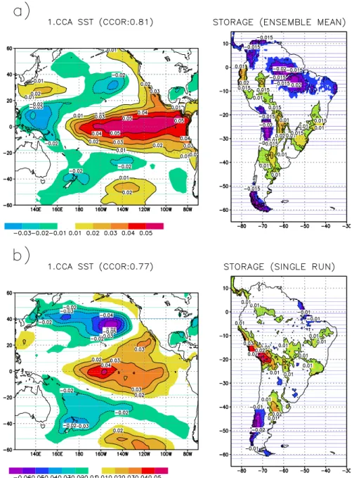
Fig. 4. 1.CCA of the pacific SST (60◦S–60◦N, 120◦E–70◦W) and the South American total water storage of the ensemble mean of 4simulations (a) and one single simulation (b). The right panel show the wavelet power spectrum of the amplitude of the canonical pattern, respectively.
The 1.EOF (Fig. 2) of the water storage of the ensem-ble mean of the ECHAM4-forced simulations explains more than a quarter (26, 2%) of the total variability. The pattern shows maximum variations in the Northern and Central parts of Brazil with maximum values in the Northeast. The coastal and west andean region of Peru and Northern Chile offers positive anomalies of the water storage as well, while most of the Southern parts of South America show negative varia-tions with the exception of the Paran´a river and Patagonia. This variability mainly represents interannual and decadal variations of the South American water storage, which is shown by the Wavelet Power spectrum of the corresponding
amplitude of the EOF (Fig. 2, right panel). It has a significant variability in the 1980’ies, starting with the El Ni˜no event of 1982/83, and also in the 1920’ies and 1930’ies with a pe-riod of approximately 5 years. But the spectrum shows also a permanent signal around periods of 10 to 15 years over the whole time-frame with a 5% significance at the end of the time series. This coexistence of interannual and decadal variations suggests an influence of the ENSO, but also, per-haps, of its decadal modulation, the Pacific Decadal Oscil-lation (PDO, Zhang et al. (1997)). This is confirmed by the work of Cobb et al. (2001) as well. They found a significant correlation between central tropical Pacific SST (corals) and
232 Stuck et al.: ENSO impact on South American hydro-climatology
Stuck et al.: ENSO impact on South American hydro-climatology 5
Fig. 4. 1.CCA of the pacific SST (60oS - 60oN, 120oE - 70oW)
and the South American total water storage of the ensemble mean of 4 simulations (a) and one single simulation (b). The right panel show the wavelet power spectrum of the amplitude of the canonical pattern, respectively.
lated with the water storage of Ecuador, Peru and Northern Chile. Additionally a series of time lagged correlations is constructed to demonstrate the evolution of the ENSO cor-related anomalies of the water storage after the peak phase of an ENSO event. Figure 6 presents the correlation and the regression of the water storage with the NINO3.4 index. The water storage reflects mainly the typical precipitation anomalies accompanied with an ENSO event. Significant positive correlations occur in the coastal areas of Ecuador and Northern Peru when the ENSO event peaks (lag 0) and negative correlations can be found in Southern Peru, the Altiplano, parts of the Atacama desert and North-West Ar-gentina. While those negative correlations enhance and last for at least 6 to 8 months, the positive anomalies in Ecuador and Northern Peru decreases slowly with time. Only in the central parts of Peru some weak but significant correlations develop or last until a time lag of 6 months. The Ecuadorian rainfall and as a result, the water storage is much higher cor-related to SST anomalies off the Pacific coast (NINO1+2), as it is highlighted by the difference of correlation of the water storage with the NINO1+2 and the NINO3.4 region (Fig. 7). The higher correlation with increased coefficients up to more than 0.2 is concentrated only on the coastal line. This
differ-Fig. 5. Wavelet power spectra of the amplitude of the canonical pattern (Fig. 4), respectively. Same labelling as Fig. 2
ence decreases with time until after 6 months the correlations with both indices are nearly the same. Otherwise, central parts of Peru are directly (lag 2&4) more affected by SST anomalies in the central tropical Pacific (NINO3.4), while the off coastal SST anomalies (NINO1+2) affect those areas later on (lag 8&10). In contrast, the negative correlations with the SST indices in Northern Chile and North-Western Argentina are higher with the NINO3.4 index for all time lags. In particular after 8 months the correlation is remark-ably larger, which means drier conditions in El Ni˜no years defined by NINO3.4. This different behaviour of the water storage in respect to the various ENSO indices demonstrates the complex response of the hydro-climate to Pacific SST variations. While for some regions like the coastal zone of Ecuador and Northern Peru the SST anomalies off the coast are more important than the central Pacific SST, where the typical ENSO-indices are estimated, most of the non-coastal areas are more affected by those central Pacific SST. These correlations patterns and time evolutions are also con-firmed by the CRU-forced WGHM simulation (not shown).
4 Conclusions
The South American hydro-climatology is analysed in re-spect to the El Ni˜no Southern Oscillation and its impact on the water storage. The variability is significantly influenced by the ENSO, in particular in the Amazon basin and at the
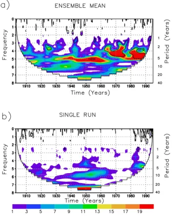
Fig. 5. Wavelet power spectra of the amplitude of the canonical pattern (Fig. 4), respectively. Same labelling as Fig. 2.
rainfall in North-Eastern Brazil with periods of 12–13 years. The 2.EOF (not shown) did not represent a typical ENSO response, either. Thus, the continental scale variability of South America is certainly not only influenced by the ENSO, but some typical regional coherencies are already be identi-fied by the 1.EOF.
The 1.EOF of the CRU-forced simulated water storage (Fig. 3) shows a very different pattern compared to the ECHAM-forced EOF. The pattern of the 1.EOF shows pre-dominantly a dipole structure of the anomalies of the water storage with positive values in the Northern part of South America, which peaks in the Amazon river with anomalies of 400 mm water equivalent, and negative anomalies in the Southern part. It explains similarly a quarter (24.3%) of the total variability of the simulated water storage, but there is no typical allocation in the time-frequency domain (Fig. 3, right panel). Only in 1982/83 a significant signal in the amplitude of the 1.EOF with a period of 2 years is coherent with the well-known El Ni˜no event. Such a phase relation between the ENSO and a 2-year signal in climate variates is also well known, but it originates from the stratospheric Quasi Bien-nial Oscillation (QBO, Gray et al. (1992)) or from the Tro-pospheric Biennial Oscillation (TBO, Meehl (1987)). Since those variations are focused either on the stratosphere or on the Western Pacific and Asia, it is improbable, that this 2-year signal of the South American hydro-climatology is linked to those TBO or QBO.
That difference between the EOF of the CRU-forced model run and the EOF of the ensemble mean of the ECHAM-forced runs is not surprising, since the signal-to-noise ratio is improved by the constitution of the ensemble mean and since the underlying time period of both simula-tions is different. But also the comparison with only one sin-gle run (not shown) shows few coincidencies with the CRU-forced EOF.
Thus, a simple principal component analysis is not able to detect the typical ENSO impact on the simulated South American water storage variations. Now, a canonical cor-relation analysis (CCA) shall provide the ENSO signal on the water storage variability of South America. There-fore we have used the Pacific SST (60◦S–60◦N, 120◦E– 70◦W) from the GISST dataset, which are used to force the ECHAM4 simulations, and the simulated grid cell data of the total water storage. This CCA maximises the linear relation-ship of two variates.
The analysis is applied to the ensemble mean of the simu-lated total water storage of the ECHAM-forced runs (4a) and to one single ECHAM-forced simulation alone (4b). The first canonical correlation patterns of the ensemble mean analy-sis yields a SST variability, which describes the typical SST anomaly of an El Ni˜no event. The maximum canonical cor-related (0.81) water storage variation pattern of the ensemble mean shows most of the expected anomalies as far as they are expectedly. Due to the well known strong increased pre-cipitation in the coastal areas of Ecuador and Peru the water storage offers positive anomalies in these areas when the SST anomaly peaks in boreal winter. Likewise the pattern consists of positive anomalies in central Chile, Southern Brazil and Northern Argentina. Decreased water storage can be found in Southern Peru and Northern Chile and in the Amzon basin in the North of Brazil as well. Most of these areas are also de-tected by the ANOVA (Fig. 1) by significantly explained vari-ance of the water storage in ENSO years. The spectral be-haviour of the amplitude of the SST and the water storage is presented by the wavelet power spectrum (Fig. 5a) and shows the typical variations of the ENSO. The spectrum looks abso-lutely the same as the spectrum of a SST-based ENSO index series like NINO3 or NINO3.4 (e.g. Torrence and Compo (1998), their Fig. 1b), which confirms the assumption, that these CCA patterns represent the typical ENSO variability.
The same analysis, with only one realisation of the ECHAM-forced model run, shows a similar pattern of SST variations for the 1.CCA mode (Fig. 4b). But anyhow those variations represent a complete different mode of variabil-ity. For example, the pattern shows no SST anomalies off the South American Pacific coast, where usually the strongest SST anomalies of an ENSO event occur. The amplitude of this CCA pattern gives no hint for a linkage with the ENSO. It consists of a nearly decadal signal between 1940 and 1960 and some weak interannual signals in the same period and in the 1980ies (Fig. 5b). But all of these signals are not significant at the 5% level. Accordingly, the correspond-ing total water storage variations did not display any typi-cal ENSO-caused variation. The same holds for the CCA
Stuck et al.: ENSO impact on South American hydro-climatology 233
6
Stuck et al.: ENSO impact on South American hydro-climatology
Fig. 6. Correlation and regression of the NINO3.4 index with the
total water storage of the ensemble mean of 4 simulations
(1961-1994) for the region of Ecuador, Peru and Northern Chile with a
time lag of 0, 2, 4, 6, 8 and 10 month (positive lag means NINO3.4
leads the water storage). Shaded information represent correlation
(contour intervall: 0.1), contour lines represent regression (contour
intervall: 5 mm water equvalent).
coastal areas of Ecuador and Peru. In some of these areas the
simulated water storage variability is explained up to more
than 70% by tropical Pacific SST anomalies. These high
values of explained variance lead to a general seasonal
pre-dictability of the water storage variations. The model results
of the different forcing data, one from an observational basis,
represented by the CRU data set, and one from the model
out-Fig. 7. Difference of correlation and regression of the NINO1+2
index with the total water storage of the ensemble mean of 4
simu-lations (1961-1994) and the correlation and regression of NINO3.4
(Fig. 6). Contour intervall of shadings (correlation): 0.05, contour
lines (regression): 5 mm water equivalent.
put of a climate simulation, the ECHAM4-T42 GCM, which
is forced with observed SST values, show a very diverse
re-sponse to the ENSO. Only the regional univariate correlation
analyses reveal very similar results for both simulations in
Ecuador, Peru and Chile. The advantage of the constitution
of an ensemble mean of the ECHAM-forced simulations is
reflected in the result of the maximum canonical correlation
patterns of the Pacific SST and the South American water
storage anomalies. This coherent mode represents the
typ-Fig. 6. Correlation and regression of the NINO3.4 index with the total water storage of the ensemble mean of 4 simulations (1961–1994) forthe region of Ecuador, Peru and Northern Chile with a time lag of 0, 2, 4, 6, 8 and 10 month (positive lag means NINO3.4 leads the water storage). Shaded information represent correlation (contour intervall: 0.1), contour lines represent regression (contour intervall: 5 mm water equvalent).
234 Stuck et al.: ENSO impact on South American hydro-climatology
6
Stuck et al.: ENSO impact on South American hydro-climatology
Fig. 6. Correlation and regression of the NINO3.4 index with the
total water storage of the ensemble mean of 4 simulations
(1961-1994) for the region of Ecuador, Peru and Northern Chile with a
time lag of 0, 2, 4, 6, 8 and 10 month (positive lag means NINO3.4
leads the water storage). Shaded information represent correlation
(contour intervall: 0.1), contour lines represent regression (contour
intervall: 5 mm water equvalent).
coastal areas of Ecuador and Peru. In some of these areas the
simulated water storage variability is explained up to more
than 70% by tropical Pacific SST anomalies. These high
values of explained variance lead to a general seasonal
pre-dictability of the water storage variations. The model results
of the different forcing data, one from an observational basis,
represented by the CRU data set, and one from the model
out-Fig. 7. Difference of correlation and regression of the NINO1+2
index with the total water storage of the ensemble mean of 4
simu-lations (1961-1994) and the correlation and regression of NINO3.4
(Fig. 6). Contour intervall of shadings (correlation): 0.05, contour
lines (regression): 5 mm water equivalent.
put of a climate simulation, the ECHAM4-T42 GCM, which
is forced with observed SST values, show a very diverse
re-sponse to the ENSO. Only the regional univariate correlation
analyses reveal very similar results for both simulations in
Ecuador, Peru and Chile. The advantage of the constitution
of an ensemble mean of the ECHAM-forced simulations is
reflected in the result of the maximum canonical correlation
patterns of the Pacific SST and the South American water
storage anomalies. This coherent mode represents the
typ-Fig. 7. Difference of correlation and regression of the NINO1+2 index with the total water storage of the ensemble mean of 4 simula-tions (1961–1994) and the correlation and regression of NINO3.4 (Fig. 6). Contour intervall of shadings (correlation): 0.05, contour lines (regression): 5 mm water equivalent.
Stuck et al.: ENSO impact on South American hydro-climatology 235 analysis using the CRU-forced simulated water storage (not
shown). The maximum canonical correlation did not bring out the typical ENSO variations. This emphasizes clearly the advantage of the constitution of the ensemble mean. With the improvement of the signal-to-noise ratio the signal is de-tectable, but on the other hand, the signal is that weak, that it isn’t detectable in one realisation of the South American hydro-climatology alone. This is attributed to the complex space-time structure or rather the non-linear behaviour of the precipitation and the water storage as well.
These correlations patterns and time evolutions are also confirmed by the CRU-forced WGHM simulation (not shown).
4 Conclusions
The South American hydro-climatology is analysed in re-spect to the El Ni˜no Southern Oscillation and its impact on the water storage. The variability is significantly influenced by the ENSO, in particular in the Amazon basin and at the coastal areas of Ecuador and Peru. In some of these areas the simulated water storage variability is explained up to more than 70% by tropical Pacific SST anomalies. These high values of explained variance lead to a general seasonal pre-dictability of the water storage variations.
The model results of the different forcing data, one from an observational basis, represented by the CRU data set, and one from the model output of a climate simulation, the ECHAM4-T42 GCM, which is forced with observed SST values, show a very diverse response to the ENSO. Only the regional univariate correlation analyses reveal very sim-ilar results for both simulations in Ecuador, Peru and Chile. The advantage of the constitution of an ensemble mean of the ECHAM-forced simulations is reflected in the result of the maximum canonical correlation patterns of the Pacific SST and the South American water storage anomalies. This coherent mode represents the typical variations of the wa-ter storage affected by the ENSO. The SST patwa-tern shows the typical Pacific SST anomaly during the peak phase of an El Ni˜no event and the water storage anomaly pattern reflects those variations, which are expected due to some well-known rainfall anomalies. In contrast to the SST pattern, which could be validated by observed data (e.g. SST anomaly in 1982/83), the water storage could not be validated since no observational data of the water storage exist, in particular on the continental scale. Since water storage variations can now be resolved for large areas by observing the gravity field, such validation could be possible in future given the mag-nitude of the continental water storage signal that is caused by strong ENSO events.
The regional correlation analysis pointed out, that a com-mon definition of ENSO did not exist. Some areas, in par-ticular coastal areas of Ecuador and Northern Peru are more sensitive to the SST anomalies off the coast of Ecuador and Peru, defined by the NINO1+2 index, while areas more
dis-tant to the tropical Pacific coast are more affected by the cen-tral tropical SST anomalies, defined by the NINO3.4 index. Acknowledgements. The authors thank J. Alcamo (Center for Environmental Systems Research, University of Kassel, Germany) and P. D¨oll (Dept. Physical Geography, University of Frankfurt, Germany) for providing the WGHM code.
Edited by: P. Fabian and J. L. Santos
Reviewed by: M. Richter and another anonymous referee
References
Aceituno, P.: On the functioning of the Southern Oscillation in the South American sector, part I: surface climate, Mon. Wea. Rev., 116, 505–524, 1988.
Amarasekera, K. N., Lee, R. F., Williams, E. R., and Eltahir, E. A. B.: ENSO and the natural variability in the flow of tropical rivers, J. Hydrol., 200, 24–39, 1997.
Andersen, O. B. and Hinderer, J.: Global inter-annual gravity changes from GRACE: Early results, Geophys. Res. Lett., 32, L01402, doi:01410.01029/2004GL020948, 2005.
Bretherton, C. S., Smith, C., and Wallace, J. M.: An Intercompari-son of Methods for Finding Coupled Patterns in Climate Data, J. Climate, 5, 541–560, 1992.
Cobb, K. M., Charles, C. D., and Hunter, D. E.: A central tropical Pacific coral demonstrates Pacific, Indian, and Atlantic decadal climate connections, Geophys. Res. Lett., 11, 2209–2212, 2001. D¨oll, P., Kaspar, F., and Lehner, B.: A global hydrological model for deriving water availability indicators: model tuning and vali-dation, J. Hydrol., 270, 105–134, 2003.
Enfield, D.: Relationship of inter-American rainfall to tropical At-lantic and Pacific SST variability, Geophys. Res. Lett., 23, 3305– 3308, 1996.
Fu, R., Dickinson, R. E., Chen, M., and Wang, H.: How do Tropical Sea Surface Temperatures Influence the Seasonal Distribution of Precipitation in the Equatorial Amazon?, J. Climate, 14, 4003– 4026, 2001.
Glynn, P. W.: Global ecological consequences of the 1982–83 El Ni˜no Southern Oscillation, Elsevier, New York, 1990.
Gray, W. M., Scheaffer, J. D., and Knaff, J. A.: Influence of the stratospheric QBO on the ENSO variability, J. Meteor. Soc. Japan, 70, 975–995, 1992.
Kutzbach, J.: Empirical Eigenvectors of Sea-Level Pressure, Sur-face Temperature, and Precipitation Complexes over North America, J. Appl. Meteor., 6, 791–802, 1967.
Meehl, G. A.: The Annual Cycle and Interannual Variability in the Tropical Pacific and Indian Ocean Region, Mon. Wea. Rev., 115, 27–50, 1987.
New, M. G., Hulme, M., and Jones, P. D.: Representing 20th cen-tury space-time climate variability. II: development of 1901–96 monthly grids of terrestrial surface climate, J. Climate, 13, 2217– 2238, 2000.
Ngo-Duc, T., Laval, K., Polcher, J., Lombard, A., and Cazenave, A.: Effects of land water storage on global mean sea level over the past half century, Geophys. Res. Lett., 32, L09704, doi:09710.01029/2005GL022719, 2005.
Preisendorfer, R. W.: Principal component analysis in meteorology and oceanography, edited by: Mobley, C. D., Elsevier Science Publishers, Developments in Atmospheric Science, 17, 1988.
236 Stuck et al.: ENSO impact on South American hydro-climatology
Ramillien, G., Frappart, F., Cazenave, A., and G¨untner, A.: Time variation of land water storage from an inversion of 2 years of GRACE geoids, Earth and Planetary Science Letters, in print, 2005.
Rayner, N. A., Horton, E. B., Parker, D. E., et al.: Version 2.2 of the global sea-ice and sea surface temperature data set, 1903–1994, CRTN, 74, Hadley Centre, Bracknell, UK, 1996.
Richey, J. E., Nobre, C., and Deser, C.: Amazon river discharge and climate variability: 1903–1985, Science, 246, 101–103, 1989. Roeckner, E., Arpe, K., Bengtsson, L., et al.: The atmospheric
gen-eral circulation model ECHAM-4: Model description and simu-lation of present day climate, MPI-Report, 218, Max Plank Insti-tut f¨ur Meteorologie, Hamburg, 1996.
Ropelewski, C. F. and Halpert, M. S.: Global and regional scale precipitation patterns associated with the El Ni˜no/Southern Os-cillation, Mon. Wea. Rev., 115, 1606–1612, 1987.
Rowell, D. P., Folland, C. K., Maskell, K., and Ward, M. N.: Vari-ability of Summer Rainfall over Tropical North Africa (1906– 92): Observations and Modelling, Q. J. R. Meterol., 121, 669– 704, 1995.
Schmidt, R., Schwintzer, P., Flechtner, F., Reigber, C., G¨untner, A., D¨oll, P., Ramillien, G., Cazenave, A., Petrovic, S., Jochmann, H., and W¨unsch, J.: GRACE observations of changes in continental water storage, Global and Planetary Change, in print, 2005.
Tapley, B. D., Bettadpur, S. V., Watkins, M., and Reigber, C.: The gravity recovery and climate experiment: Mission overview and early results, Geophys. Res. Lett., 31, L09607, doi:09610.01029/2004GL019920. 2004a.
Tapley, B. D., Bettadpur, S. V., Ries, J. C., Thompson, P. F., and Watkins, M.: GRACE measurements of mass variability in the Earth system, Science, 305, 503–505, 2004b.
Torrence, C. and Compo, G. P.: A Practical Guide to Wavelet anal-ysis, Bull. Amer. Meteor. Soc., 79, 61–78, 1998.
von Storch, H. and Zwiers, F. W.: Statistical Analysis in Cli-mate Research, Cambridge University Press, Cambridge, 484 pp., 1999.
Vuille, M.: Atmospheric circulation anomalies over the Bolivian Altiplano during dry and wet periods and extreme phases of the Southern Oscillation, Int. J. Climatol., 19, 1579–1600, 1999. Wahr, J., Swenson, S., Zlotnicki, V., and Velicogna, I.:
Time-variable gravity from GRACE: First results, Geophys. Res. Lett., 31, L11501, doi:11510.11029/2004GL019779, 2004.
Waylen, P. and Poveda, G.: El Ni˜no-Southern Oscillation and as-pects of western South American hydro-climatology, Hydrol. Process., 16, 1247–1260, 2002.
Zhang, Y., Wallace, J. M., and Battisti, D. S.: ENSO-like inter-decadal variability: 1900–93, J. Climate, 10, 1004–1020, 1997.