Design and development of a novel liquid desiccant air-conditioning system

Design and Development of a Novel Liquid Desiccant

Air-Conditioning System

by

Ross A. Bonner

Submitted to the Department of Mechanical Engineering

in partial fulfillment of the requirements for the degree of

Master of Science in Mechanical Engineering

at the

MASSACHUSETTS INSTITUTE OF TECHNOLOGY

September 2020

c

○ Massachusetts Institute of Technology 2020. All rights reserved.

Author . . . .

Department of Mechanical Engineering

September 16, 2020

Certified by . . . .

Douglas Hart

Professor

Thesis Supervisor

Accepted by . . . .

Nicolas Hadjiconstantinou

Chairman, Department Committee on Graduate Theses

Design and Development of a Novel Liquid Desiccant

Air-Conditioning System

by

Ross A. Bonner

Submitted to the Department of Mechanical Engineering on September 16, 2020, in partial fulfillment of the

requirements for the degree of

Master of Science in Mechanical Engineering

Abstract

The Direct Evaporative Closed Air Loop (DECAL) system is a novel high efficiency liquid desiccant air-conditioning (LDAC) system which runs primarily on thermal energy rather than electricity. It is designed for residential cooling in hot and humid climates where demand is growing rapidly and incumbent direct-expansion system performance is poor. Unlike other LDAC systems, DECAL is modular. This allows the indoor hardware to remain small and non-intrusive, and offers increased flexibility to install the system in existing building stock without costly changes to the structure. This work lays out the basic operating cycle of the DECAL system and shows its thermodynamic merits in terms of ideal system performance against other LDAC systems. Design studies show DECAL offers improved thermal efficiency, especially in humid climates. The ideal thermal coefficient of performance (COPth) is 1.24 at

the design point ambient condition of 35C, 60% RH. A mathematical model is built to better characterize performance and optimize the system design. With transport inefficiencies included, the optimal system electrical and thermal COP (COPe and

COPth) are 46.3 and 0.759 respectively for a LiCl system at the design point. These

results show the DECAL system could reduce electrical consumption by over 85% from present day best-in-class systems using low-grade thermal energy.

A benchtop scaled test of the closed air loop is constructed to validate the model. Experimental test results agree well with the model predictions for evaporative cooling effectiveness and sensible heat exchange, as well as pressure drop. The drying effect of the LAMEE is lower than anticipated. This is likely due to crystallization of liquid desiccant in the pores of the membrane, resulting in a high vapor diffusion resistance. Adjusting for this effect, full system test measurements match the system model well. The benchtop rig testing verified that the closed air loop is capable of generating a sensible cooling effect, but further testing is required to demonstrate modelled figures of merit are achievable.

Thesis Supervisor: Douglas Hart Title: Professor

Acknowledgments

This work sits atop a mountain of support, patience, and passion from an outstanding network of people. I owe each of you an enormous debt of gratitude and hope I’m able to pay forward your generosity and good will.

Julie - there are no words to express how grateful I am for everything you’ve done to make this possible. I find myself beginning to write one of those "gee, thanks for putting up with me!" aww shucks style thank you notes but that doesn’t begin to capture it. You really sacrificed for this, and in the end this is as much your accomplishment as it is mine. I hope you feel that. I know long nights for me are long nights for you, and my focus on this has stolen a lot of moments we could have shared. Going forward I’m going to make time to live in the moment and keep reminding you that every little thing is gonna be alright.

Mom - thank you for showing me through your example the importance of love, patience, and selflessness in service of others. You would be surprised how often your voice pops in my head to remind me not to "cut the head off" when I’m at risk of messing up a good thing because it isn’t quite perfect.

Dad - you taught me that great things come through hard work and just a pinch of stubbornness. Because of you I know the value of keeping myself above reproach and making sure the job is done right before putting my name on it.

Doug and Peter - thank you for introducing me to the challenge of low carbon cooling back in 2.013, and for sparking a real passion in me that has pushed me to expand my horizons to make the world a better place.

To GE aviation and all my friends at GE - thank you for sponsoring my tuition at MIT and nurturing my growth as an engineer through the Edison program and beyond. Special thanks to Tyler Hooper, Phil Weed, Paul Patoulidis, Rob Brown, Alan Grissino, and Don Desander who mentored me throughout my time at GE.

Alex - thanks for being there for me throughout ASP so I wasn’t going it alone. You gave me a place to park near Kendall, a friendly face to de-stress with at the Muddy after a long week, and most importantly you always made me look good by

showing up just slightly later than I did!

Leslie Regan - thanks for going out of your way (several times) to go to bat for me when I fell short on administrative tasks and deadlines 101. Having such a staunch advocate in the department always made MIT feel like home.

Sorin and Matt - thanks for seeing potential in me and giving me a platform to take the climate-change-fighting spirit from my thesis work and apply it in the startup world. I can’t wait to help make great things happen with Transaera.

Contents

1 Introduction 15

1.0.1 Climate Change . . . 15

1.1 Growing Demand for Space Cooling . . . 16

1.1.1 Climate Factors . . . 17

1.1.2 Economic Factors . . . 18

1.1.3 Demographic Factors . . . 19

1.1.4 Implications for Energy Demand . . . 20

1.2 The State of the Art . . . 20

1.2.1 Vapor Compression . . . 20

1.2.2 Ground Source Heat Pumps . . . 27

1.2.3 Evaporative Cooling . . . 29

1.2.4 Desiccant Dehumidification . . . 30

1.2.5 LAMEEs . . . 33

1.2.6 Liquid Desiccant Cooling . . . 33

2 System Design 37 2.1 Figures of Merit and Design Constraints . . . 37

2.1.1 Physical Envelope . . . 39

2.1.2 Thermal Coefficient of Performance . . . 39

2.1.3 Electrical Coefficient of Performance . . . 40

2.1.4 Cooling Unit Airflow . . . 41

2.2 System Overview . . . 42

2.4 Air Process Loop . . . 47

2.5 LD Cooling Loop . . . 48

2.6 LD Process Loop . . . 49

2.7 Ideal Cycle Limits and Benchmarking . . . 50

3 Mathematical Model 55 3.1 Solver Routine . . . 56

3.2 Sensible Heat Exchanger . . . 59

3.2.1 Outlet State Calculations . . . 59

3.2.2 Physical Envelope . . . 60

3.2.3 Pressure Drop and Power Draw . . . 63

3.3 Liquid-Air Membrane Energy Exchanger . . . 65

3.3.1 Outlet State Calculations . . . 65

3.3.2 Physical Envelope . . . 67

3.3.3 Power Draw . . . 67

3.4 Direct Evaporative Cooler . . . 68

3.4.1 Outlet State Calculations . . . 68

3.4.2 Physical Envelope . . . 69

3.4.3 Power Draw . . . 69

3.5 Ancillary Subroutines . . . 70

3.5.1 Air State Calculations . . . 70

3.5.2 Liquid Desiccant State Calculations . . . 72

3.6 Model Results . . . 73

3.6.1 Exchanger Efficiency Sweep . . . 73

3.6.2 Design Space Exploration . . . 75

4 Experimental Validation 79 4.1 Covid19 . . . 79

4.2 Test Rig Design . . . 80

4.2.1 DEC Module Design . . . 81

4.2.3 LAMEE Module Design . . . 85

4.2.4 Instrumentation . . . 87

4.3 Testing . . . 89

4.3.1 DEC Effectiveness Testing . . . 89

4.3.2 SHX Effectiveness Testing . . . 90

4.3.3 Full System Performance Testing . . . 91

5 Conclusions 95 5.1 Lessons Learned . . . 96

5.2 Future Work . . . 97

A Tables 99

List of Figures

1-1 Cumulative CO2 Emissions vs Surface Temperature Change [25] . . . 17

1-2 Projected global air conditioner stock 1990-2050 (millions) . . . 18

1-3 Per-capita income vs rate of AC ownership [3] . . . 19

1-4 Heat Pump in Cooling Configuration . . . 22

1-5 Cooling Load Conditions . . . 24

1-6 Performance of US Energy Star Certified Systems vs Cooling Capacity [41] . . . 25

1-7 Ground Source Heat Pump in Cooling Configuration . . . 28

1-8 Flow and process diagrams for DEC, IEC, and dew point cooling . . 30

1-9 Solid and Liquid Desiccant Dehumidification Systems . . . 32

1-10 DEVap Cooling Core . . . 35

2-1 Energy Star Split Systems Specific Volume . . . 40

2-2 DECAL Simplified System Diagram . . . 42

2-3 Full System Schematic . . . 45

2-4 DECAL Staged Evaporative Cooling . . . 46

2-5 Air Process Loop Cycle and Diagram . . . 48

2-6 LD Cooling Loop Cycle and Diagram . . . 49

2-7 LD Process Loop Cycle and Diagram . . . 50

2-8 System Diagrams for Ideal Limits Studies . . . 52

2-9 Ideal Limits Thermal COP . . . 53

3-1 Mathematical Model Architecture . . . 56

3-3 Process SHX Air Side Channel Geometry . . . 61

3-4 Liquid Desiccant and Water Vapor Equilibrium - CaCl2 and LiCl . . 73

3-5 System Figures of Merit vs Exchanger Efficiency . . . 74

3-6 Design Exploration Results . . . 77

4-1 Benchtop Test Block Diagram . . . 81

4-2 Benchtop Test Rig . . . 82

4-3 Direct Evaporative Cooler Module . . . 83

4-4 DEC Module Subassembly . . . 84

4-5 Direct Evaporative Cooler Module . . . 85

4-6 Sensible Heat Exchanger Module . . . 86

4-7 LAMEE Layers and Flow Pattern . . . 87

4-8 System Instrumentation Layout . . . 88

4-9 Left: Instrumented U-Duct Assembly Right: Split Ducts As-Printed . 89 4-10 DEC Effectiveness vs Face Velocity . . . 90

4-11 SHX Effectiveness vs Face Velocity . . . 91

4-12 Full System Test Results . . . 93 B-1 Liquid Desiccant State Calculations - CaCl2 Solubility Limit Validation 101

B-2 Liquid Desiccant State Calculations - LiCl Solubility Limit Validation 102 B-3 Liquid Desiccant State Calculations - CaCl2 Vapor Pressure Validation 102

List of Tables

1.1 Typical SHR range for US climate zones . . . 23

1.2 Global warming potential of common refrigerants . . . 27

2.1 Sizing Conditions Used In This Study . . . 39

2.2 Figure of Merit Targets . . . 42

3.1 Range of Efficiencies Used in Design Exploration Study . . . 75

3.2 Design Exploration Study Requirements Summary . . . 76

3.3 Optimized Design Performance at Design Point . . . 76

Chapter 1

Introduction

This work details the design and development of an energy-efficient air conditioning system which runs primarily on low-grade heat. The aim of this research is to fill the growing need for human cooling without further contributing to climate change. To achieve this goal, a step-change improvement in efficiency is needed in the near future. This chapter establishes the urgent need for high-efficiency air conditioning, reviews some of the pertinent principles, and summarizes the state of the art and recent advances in the literature.

1.0.1

Climate Change

Climate change presents a challenge of unprecedented scale, and the window to avoid the most severe consequences is extremely narrow. The actions we take now could make the difference between 1.5C warming and 2C warming, and the difference be-tween these two scenarios is dramatic. In broad terms, to achieve 1.5C warming, we must reduce net CO2 emissions by 45% from 2010 levels by 2030, and achieve net zero by 2050. 2C pathways correspond to 25% reduction by 2030 and net zero in 2070. This reduction requires annual investment in low-carbon technology and energy efficiency to increase sixfold by 2050 [25].

The International Energy Agency (IEA) lays out two scenarios to illustrate the changes possible through intelligent energy policy and technology. The "Current

Poli-cies" scenario which assumes business as usual, and the "Sustainable Development" scenario which avoids the worst consequences of global warming, and supports the United Nations Sustainable Development Goals (SDGs), including universal access to modern energy by 2030 (SDG 7). Dramatic increases in energy efficiency are at the heart of the Sustainable Development scenario, and our current trend is not improv-ing fast enough. [4] The IPCC states mitigation ambitions in the Paris Agreement are not sufficient to limit global warming to 1.5C. Even if scaled up significantly after 2030, global emissions must begin to decline well before 2030. [25] The IEA Sustain-able Development scenario reaches carbon neutral around 2070, but does not meet 1.5C without use of carbon capture and sequestration (CCS). [4]

Global mean surface temperature (GSMT) has already risen around 1C above pre-industrial levels, and is increasing at a rate of 0.2C per decade. Depending on the method of approximation, the remaining budget to achieve a 50% probability of remaining under 1.5C warming is between 580 and 770 GtCO2, with the difference

primarily being the treatment of Earth system feedbacks such as the thawing of permafrost. [25]

Our collective leverage to bend the energy curve down is strongest now and only gets weaker over time, so the time is now to reduce our energy demand through innovation.

1.1

Growing Demand for Space Cooling

According to the IEA, the increasing demand for space cooling is "one of the most critical blind spots in today’s energy debate". Use of air conditioners and electric fans to cool an occupied space (collectively referred to as space cooling) accounts for around 20% of total electricity used in buildings worldwide. Energy use for space cooling has more than tripled between 1990 and 2016, with unit sales quadrupling up to 135 million units in the same time frame. Space cooling is the fastest growing end use of energy in buildings. [3]

Figure 1-1: Cumulative CO2 Emissions vs Surface Temperature Change [25]

1.1.1

Climate Factors

As the earth warms, naturally the demand for cooling increases. According to the IPCC, an increase of 1.5C corresponds to an even more pronounced increase in ex-treme hot days. At 1.5C GSMT warming, the temperature of exex-treme hot days (heat waves) increases 3C. This figure jumps to 4C at 2C GSMT warming. Additionally, temperature increases are more extreme over land, and may be accompanies by other changes in weather, increasing precipitation in some regions and drought in others. [25]

Climate driven demand for cooling is correlated to the number of cooling degree days (CDDs), which capture the total time and extent to which the ambient tem-perature exceeds a reference condition. In many populous regions such as Western Europe, household space cooling is uncommon (only 3% in the UK and Germany and 5% in France). However, as climate change slowly turns up our collective global

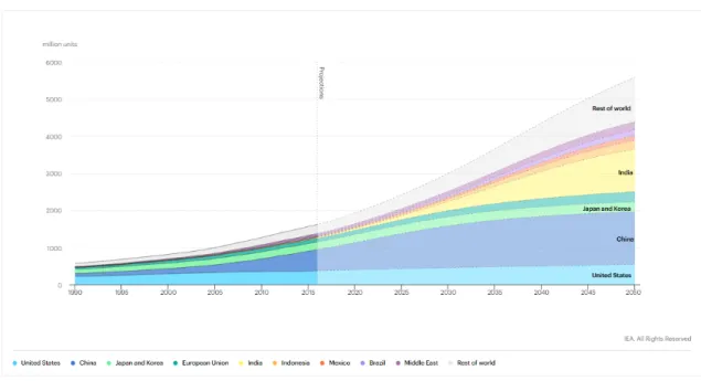
Figure 1-2: Projected global air conditioner stock 1990-2050 (millions)

thermostat, heat waves in these areas increase in frequency. These weather events serve as pain points which drive consumers to invest in AC, leading to a permanent increase in cooling energy demand, even if following Summer temperatures are lower. The regions with the greatest projected increase in CDDs by 2050 also have the fastest growth rates in population and income. The confluence of these three factors explains the striking increases in demand discussed in this chapter. Climate change is perhaps the most intuitive contributing factor for increasing cooling demand, but it is not the only important driver. [3]

1.1.2

Economic Factors

While climate sets the latent demand for space cooling, economic factors determine to what extent consumers are able to satisfy that demand. While the climates of India and Singapore are similar in terms of CDDs, it is estimated that in Singapore (2018 per-capita GDP = $64,581), 99% of apartments have AC, while in India (2018 per-capita GDP = $2010), only 4% of households have AC. [7][23] While the current market penetration of AC in India is quite low, it is rising rapidly there and in the many other developing countries with hot climates. The clear relationship between

prosperity, climate, and household AC ownership is shown in Figure 1-3. Each data point represents a country, colored by CDD. The high density of red points at the left of the chart indicates the large populations in need of AC but restricted by poverty. Most homes in these hot and poor countries have not yet purchased their first AC, but by 2050 about two-thirds of households worldwide will be AC-equipped. [3]

Figure 1-3: Per-capita income vs rate of AC ownership [3]

1.1.3

Demographic Factors

Ignoring all other factors, the world’s increasing population alone will drive an increase in cooling demand (and energy demand as a whole). The UN projects an increase in global population from 7.8B in 2020 to 9.7B in 2050. The more complete picture shows several additional factors which bias toward a growing demand for AC. Population growth over in the next 30 years is highest in the hottest parts of the world, largely sub-Saharan Africa. [35] Urbanization also contributes to rising cooling demand. An increasingly urban population means more people working indoors, driving additional demand. Furthermore, the heat island effect drives up ambient temperatures in cities due to a combination of factors, including a significant effect from heat rejection of space cooling systems themselves. The aging population also drives a need for cooling, as older people are generally less heat-tolerant than young. In many cases AC for the elderly is a matter of public health. Hospitalization and mortality rates for the elderly are both known to spike in the wake of heat waves. In the next 30 years, the

percentage of global population over age 60 is projected to increase from 13% to 25% in all regions except Africa. [3]

1.1.4

Implications for Energy Demand

Cooling energy demands put significant strain on the energy grid, especially at peak times. In the Middle East and some parts of the United States, cooling loads represent more than 70% of peak residential electricity demand on the hottest days. [3]

1.2

The State of the Art

1.2.1

Vapor Compression

The vast majority of today’s space cooling units are vapor compression systems (VCS) [3]. VCS transfer heat against the natural gradient from a low temperature source to a high temperature sink. The performance of VCS is expressed by the coefficient of performance (COP), see eqn. 1.1.

𝐶𝑂𝑃𝑅= 𝐶𝑜𝑜𝑙𝑖𝑛𝑔 𝑃 𝑜𝑤𝑒𝑟 𝑊 𝑜𝑟𝑘 𝐼𝑛𝑝𝑢𝑡 = 𝑄𝑐𝑜𝑜𝑙 𝑊𝑖𝑛 (1.1) In its most ideal form, the vapor compression cycle is a reversed Carnot cycle. At the limit, the performance of such a system is given by the Carnot COP, see eqn. 1.2.

𝐶𝑂𝑃𝐶𝑎𝑟𝑛𝑜𝑡 =

𝑇𝑐𝑜𝑙𝑑

𝑇ℎ𝑜𝑡− 𝑇𝑐𝑜𝑙𝑑

(1.2) Where 𝑇𝑐𝑜𝑙𝑑 is the temperature of the refrigerant in the evaporator and 𝑇ℎ𝑜𝑡 is

the temperature of the refrigerant in the condenser. In industry, two additional terms, energy efficiency ratio (EER) and seasonal energy efficiency ratio (SEER) are commonly used to describe air conditioning performance. EER describes the same metric as COP but is specific to cooling systems (whereas COP can also describe a heat pump in heating mode). EER also implies a specific test condition, which varies by region. In the US EER is tested at an ambient condition of 35C, 50% RH.

Furthermore, in the US, EER by convention uses British thermal units (BTU) for cooling power provided and Watt-hrs (Wh) for work input, requiring a conversion from EER to COP, see eqn. 1.3.

𝐸𝐸𝑅𝑈 𝑆 =

𝐶𝑜𝑜𝑙𝑖𝑛𝑔 𝑃 𝑜𝑤𝑒𝑟 (𝐵𝑇 𝑈 )

𝑊 𝑜𝑟𝑘 𝐼𝑛𝑝𝑢𝑡 (𝑊 ℎ) = 3.412 𝐶𝑂𝑃 (1.3) SEER gives a more representative estimate of cooling performance over a typical cooling season. SEER is assigned by conducting a series of tests at varying outdoor conditions and calculating a weighted average which represents the cooling season for a particular region. This is useful for consumers as it gives a more accurate performance estimate when purchasing a system. However, since testing standards vary widely by climate, consistent benchmarking is difficult. In this work all benchmark comparisons are made with COP - EER and SEER are only referenced for comparisons between incumbent systems. [3]

The actual refrigeration cycle differs from the reverse Carnot cycle since the tur-bine is replaced by a throttling valve or capillary tube for practical reasons. This cycle is commonly referred to as direct expansion (DX) refrigeration. The ideal DX cycle consists of 4 processes. [13]

∙ Isentropic compression in compressor

∙ Constant pressure heat rejection in condenser ∙ Constant enthalpy throttling in throttling valve ∙ Constant pressure heat addition in evaporator

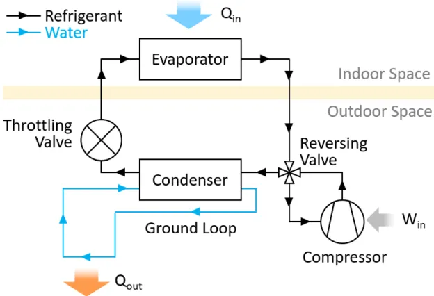
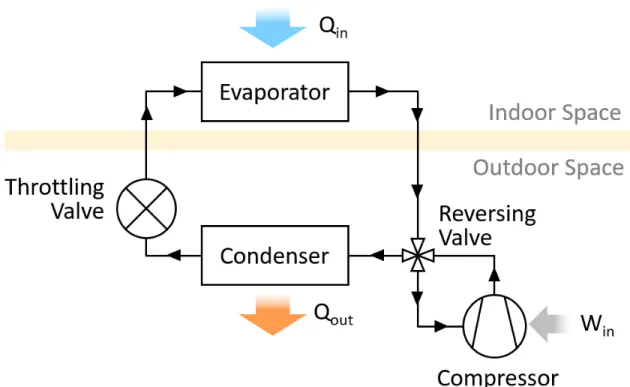
In many mild climates where cooling is needed in summer months and heating is needed in winter months, it is advantageous to run the system in reverse to provide heating. This is accomplished with minimal change to the hardware by including a reversing valve before the compressor. Systems equipped with this function are called heat pumps. Figure 1-4 shows the typical arrangement for a heat pump system operating in cooling mode.

Figure 1-4: Heat Pump in Cooling Configuration

The denominator term in eqn. 1.2 is the temperature difference between the condensing temperature and the evaporating temperature. The performance of the system can be improved by reducing this difference - i.e. lowering condenser tem-perature or raising evaporator temtem-perature. In order to transfer heat to the ambient environment, the condenser temperature must be above ambient. Similarly, the evap-orator temperature must be lower than the indoor space being cooled. The magnitude of this difference is dependent on the effectiveness of heat exchange between the air and refrigerant, so system efficiency may be improved by increasing the size of the condenser or evaporator. This also implies that for a given indoor temperature, when the ambient condition is hotter performance will be lower. To maintain a comfort-able condition in the cooled space, both the temperature and humidity of the space must be maintained to certain levels. An indoor condition of 27C and 60% relative humidity (RH) is around the upper limit of human thermal comfort and is used in this work as the standard cooled space condition.

Climate SHR Range

1A-3A. Hot/Humid (e.g. Houston) 0.0-0.9

4A-5A. Hot/Humid/Cold (e.g. Chicago) 0.0-1.0

2B. Hot/Monsoon (e.g. Phoenix) 0.7-1.0

3B-5B. Hot/Dry (e.g. Las Vegas) 0.8-1.0

4C. Marine (e.g. San Francisco) 0.5-1.0

Table 1.1: Typical SHR range for US climate zones

raise the temperature of the indoor space by heat addition, they come from solar irradiance and heat transfer from ambient air (envelope loads), and heat from oc-cupants, lighting, and electronics (internal loads). Latent loads raise the humidity of the indoor space, and come from air changes with the ambient space (if outdoor humidity is high), occupant respiration, cooking, and evaporation from any indoor free water surface. The total load on the building is the sum of all sensible and latent loads. The sensible heat ratio (SHR) is the ratio of sensible load to total load, and varies from 0 (all latent load) to 1 (all sensible load). Table 1.1 shows typical ranges for SHR in several US climates per ASHRAE zone conventions. [28]

Figure 1-5 shows cooling loads and how they are met with present day DX systems. Figure A shows sensible heat ratios from 1.0 - 0.4 from a room condition of 27C and 60% RH. As the fraction of latent load increases, SHR decreases and the load line becomes steeper. Figure B shows the components of latent load and sensible load. To maintain a consistent indoor condition, both loads must be satisfied at the demand SHR. For a system supplying a single stream of air to the conditioned space, this implies the condition of the supplied air must lie along the load line. The mass flow required to meet the load is set by the difference in specific enthalpy between the supply air condition and the room condition, the greater this difference, the less mass flow is required to meet the load. Figure C shows the cooling cycle DX systems must follow to meet latent load. DX systems can only remove moisture by condensing water vapor on the evaporator coils, therefore if any latent load exists the evaporator must run at or below the dew point temperature of the cooled space. As latent load increases, the evaporator temperature must be lowered further until the load line is

reached. At low enough SHR, the load line no longer intersects the saturation line and a conventional DX system cannot meet the load. There are two possible outcomes to this condition. The system may meet the sensible load but fail to meet latent load, causing the cooled space condition to move up vertically on the chart. Alternatively, the system may meet latent load but "overcool" the conditioned space, bringing the indoor condition horizontally to the left on the chart. The former condition results in humidity too high for thermal comfort, leading the occupants to turn down the thermostat and overcool the space, wasting energy. [28]

Figure 1-5: Cooling Load Conditions

First law efficiency performance estimates would indicate that DX systems per-formance falls well short of the ideal Carnot efficiency. For example, at the US EER testing condition, Carnot COP is 37.5, see eqn. 1.4.

𝐶𝑂𝑃𝐶𝑎𝑟𝑛𝑜𝑡 =

𝑇𝑐𝑜𝑙𝑑

𝑇ℎ𝑜𝑡− 𝑇𝑐𝑜𝑙𝑑

= 300.15𝐾

308.15𝐾 − 300.15𝐾 = 37.5 (1.4) However, the IEA reports best in class systems fell between 6 and 12.5 in 2018, less than one-third of ideal performance. More importantly, the market average per-formance lies between 2.5 and 3.5, depending on country, and is much closer to the lowest available performance (regulated by minimum standards country by country) than the best available [3]. A survey of US Energy Star certified cooling systems over a wide range of capacities gives further insight. 1 The highest COP VC systems in

the US are ground-source heat pumps (GSHPs) - see 1.2.2 with COPs up to double the best in class offerings of all other configurations. These systems are aimed at large commercial applications where long-term energy savings justifies their signifi-cant up-front cost. However, they are not available at smaller residential scale where most of the energy demand lies [41][3].

Figure 1-6: Performance of US Energy Star Certified Systems vs Cooling Capacity [41]

The first and most obvious departure from the ideal performance in eqn. 1.4 is that to transfer heat, a gradient must exist between the condensing temperature and ambient, and between the evaporating temperature and indoor temperature. Bilgen and Takahashi [12] compared exergy analysis to experimental data for a room air conditioner with 3.5kW capacity and R410a refrigerant. They include the tempera-ture gradient effects on evaporator and condenser in terms of conductances between source and sink. The study finds exergy efficiencies between 0.35 and 0.22, decreasing with load. The study suggests with optimized design and operation, a performance improvement of 20% is possible. Parasitic powers from fans make up only around 7% of total power at high load condition. Bayrakci and Ozgur [8] perform a similar exergy analysis for several hydrocarbon refrigerants as well as R22 and R134a and find similar exergy efficiencies. Condensing and evaporating temperature are stronger

performance drivers than refrigerant used in the cycle.

Seasonal average energy efficiency ratio (SEER) has slowly risen in recent years, reaching a sales-weighted average of 4.2 in 2016, a 50% improvement from 1990. [3] While performance of DX systems continues to improve, these studies indicate practical limits are within sight and a step-change efficiency improvement is unlikely for these systems.

Beyond the thermodynamic inefficiencies of the vapor compression cycle, there is significant climate impact due to release of refrigerants during operation and at end of life. Global warming potential (GWP) quantifies the carbon cost of refrigerants relative to that of CO2. More specifically, the GWP relates the radiative forcing

in terms of total energy added to the climate system to that of CO2. Since the

persistence in the atmosphere varies from substance to substance, the time horizon must be defined to establish this ratio. The expression of GWP for a given time horizon H is given below in eqn. 1.5 [33]

∫︁ 𝐻 0 𝑅𝐹𝑖(𝑡)𝑑𝑡 ∫︁ 𝐻 0 𝑅𝐹𝐶𝑂2(𝑡)𝑑𝑡 (1.5)

Typical time horizons used in literature are 20 years and 100 years. Table 1.2 gives GWP for some common refrigerants used in cooling systems. [33] Chlorofluorocarbons (CFCs) have been phased out under the Montreal Protocol of 1987, with targeted complete discontinuation by 1992 under the Copenhagen Amendment due to their classification as ozone depleting substances (ODS). Under the Montreal Amendment of 1997, HCFCs were also phased out by 2015. The Kigali Amendment of 2016 aims to phase down production and use of HFCs, though the timeline for this reduction extends through the 2040’s and is limited to an 85% reduction in use. [18]

Scientists estimate the net effect of the Kigali accord has the potential to reduce atmospheric CO2eby 89.7 GT, which could account for a warming avoidance of around

0.5C. Project Drawdown, a research organization with the goal of finding the most viable climate solutions, ranked refrigerant management as the number 1 solution for

Refrigerant Type Lifetime GWP20 GWP100 R-12 CFC 100 years 10800 10200 R-11 CFC 45 years 6900 4660 R-22 HCFC 11.9 years 5280 1760 R-134a HFC 13.4 years 3710 1300 R-32 HFC 5.2 years 2430 677 R-1234yf HFC 10.5 days 1 <1

Table 1.2: Global warming potential of common refrigerants

reducing climate impact. The effects of the Montreal Protocol and Kigali accord have been studied in China, showing a steep decline in high GWP refrigerant consumption. However, a significant amount of high GWP refrigerants remain “banked” in hardware during its service life. If not properly managed at end of life (EoL), these refrigerants will be released. Based on a sales obsolescence model, the total GWP from scrap refrigerants in China is projected to peak in 2025, with equivalent CO2 from EoL accounting for 1.2% of China’s total greenhouse gas emissions. The study highlights the importance of not only making the swift transition to low GWP refrigerants, but also implementing programs for safe collection and destruction of high GWP refrigerants to minimize end of life impacts. [17]

1.2.2

Ground Source Heat Pumps

Ground Source Heat Pumps (GSHPs) are heat pumps with an additional ground loop which allows the system to use the earth as a heat sink for the condenser rather than relying on ambient air. GSHPs consist of three subsystems:

1. ground connected thermal loop 2. heat pump subsystem

3. heat distribution subsystem

The ground connected subsystem consists of a thermal fluid circulated through a series of pipes which allows heat transfer with the ground. The ground loop is often

referred to as the ground heat exchanger (GHE). GSHPs may be divided into two categories - open or closed. Closed systems consist of a GHE with continously circu-lating fluid (water or antifreeze if needed). Open systems use water drawn directly from an extraction well, and re-inject water to the water table at a different location. Open systems have a slight advantage over closed systems since source water enters the system at ground temperature, rather than shedding heat to the ground through a heat exchange loop. However, open systems are generally less practical and robust. [19][38]

Like other heat pumps, referred to hereafter as air source heat pumps (ASHPs), GSHPs may operate in reverse configuration to provide heat to the conditioned space. Figure 1-7 shows a system diagram of a GSHP operating in cooling mode.

Figure 1-7: Ground Source Heat Pump in Cooling Configuration

GSHPs offer significant COP improvement over ASHPs by reducing the tempera-ture difference between source and sink. This improvement is most pronounced when the difference between ambient air temperature and ground temperature is the

great-est. Seasonal and diurnal variation in ground temperature decrease with depth due to the thermal inertia of the soil. For this reason, vertical GHEs consisting of a field of boreholes drilled deep into the earth offer superior performance to horizontal GHEs. In spite of the performance benefits of GSHPs, their substantial installation cost has largely prevented their penetration in the developing world, even in regions with high electricity prices where lifetime savings are greatest. [9]

1.2.3

Evaporative Cooling

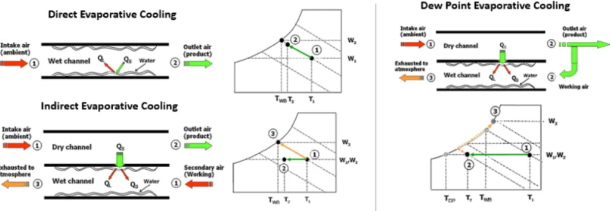
Evaporative cooling is a promising low energy alternative to vapor compression cool-ing systems. Unlike VCS, evaporative coolcool-ing is not bounded by Carnot efficiency since the refrigerant (water) delivers its cooling effect directly and operates in an open cycle rather than a closed cycle. Under the right climate conditions, evaporative cool-ing can reduce energy consumption by as much as 70% relative to conventional VCS. [37] The simplest form of evaporative cooling is direct evaporative cooling (DEC), in which water is evaporated directly into the airstream used for cooling the conditioned space (known as the process airstream). In the most common form, water drips slowly onto a wetted media and spreads by "wicking" on the surface and capillary action through the media. Air flows through the wetted corrugated channels, cooling it as water evaporates. The process is adiabatic, so all sensible heat lost by the air is gained as latent heat. This implies the upper limit for sensible cooling in a DEC is the wet bulb temperature. DEC performance is measured by wet bulb effectiveness -eqn. 1.6.

𝜂𝑤𝑏=

𝑡𝑖𝑛− 𝑡𝑜𝑢𝑡

𝑡𝑖𝑛− 𝑡𝑤𝑏

(1.6) In recent years, many empirical [40], numerical [11], and experimental [32][43] studies have been conducted to characterize performance of DECs, finding effective-ness up to 95% is feasible. The primary benefits of DEC are simplicity and efficiency, since there is only a single airstream, the only electrical power demand is a single fan and low-flow water pump. In dry regions where wet bulb temperatures are low, DEC

is an attractive option. In many humid climates however, DECs cannot satisfy ther-mal comfort for both temperature and humidity. Furthermore, the evaporative pad presents hygienic concerns if not maintained properly. Indirect evaporative cooling (IEC) systems use a second airstream, called the working air, to evaporate into, then transfer heat from the process air to the working air through sensible exchange with-out humidifying the process air. Unfortunately, the wet bulb effectiveness of these systems suffers due to the additional heat exchange step, and is generally limited to 40-60%. [37]

Dew point evaporative cooling, also known as M-cycle cooling after its inventor Valeriy Maisotsenk, is similar to IEC but instead of the working stream being supplied by ambient air, air from the dry channel is diverted to the wet channel after first being sensibly cooled in the dry channel. Only a fraction of the process stream air is cooled, but the air may be cooled below its wet bulb temperature, theoretically down to the dew point. Dew point evaporative cooling can reach dew point effectiveness (defined the same as eqn. 1.6, but with Twb replaced by Tdp) between 0.6-0.85 depending

on inlet conditions. [37] As with DEC and IEC, dew point cooling has the greatest capacity in dry climates.

Figure 1-8: Flow and process diagrams for DEC, IEC, and dew point cooling

1.2.4

Desiccant Dehumidification

As discussed in 1.2.1, modern vapor compression technology is inefficient at meeting latent loads in air conditioning. Desiccant dehumidification is an alternative approach

to remove moisture from air. Desiccant dehumidification comes in two forms - solid desiccant systems and liquid desiccant systems. This method relies on substances with low vapor pressure at their surface to pull moisture from the air by adsorption (solid desiccant) or absorption (liquid desiccant). A cycle is required to regenerate the desiccant once it is saturated, enabling continuous drying. The steps are as follows.

1. Sorption - desiccant begins dry and cool, its low vapor pressure draws moisture from the air, sorption may continue until the surface vapor pressure equals that of the air it is exposed to.

2. Desorption - the desiccant is heated and placed in a separate airstream. The heating increases its surface vapor pressure allowing moisture to be drawn out by the regeneration stream

3. Cooling - after moisture has been released and the desiccant is dry, it must be cooled to return it to a state of low vapor pressure so the cycle can continue.

Numerous configurations of dehumidifcation systems exist for both liquid and solid desiccant types. Figure 1-9 shows four types commonly used. Solid desiccant systems include the desiccant wheel (top left) and packed bed (bottom left) type. In a desiccant wheel, the solid desiccant is embedded in a honeycomb, forming channels parallel to the axis of rotation. The wheel rotates between a process and regeneration air-stream. This type has the advantage of high surface area and low pressure drop, but does not lend itself well to compact systems. The packed bed style consists of two "towers" with loose beads of desiccant. Air is alternated between the two beds by switching valves at the inlet and exit. Liquid desiccant systems include spray towers (top right) and liquid air membrane energy exchanger (LAMEE) systems (bottom right). In both systems the liquid desiccant is pumped between process and regeneration stages, the difference is in how the moisture exchange occurs. In spray tower systems, the liquid desiccant is sprayed through nozzles near the top of the vessel forming a mist. As the mist falls, air flows up against the direction of flow, allowing absorption or desorbtion to occur. This method has the advantage of favorable mass

transfer characteristics due to high surface area, but may allow entrainment of the desiccant into the air-stream. [24] LAMEE systems use membranes with microscopic pores which allow water to pass but prevent carryover of the desiccant. LAMEEs come in forms similar to conventional heat exchangers: shell-and-tube and flat plate. The shell-and-tube style consist of a bundle of hollow fibres in a shell. These offer impressive surface area to volume ratios as high as 2000 m2_/m3_{. Flat plate style}

LAMEEs are also common, and consist of alternating layers of air and fluid passages. These can be configured in parallel, crossflow, or counterflow orientation [45].

Figure 1-9: Solid and Liquid Desiccant Dehumidification Systems [24] [45]

1.2.5

LAMEEs

LAMEE performance, configuration, and design is an active area of research and much progress has been made in recent years to move these devices toward widespread use. Bai [6] constructed a LAMEE and studied its experimental performance using CaCl2

liquid desiccant. The effects of solution concentration, mass flow ratio, NTUs of the exchanger, and inlet temperature were considered. Max total effectiveness was found to be 0.53, and improved with lower inlet solution temperature. Li [30] conducted a numerical study of a dehumidifier with LAMEE exchangers, looking at many of the same parameters and optimizing for overall system effectiveness. They found NTU and mass flow rate ratio (m*_{) to be the most important driving parameters, and that}

effectiveness does not improve substantially beyond NTU = 2 and m* = 4.

Wang [42] quantified the thermodynamics of the ideal liquid desiccant dehumidi-fication cycle and explored the implications for efficiency limits at different operating conditions through energy and exergy analysis. A similar method is used for the re-generation energy calculations for the ideal cycle studies in Chapter 2. A run-around membrane energy exchanger RAMEE consists of two LAMEEs used together as an enthalpy recovery device. RAMEEs provide no cooling of their own but assist an existing HVAC system by recovering energy of make-up air. Kassai [27] numerically investigated the performance of a run-around membrane energy exchanger (RAMEE) and found up to 95% total effectiveness is possible, and an ideal Cr* _{of 3.2 for optimal}

system performance where Cr* is liquid desiccant capacitance over air capacitance.

1.2.6

Liquid Desiccant Cooling

Liquid desiccant dehumidification and evaporative cooling may be combined to cre-ate a liquid desiccant air-conditioning system (LDAS). LDAS has significant energy-saving potential since the cycle is primarily heat-driven in contrast to the work-driven vapor compression cycle. Desiccant dehumidification enables effective evaporative cooling in climates that would otherwise be too humid for it, and boosts the capacity of evaporative cooling alone. Kumar [29] investigates desiccant selection for an LDAC

system, considering LiCl, CaCl2, LiBr, and KCOOH in a simple liquid desiccant

cool-ing circuit with storage. LiBr was preferred in spite of 30% higher initial cost than LiCl due to its lower operating costs. Xiong [44] developed a novel two-stage liquid desiccant dehumidification system using LiCl and CaCl2 to assist the

dehumidifica-tion. This system reduces exergy loss in heat recovery and reduces the irreversibility of the process by pre-dehumidifiying with CaCl2. The study found nearly three-fold

thermal COP improvement from 0.24 to 0.73 and energy storage density of 237.8 and 395 MJ/m3 _{for CaCl}

2 and LiCl respectively. Cheng [14] explored the possibility of

an electrodialysis regenerator to enable regeneration of the liquid desiccant even in hot and humid environments. They found ideal performance of such a system gives a COP over 7 when conductivity of the liquid desiccant is high. Kozubal [28] devel-oped and patented a novel desiccant enhanced evaporative air conditioner (DEVap), which combines dew point evaporative cooling and liquid desiccant dehumidification. DEVap combines dehumidification and cooling into a single core which gives the ad-vantage of close thermal coupling between dehumidification (which requires a heat sink) and evaporative cooling (which requires a dry air source). The DEVap system claims 30-90% energy savings over conventional VCS technology without the use of harmful refrigerants. Figure 1-10 shows the physical core geometry of the DEVap system.

Figure 1-10: DEVap Cooling Core [28]

In many ways the DECAL system is similar to DEVap, but does not have direct thermal exchange between dehumidification surfaces and evaporative surfaces and uses direct evaporative cooling rather than dew point cooling - see section 2.3 for details.

Abdel-Salam [1] conducted a thermo-economic study of an LDAC system with solar regeneration in eight configurations varying the heating source and use of an energy recovery ventilator (ERV). They found the best system in terms of life cycle cost uses a solar thermal collector as the primary heat source, with natural gas as a backup and without an ERV. Life cycle cost was always lower when a solar thermal collector was included.

Chapter 2

System Design

The direct evaporative closed air loop (DECAL) system is a novel liquid desiccant cooling cycle designed to provide high efficiency residential cooling to meet rising demand. This chapter lays out the requirements for the system, walks through the thermodynamic cycle, and identifies the ideal performance limits of such a system relative to those in similar LDACs.

2.1

Figures of Merit and Design Constraints

The following conditions must be met to maximize the climate impact of a next generation high efficiency air conditioning system.

1. Reduced carbon footprint through improved efficiency

2. Widespread adoption in the marketplace

Cooling energy demand growth in the next 30 years will come primarily in resi-dential cooling [3]. The number of room air conditioners in use globally is expected to grow from around 1.2B today to 4.5B by 2050 [36]. Therefore the most impactful solution should fit in the residential size class - between 2 and 7 kW of cooling pro-vided. As shown in figure 1-6, the most efficient units available today in this range are mini-split systems with COP under 6. IEA studies [3] show mini-split systems

dominate the current and future residential global market, for this reason mini-splits are used as the benchmark incumbent system for this study.

Although LDAC systems show promise for substantial energy savings [28][44][31], none have yet been commercialized at large scale. The novel cycle proposed in this work seeks to overcome this obstacle by maintaining a balanced focus on both form and function to deliver a solution poised for widespread adoption. To this end, it is imperative to address building integration and consider the success of ductless mini split systems.

Split systems have the benefit of installation flexibility since only refrigerant lines connect the modules and the cooling modules deliver air directly to the conditioned space, eliminating the need for air ducts. This greatly simplifies installation and enables retrofitting into existing building stock without major renovation. Many modern split systems even offer "DIY" installation with pre-purged lines which require no specialized tools. This configuration also eliminates the parasitic loss of air drag in ducting, reducing fan power requirements and improving efficiency. As the name implies, split systems consist of multiple modules - typically an outdoor unit which includes the compressor and condenser, and one or multiple indoor evaporator units. This configuration further simplifies installation by splitting up the mass and volume of the device. While mini splits enjoy these practical advantages, they suffer the limitation that no air is exchanged between outdoor and indoor units. This limits their use in buildings with large make-up air requirements such as hospitals, office buildings, and shopping centers. In residential spaces there is enough natural infiltration from inhabitants ingress and egress and leakage to give adequate ventilation. In fact, limiting exchange provides an advantage since ventilation accounts for over half of all thermal losses in modern buildings [27]. As discussed in 1.2.1, the method of moisture removal in VC systems significantly reduces their efficiency, and desiccant based systems are well suited to handle moisture. This work seeks to answer the question: Can we design a liquid desiccant based air conditioner with the form factor advantages of a mini split system?

system is optimized to this design point.

Condition Value Units

Indoor dry bulb temperature 27 C Indoor relative humidity 60 % Outdoor dry bulb temperature 35 C Outdoor relative humidity 60 %

Cooling load 7 kW

Sensible heat ratio 0.75 W/W Table 2.1: Sizing Conditions Used In This Study

2.1.1

Physical Envelope

A survey of physical dimensions for Energy Star rated mini split units from [41] shows total system volume (indoor + outdoor unit) per Watt of cooling power. 1 _{For a}

high-efficiency system to be competitive it should be of similar size to current offerings, but with some allowance to acknowledge the efficiency benefits over incumbent systems. Therefore a target of 150 cm3_{/W is set. Furthermore, to facilitate transportation and}

maintain conventional building integration, the maximum dimension for all modules (except the solar thermal collector if used) is limited to 1m at the 7kW design point.

2.1.2

Thermal Coefficient of Performance

Unlike VC systems where most of the energy supplied is electrical power to the com-pressor, LDAC systems are thermally driven. Regeneration heat is required to con-centrate the desiccant after it absorbs moisture from the air. The thermal coefficient of performance is defined by equation 2.1 below.

𝐶𝑂𝑃𝑡ℎ=

𝐶𝑜𝑜𝑙𝑖𝑛𝑔 𝑂𝑢𝑡𝑝𝑢𝑡 (𝑊 )

𝐻𝑒𝑎𝑡 𝐼𝑛𝑝𝑢𝑡 (𝑊 ) (2.1)

Figure 2-1: Energy Star Split Systems Specific Volume

Regeneration heat can come from waste heat, solar thermal energy, or a heat pump. If solar energy is used, the size of the collector required depends on the thermal COP of the system, the relationship between incident solar irradiance and cooling load, and the storage capacity of the system. Detailed design of the solar thermal collector requires a more specific application which is beyond the scope of this study, but to keep collector size small the target COPthis set to 0.70. This target

is reasonable based on a survey of solar assisted desiccant evaporative cooling systems by Jani [26] in which COPth ranged from 0.25 to 1.38. 2

2.1.3

Electrical Coefficient of Performance

Electrical COP of the system is defined by equation 2.2 below.

𝐶𝑂𝑃𝑒𝑙𝑒𝑐 =

𝐶𝑜𝑜𝑙𝑖𝑛𝑔 𝑂𝑢𝑡𝑝𝑢𝑡 (𝑊 )

𝐸𝑙𝑒𝑐𝑡𝑟𝑖𝑐𝑎𝑙 𝐼𝑛𝑝𝑢𝑡 (𝑊 ) (2.2) As discussed in 1.2.1, COP for evaporatively cooled systems is not bounded by Carnot limits. Without the burden of a mechanical compressor, electrical COP can be quite high since the only power draw comes from fans, pumps and electronics.

2_{This study was a survey of solid desiccant systems rather than liquid, but the thermodynamic}

Coolerado [16] cites an electrical COP over 18 for the M50C series dew point evap-orative coolers. The global cooling prize [36] proposed an 80% reduction in energy consumption from a present day baseline COP of 3.5 is needed to offset the dramatic increase in demand coming in the next 30 years. A target electrical COP of 20 is used in this study.

2.1.4

Cooling Unit Airflow

The airflow required by the indoor cooling unit to meet a given sensible demand depends on the room temperature, the temperature of the cold air provided, and the density of the air. Indoor temperature is specified by the user and is therefore a function of human thermal comfort. Thermal comfort is dependent on dry bulb temperature and humidity, and AC cooling capacity is generally measured with indoor conditions near the upper limit of comfort. In the US, SEER testing calls for an indoor condition of 26.7C & 50.7% RH. For this study, an indoor condition of 27C and 60% RH is used. Furthermore, the sensible heat ratio is set at 0.75 unless specified otherwise. The sensible cooling is given by equation 2.3.

𝑄𝑠𝑒𝑛𝑠 = 𝑄𝑡𝑜𝑡SHR = ˙𝑣𝜌𝑐𝑝(𝑇𝑟𝑜𝑜𝑚− 𝑇𝑐𝑜𝑜𝑙) (2.3)

Where ˙𝑣 is the volume flow rate of air (𝑚3/𝑠), 𝜌 is the density of air (𝑘𝑔/𝑚3), 𝑐𝑝 is

the specific heat of air, 𝑇𝑟𝑜𝑜𝑚is the temperature of the conditioned space, and 𝑇𝑐𝑜𝑜𝑙is

the temperature of the cooling air provided by the indoor unit. For practical purposes such as noise, it is necessary to limit the volume flow of the indoor unit. A typical mini split system indoor unit flows around 3 𝑚3/𝑚𝑖𝑛/𝑘𝑊 so the cool air temperature of the cycle must be low enough to meet that flow - substituting into equation 2.3 and solving for 𝑇𝑐𝑜𝑜𝑙the required outlet temperature is 14.4C. Ideal cycle studies show

this target temperature is infeasible for the target condition. Commercially available evaporative coolers do typically require more airflow due to the smaller temperature difference between outlet condition and room condition. The target specific flow is set at 6 𝑚3/𝑚𝑖𝑛/𝑘𝑊 of cooling.

Table 2.2 summarizes the figures of merit used in this study.

Figure of Merit Target Units

System COPelec 20 W/W

System COPth 0.70 W/W

Specific Volume 150 cm3_/W

Indoor Unit Flow Rate 6 m3/min/kW Table 2.2: Figure of Merit Targets

2.2

System Overview

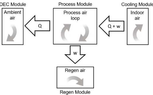
The DECAL system consists of four modules, the process module, DEC module, regeneration module, and cooling module. Each module serves an essential function to achieve the net effect of heat and moisture removal from the conditioned space. The modules are discrete in their function and may be co-located or physically separated as needed based on the physical limitations of the installation. Figure 2-2 shows a simplified block diagram of the system.

The DEC and regeneration modules reject heat and moisture to ambient air, and the cooling module captures heat and moisture with the indoor air. Liquid desiccant (LD) is pumped between modules and serves as the heat and mass transfer fluid for the system. A water supply from a water reservoir or municipal source is required for the DEC and process modules. Each module requires electrical power as well to run pumps and fans. However, there is no direct air exchange between modules, or between the indoor space and ambient air. In this way, the system is most similar to a distributed system like a chiller, in which a water or antifreeze solution circulates between the cooled space and a remote cooling system. Ductless mini-split systems offer similar flexibility, with refrigerant lines running between indoor evaporator units and an outdoor unit containing the compressor and condenser coil. In each case, the advantage is in having compact lines connecting modules, rather than large air ducts. Smaller lines are easier to retrofit into existing buildings, giving a practical advantage. There is also a cycle benefit to such systems, since parasitic heat gain on the lines is proportional to surface area, and line sizes may be dramatically smaller for systems circulating water, refrigerant, or liquid desiccant. Unlike the chiller or mini-split system, the DECAL system enables moisture removal through the circulated liquid desiccant. This allows the system to meet latent loads much more efficiently, avoiding the drawbacks discussed in section 1.2.1. There is no vapor compression cooling in the DECAL system - all cooling is provided by evaporation of water. There are two direct evaporative coolers (DECs) which operate on different air-streams to produce cooling. The system is designed to allow the DECs to produce an additive temperature effect. The first DEC acts on ambient air and is thus limited to the ambient wet bulb temperature. The second DEC acts on the closed air-stream which is cooler and drier than the ambient condition. This allows the system to reach temperatures below the ambient dew point, which is the limit for conventional evaporative cooling systems.

The DECAL system includes two liquid desiccant loops, the cooling loop and the process loop. Both loops use a common liquid desiccant - either LiCl or CaCl2 (both

are considered in this study). The LD process loop operates at high concentration and serves primarily to dry the process air-stream. The LD cooling loop operates

at mild salt concentration and provides both the sensible and latent cooling to the conditioned space. The two LD loops operate independently except for a mixing valve after the indoor cooling LAMEE in the LDC loop and after the process LAMEE in the LDP loop which allows the cooling loop to regenerate by trading a small volume of dilute solution with equal volume of strong solution from the process loop. In this way, only a single regeneration circuit is needed for both LD loops - see figure 2-3 for the full system diagram. The lower concentration of the LD cooling loop allows it to operate at cooler temperatures without risk of crystallization. It is also favorable to use a lower concentration in the cooling circuit to avoid over-drying the conditioned space. By metering the exchange between LDC and LDP loops, the concentration of the LDC stream may be controlled to give independent control of sensible and latent cooling and match the SHR of the conditioned space.

2.3

Cooling Cycle

The DECAL system provides all cooling power through direct evaporative cooling. As discussed in section 1.2.3, the lower limit of outlet air temperature in a DEC is the wet bulb temperature of the inlet air stream. In many climates, particularly in the tropics where future demand is greatest, the ambient wet bulb temperature is still above human comfort and thus DEC alone is inadequate. However, when combined with desiccant dehumidification, a staged evaporative cooling system may overcome this obstacle. In simplest form, a 2-stage direct liquid desiccant evaporative cycle would consist of three steps.

1. Stage 1 DEC from ambient

2. Desiccant dehumidification in a LAMEE 3. Stage 2 DEC from the dry condition

Here we assume both evaporative processes are constant enthalpy, and that the stage 1 DEC cools not only the process air stream, but also the liquid desiccant used

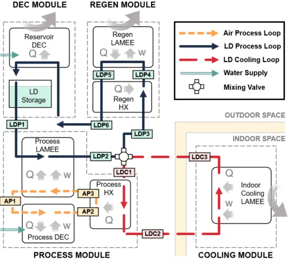
Figure 2-3: Full System Schematic

for dehumidification. In an ideal counterflow LAMEE, most of the heat of adsorption goes to the liquid desiccant stream [22], so process 2 is isothermal. The overall cooling effect depends on the ambient wet bulb, which sets the cooling capacity of stage 1, and the liquid desiccant equilibrium vapor pressure (a function of mass concentration and temperature, see 3.5.2), which sets the capacity of stage 2. At the limit, the maximum achievable capacity of stage 2 is set by the saturation limit of the liquid desiccant used in the cycle. Figure 2-4 shows an ideal two stage evaporative cooling cycle using CaCl2 from an ambient condition of 35C & 60% RH. At this climate condition even

an ideal DEC cannot provide cooling in a single stage since ambient 𝑇𝑤𝑏 is above

the room temperature. However, with a 2-stage system an outlet condition of 17C is possible.

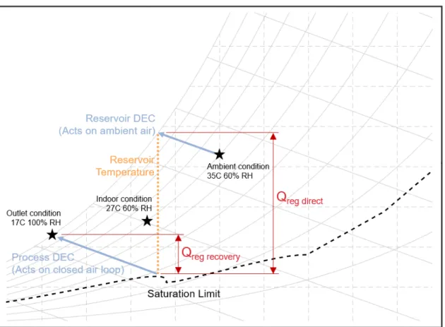
In a direct 2-stage system, a single air stream supplies cooling directly from the ambient condition. Wang [42] showed the ideal regeneration energy is proportional to the net water vapor absorbed by the system. So in a direct 2-stage system, the regen-eration heat scales with the difference between the ambient wet bulb humidity and the saturation limit humidity at reservoir temperature. The thermodynamic advantage of the DECAL cycle comes from the use of recirculated air in a closed loop rather than ambient air. This allows the system to recover much of the dehumidification energy which would otherwise be lost in a direct supply system. The DECAL system only needs to regenerate the moisture gain from the stage 2 DEC, while a direct system needs to regenerate moisture gain from both stages, as well as the difference between the supply air condition and the ambient condition humidity.

Figure 2-4: DECAL Staged Evaporative Cooling

In this way the DECAL system is able to provide sensible cooling well below the ambient dew point by evaporative means alone, and minimize the regeneration

energy required for continuous operation. DECAL uses direct evaporative coolers rather than more sophisticated evaporative cooling systems such as indirect-direct or dew point cooling. The rationale for this choice is driven by two factors. Dew point coolers require a second working air stream with similar mass flow to the process stream. This requirement is incompatible with the closed air loop since all air in the loop must be recycled, so the working stream would need to be pulled from ambient, increasing the regeneration heat required. A dew point cooler could be used in place of the reservoir DEC, however volume constraints make this inadvisable. Both dew point and indirect-direct coolers transfer heat between two air streams. Air-to-air heat transfer requires large surface areas to be effective, and would make the system less competitive on specific volume.

2.4

Air Process Loop

The closed air loop is the heart of the DECAL system. Air flows between three exchangers in the process module to provide sensible cooling to the liquid desiccant cooling loop. The cycle begins at the inlet to the process DEC just after exiting the process LAMEE (AP1). At this condition the air has been dried well below ambient humidity (around 20% RH at the design condition). Air enters the direct evaporative cooler and is sensibly cooled to near its wet bulb temperature (AP2). This is the coldest point in the cycle and must be well below the room condition for the cycle to be viable. The cold air then enters the process HX where it picks up heat from the LDC stream and warms back up near (but below) the room temperature (AP3). At this point the air returns to the process LAMEE where it transfers the moisture gained in the DEC to the LDP stream and begins the cycle again. Depending on the relationship between ambient wet bulb temperature and room condition, AP3 may be slightly warmer or cooler than AP1. Figure 2-5 shows the relevant sections of the cycle on the psychrometric chart and on the system diagram.

Figure 2-5: Air Process Loop Cycle and Diagram

2.5

LD Cooling Loop

The LD cooling circuit provides sensible and latent cooling to the indoor space. It is the DECAL equivalent of the evaporator in a conventional VC system. Liquid desiccant flows between the indoor and outdoor space through small pipes (less than 1" diameter). The process begins at the process heat exchanger inlet (LDC1) where sensible heat from the cooled space is transferred to the process air stream, cooling the LD stream without changing its mass concentration (LDC2). After cooling, the LD enters the indoor cooling LAMEE, where it takes both heat and moisture from the cooled space, heating it and reducing its mass concentration of liquid desiccant (LDC3). The LDC stream is heated beyond the sensible heat transferred from the cooling air due to the heat of absorption from the latent transfer. The LD then enters the mixing valve where a small volume (less than 5% of total flow) is transferred between streams. Since the LDP stream always operates at higher mass concentration than the LDC stream, this regenerates the LDC stream and dilutes the LDP stream. A small amount of heat is generated when the stronger LDP stream flow mixes with the LDC stream flow (enthalpy of dilution) however, since the total mass transferred is small relative to the total flow, this effect is negligible. Figure 2-6 shows the relevant sections of the cycle on the psychrometric chart and on the system diagram.

Figure 2-6: LD Cooling Loop Cycle and Diagram

2.6

LD Process Loop

The LD process loop carries the moisture from the process DEC and latent load removed from the conditioned space to the regeneration LAMEE where it is released outside, allowing the system to operate continuously. The process begins with liquid desiccant exiting the LD storage tank where it has been cooled by the reservoir DEC near the ambient wet bulb temperature (LDP1). At this point the LD is concentrated and at the lowest temperature in the cycle, so its margin to the solubility limit is smallest. The design point condition for solubility margin is set to 5%, so the mass concentration at this point is 95% the concentration at which it would begin to precipitate from solution. For CaCl2 this is around 0.47 g/g and for LiCl this is around

0.44 g/g. The LD enters the process LAMEE where it dries the process air, diluting the solution and heating due to heat of absorption (LDP2). The LDP stream is then diluted by mixing with the LDC stream at the mixing valve (LDP3). It then enters the cold side of the regen heat exchanger, or economizer, which recovers some of the heat required for regeneration. Since this heat exchanger is between two liquid desiccant streams, the heat transfer coefficients are high and the heat exchanger may be quite compact. After the economizer, the LD is further heated from the regen heat source (solar thermal collector or waste heat) to reach LDP4. The air regeneration stream

(AR) is pulled from ambient and heated to match the temperature of LDP4, then both streams enter the regen LAMEE at the same temperature for regeneration. Moisture is removed from the LDP stream and enters the AR exhaust stream (AR2). The process of desorbtion is endothermic and cools the LDP stream (LDP5). The LD then enters the hot side of the economizer and transfers heat to the cold stream (LDP6). Finally LD is cooled back near ambient wet bulb temperature by the reservoir DEC and enters the LD storage tank, this closes the cycle.

Figure 2-7: LD Process Loop Cycle and Diagram

2.7

Ideal Cycle Limits and Benchmarking

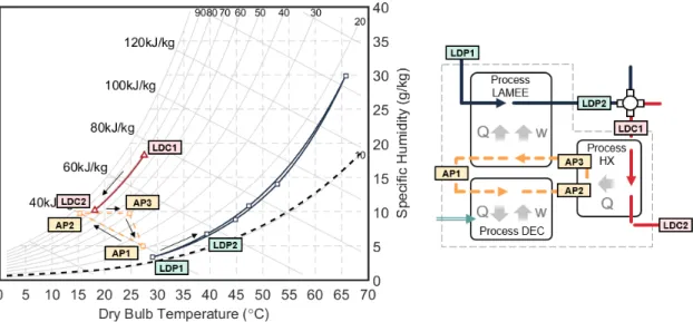
To validate the claim that the DECAL cycle offers thermodynamic advantages over direct supply systems, the ideal cycle performance of several similar systems was eval-uated. System 1 comprises a single drying LAMEE followed by a direct evaporative cooler. Ideal performance is assumed for both the LAMEE (sensible and latent ef-fectiveness) and DEC (wet bulb efficiency), and the drying LAMEE inlet condition is set at the solubility limit of the liquid desiccant at the inlet temperature. System 2 consists of a drying LAMEE followed by a dew point cooler (M-cycle). The wet bulb effectiveness is set to 1.20 based on the work of [37] and the ratio of process

air to working air is 1:1. The working stream air for system 2 must also be dried, so the regeneration requirements are doubled relative to a direct evaporative system. However, system 2 does have the advantage of cooler outlet temperatures since it can cool beyond the wet bulb temperature. System 3 is the DECAL system described in this work, with ideal exchanger effectiveness on all exchangers. Indoor temperature is set to 27C and max allowable indoor RH is 60%. The SHR is 0.75. The max indoor RH and SHR imposes an upper limit for systems using direct evaporative cooling. In cases where the cooling stream wet bulb condition falls above the condition line, cooling was limited to the intersection such that SHR is met and the indoor RH is 60%. In cases where the outlet condition falls below the condition line (this mostly applies to system 2) the indoor RH is lowered. This is representative of what would actually occur if latent cooling exceeds the latent load, but does suggest that a dew point cooler system could operate with less drying than shown here.

Each system in the study was assessed both with and without a DEC pre-cooling stage (reservoir DEC in the DECAL system). The ideal thermal coefficient of per-formance was found for each system using both CaCl2 and LiCl, and over a broad

range of ambient conditions (30-45C dry bulb temperature and 20-80% RH). Figure 2-8 shows system diagrams for the process side of each system evaluated, and the cycle of each system on the psychrometric chart at the design condition.

The results are promising for the DECAL system (System 3 with precooling). Figure 2-9 shows contours of the thermal COP limits for each system over the range of ambient conditions evaluated. As expected, performance degrades at higher tem-peratures and humidities, with some systems falling off faster than others. In general, systems 1 and 2 perform well at very low relative humidity (under 30%). However, at these dry conditions evaporative cooling systems may be used without a desiccant, so performance at higher humidity is of greater interest. DECAL shows capability im-provements over much of the range of interest, especially at high ambient temperature and humidity. Both systems 1 and 3 use direct evaporative cooling, so systems with a single stage are limited to the wet bulb temperature corresponding to the solubility limit of the desiccant and ambient temperature. For CaCl2 this occurs just under 40C

Figure 2-8: System Diagrams for Ideal Limits Studies

ambient dry bulb, so these systems are not viable above that condition, regardless of humidity. Direct comparison between CaCl2 and LiCl shows that with precooling,

often CaCl2 outperforms LiCl. This was unexpected since LiCl offers superior drying

capacity. It implies that there is an optimal condition at which additional drying is not advantageous i.e. the incremental improvement in cooling capacity over the incremental additional regeneration heat has a maximum. This does not necessarily suggest that CaCl2 will outperform LiCl in a real system since LAMEE latent

effec-tiveness will reduce the actual drying capacity possible, and the lower vapor pressures LiCl offers would allow a smaller exchanger to be used.

While the findings of this study show great promise for the DECAL system, they are incomplete, since actual system performance will vary significantly from the ideal limit. The DECAL system is more complex than the two benchmarks systems it is compared against. This will put more restrictive limits on its performance when component inefficiencies are considered. Actual system performance is investigated extensively with the full system performance model detailed in Chapter 3.

Chapter 3

Mathematical Model

To simulate system performance, a mathematical model is created using Matlab. The model takes inputs for the indoor and outdoor climate, sensible heat ratio, imposed component efficiencies, liquid desiccant composition (LiCl or CaCl), relative flow rates for each of the fluid loops, and selected geometry constraints. Outputs include cooling power provided, thermal energy and temperature required to regenerate the desiccant, electrical power draw of fans and pumps, and volume required for each exchanger to meet the set efficiencies. The first goal of the simulation is to understand the system limitations with realistic component efficiencies relative to the state of the art. The second goal is to gain insight into the trade-offs between component efficiencies, volume, power, and flow constraints to design a well balanced system. The model is built with a layered architecture of routines and subroutines designed to provide robust and accurate results while maintaining flexibility and speed. Figure 3-1 gives the top-level model architecture for the Matlab model.

The optimization wrapper allows the user to run design studies for various inputs. These inputs may be either boundary conditions such as climate, design parameters such as exchanger efficiencies, or operational settings such as relative flow rates of the fluid loops. The main loop is used to run a single design point. It may be run either as a function called by the optimization wrapper or alone if solving for a single condition. The main loop sets all static parameters needed to solve the system, sets initial guess values for the solver, calls the solver routine, and executes some post-processing