Analysis and design of a two-axis noncontact position sensor

Analysis and Design of a Two-Axis Noncontact

Position Sensor

by

Robert John Ritter

Submitted to the Department of Mechanical Engineering

in partial fulfillment of the requirements for the degree of

Master of Science

at the

MASSACHUSETTS INSTITUTE OF TECHNOLOGY

February 1999

©

Massachusetts Institute of Technology 1999. All rights reserved.

11 A ~-' I

Author ...

Department of Mechanical Engineering

January 30, 1999

Certified by...

David L. Trumper

Rockwell International Associate Professor of Mechanical Engineering

Thesis Supervisor

A ccep ted b y ...

Ain A. Sonin

Chairman, Department Committee on Graduate Students

Analysis and Design of a Two-Axis Noncontact Position

Sensor

by

Robert John Ritter

Submitted to the Department of Mechanical Engineering on January 30, 1999, in partial fulfillment of the

requirements for the degree of Master of Science

Abstract

This thesis presents the design, analysis and construction of a two-axis noncontact position sensor. We use this sensor in a magnetic levitation stage where we levitate a 0.64 mm (0.25 inch) diameter, 1 mm (0.04 inch) wall steel tube. The sensor has a circular opening approximately 13 mm (0.5 inch) in diameter through which the tube passes.

A three-pole arrangement with a three-phase input current generates a flux which

changes as a function of the tube position. We model the sensor with a magnetic circuit and use this model to predict the relationship between the tube position and the flux behavior. We then use a signal processing board to convert the raw output from the sensor into two voltages, dependent on the x and y position of the tube, respectively.

In this thesis we also describe the design and construction of a three-phase signal generator which drives the three-phase field, the operation of the closed-loop current supply, and the design and construction of the signal processing board.

Thesis Supervisor: David L. Trumper

Acknowledgments

First of all, I have to express my sincerest gratitude to my thesis advisor, Professor David Trumper. His guidance and direction have made my time here at M.I.T. more profitable than I ever imagined. Often a two-minute analysis by Professor Trumper would solve a problem on which I had spent hours. I will always remember my time as a student of his, and I am proud to have been one of his advisees. Along with Professor Trumper, Ming-chih Weng has not only been endlessly patient with me as a Master's student, but has been a great friend as well. I cannot imagine a better person to work with. Thanks Ming.

I also must thank all my friends in the Precision Motion Control laboratory for

making me feel welcome from the first time I set foot in the lab. I can easily say that the people of the PMC lab are the most intelligent group I've ever had the honor to learn with. Even at it's fullest, the lab has always been a good place to be. I regret that my friends David Ma, Claudio Salvatore and Paul Konkola were not here for the duration of my stay, but I enjoyed knowing them while they were here. Stephen Ludwick has disproven every negative stereotype imaginable about MIT students, and was always willing to stop his work to help me solve a problem. I have yet to find a question to which Pradeep Subrahmanyan does not know the answer, and I'm grateful for all the help he has given me on everything from electric fields to control systems. Mike Liebman has an incredible amount of talent, and I will always remember him as someone who, quite simply, gets things done. David Chargin, my fellow UC Davis graduate, has been a good friend with whom I can discuss not only research issues but life issues as well. I thank Joe Calzaretta for sharing with me his

intrinsic joy of knowledge and for being such a good friend.

And I have to thank Gerry Wentworth and Mark Belanger for their patience and help with building the hardware. I always feel comfortable asking either of them for help; Mark has a great way of educating people without making them feel completely ignorant, which can be a tough thing to do considering the level of ignorance most of us have when in the machine shop! Maureen Lynch and David Rodriguerra have

kept me on track with more things than I can remember, and have been very patient with all of us in the PMC lab.

I also must thank the National Science Foundation for funding this research. I

am proud to be part of such a program.

I would never have made it this far without my mother and sister. Mom, Launi,

thank you so much. Education has always been my mother's highest value and I know that her attitude has everything to do with my progress as a student. I can not express enough the strength I have gained from knowing I have Launi and my mother always willing to help in any way they can.

And finally to my Fiancee, Larissa, who has shown me how wonderful life can be.

I know that this last 18 months I spent far too much time in the Lab, but Larissa

always supported me with her love and warmth. I look forward to our lives together with great joy.

Contents

1 Introduction

1.1 Overview. . . . . 1.2 Background . . . . 1.2.1 Sensor . . . . 1.2.2 Actuator and Controls . . . .

1.2.3 Results . . . .

1.3 Thesis Layout . . . . 2 Background Theory

2.1 Notation . . . . 2.2 Maxwell's Magnetoquasistatic Equations

2.2.1 MQS Assumption . . . .

2.2.2 Example Problem . . . . 2.2.3 Transfer Functions . . . 2.3 Magnetic Circuit Analogy . . .

2.4 Magnetic Diffusion Equation . . 2.4.1 Skin Depth . . . . 2.4.2 Attraction or Repulsion 2.4.3 Shielding . . . . 3 Sensor Development 3.1 Introduction . ... 3.2 LVDT . . . . 3.2.1 Operation . 3.2.2 Terminal Rel 3.3 E-Pickup . 3.3.1 Experimental 3.4 Modified E-pickup .t.n... ations . . . . E-Pickup Setup ... .. .. . . . . . .

3.4.1 Experimental Data From Modified E-pickup

3.5 Final Design . . . .

4 Field Analysis

4.1 Introduction . . . . 4.2 Magnetic Circuit Analogy . . . . 4.2.1 System Model . . . . 21 . 21 . 22 23 26 27 31 33 34 34 34 35 38 39 42 43 46 51 55 55 56 56 57 62 66 67 72 74 77 77 77 78 . . . .

4.2.2 Circuit Analysis . . . . 79

4.2.3 Solving the Magnetic Circuit . . . . 84

4.2.4 Output Voltage As A Function Of Tube Position . . . . 88

4.2.5 Tube Position As A Function Of Output Voltage . . . . 91

4.2.6 Experimental Data From Three-Phase Sensor . . . . 94

4.3 Exact Solution With Tube Centered . . . . 99

4.3.1 Vector Potential. . . . . 101 4.3.2 Boundary Conditions . . . . 104 4.3.3 Field Solution . . . . 110 4.4 Summary . . . . 115 5 Electronics 117 5.1 Introduction . . . . 117

5.2 Three Phase Signal Generation . . . . 117

5.2.1 Clock and Counter . . . . 120

5.2.2 EPROM . . . . 120

5.2.3 Digital to Analog Converters . . . . 121

5.2.4 Board Layout . . . . 123

5.3 Current Supply . . . . 125

5.3.1 Low-Pass Filter . . . . 126

5.3.2 Primary Coil Load . . . . 127

5.3.3 PA-12 Power Amplifier . . . . 128

5.3.4 Feedback Loop . . . . 129

5.3.5 Choosing Component Values . . . . 130

5.4 Signal Processing Circuit . . . . 131

5.4.1 Rectification. . . . . 132 5.4.2 Summing Junctions . . . . 134 5.4.3 Low-Pass Filter . . . . 134 5.4.4 Output Gain . . . . 135 5.4.5 Circuit Layout . . . . 136 6 Construction 141 6.1 Introduction . . . . 141 6.2 E-pickup . . . . 141 6.3 Modified E-pickup . . . . 142 6.4 Three-Phase Sensor . . . . 142 6.4.1 Lamination Pieces . . . . 143 6.4.2 Coil Winding . . . . 145 6.4.3 Shielding. . . . . 146

6.5 Rail Mounting System . . . . 147

6.5.1 Sensor Mount . . . . 147

7 Conclusions and Suggestions for Further Work 149

7.0.3 Experimental Issues . . . . 149

7.1 Closing Thoughts . . . . 151

7.2 Suggestions for Further Work . . . . 151

A Matlab Code 153 A.1 Magnetic Vector Potential and Field Lines . . . . 153

A.1.1 Case 1: Uniform Field . . . . 153

A.1.2 Case 2: Fourier Series Field . . . . 157

List of Figures

1-1 Photograph of one of the quartz ovens which cure the paint on the tube. The tube diameter is approximately 22 mm. A levitation station can be seen behind the oven. . . . . 23

1-2 Two levitation stations spaced approximately 3.5 meters apart stand on either side of an induction heater. The electrostatic powder paint coating station is just visible at the far right. The tube moves from right to left in this picture at a velocity of 1-2 m/sec. . . . . 24

1-3 Benchtop scale model showing five sensor and actuator pairs. We use an aluminum rail to position the components. As shown in the photo, the position of the sensor relative to the actuator alternates down the length of the setup... 25

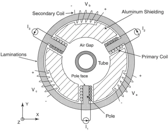
1-4 Layout of the noncontact position sensor. Three current sources each drive a primary coil, which creates a flux read by the secondary coils. The flux paths, and thus the voltages induced on the secondary coils,

are functions of the tube position. . . . . 26 1-5 Photograph of the noncontact position sensor. The outer ring and inner

shapes are aluminum shielding. We wrap the laminations in Teflon tape to prevent scoring the edges of the coil wire (creating a short circuit from scraping off the insulation); the laminations are therefore white in this photo. We pot each coil in epoxy for increased rigidity and resistance to scoring. . . . . 27 1-6 Photograph of the signal processing board. The BNC output jacks

connect to the control computer. We can tune the output voltages using the potentiometers on either side of the jacks. . . . . 28 1-7 Experimental hardware, including the sensor, the signal processing

board, and the mounting hardware. The metal bracket is aluminum, and the translucent bracket is plexiglass. . . . . 28 1-8 Trace of path followed by the tube relative to the sensor which we use

to estimate the linearity of the sensor output. The tube is held fixed and the sensor is moved around it so that the relative motion is as suggested by the lines in black. We then repeat this exercise for the x-direction using a similar but horizontal pattern. . . . . 29

1-9 Trace from the oscilloscope showing experimental data. The trace

shows the x- and y-voltages output from the signal processing board plotted against each other as we move the tube and sensor relative to each other as shown in Figure 1-8. The ideal output is an exact trace of the path in Fig. 1-8. . . . . 30

2-1 Example magnetic circuit. A voltage V across the primary coil drives a flux which links the secondary coil. We assume the air gap is small enough that we may ignore the fringing of the field. . . . . 36

2-2 Magnetic circuit element representation of the example problem. The resistive and voltage source elements model the behavior of the sensor, allowing us to solve for the terminal relations using traditional circuit analysis m ethods. . . . . 41

2-3 Field Hx' incident upon a conductor. Because of the conductivity, an

opposing field is created in the conductor to repel the original field, thus limiting the penetration of the imposed field into the conductor. 44 2-4 Skin depth of a magnetic field in a conductor. On the j 0 edge, the

induced field inside the conductor instantaneously equals the applied

H field. The imposed field varies sinusoidally with time; the field in

the conductor is a traveling wave. . . . . 45

2-5 Permeable, conducting, hollow cylinder in a uniform, time-varying field

imposed as the vector potential at surface (e). We assume no variation in the z-direction, and finite permeability and conductivity in the tube region . . . . 48

2-6 Field lines for a steel tube. The imposed field has frequency ~ 0 Hz;

this is the DC case. We impose a sinusoidal vector potential along the outermost surface and use the transfer relations to calculate the distribution throughout the regions. . . . . 49

2-7 Field lines for a steel tube with an imposed field frequency of 5 kHz.

The field inside the tube is now concentrated near the surface, but the field in the air-gap is similar to the DC case above. . . . . 50 2-8 Field lines for a steel tube with an imposed field frequency of 100 kHz.

The field in the tube continues to concentrate in a thinner layer of the

tube while the field in the air-gap remains essentially the same. . . . 50

2-9 Field lines for an aluminum tube with an imposed field frequency of 100 kHz. We plot this case as a check on our solution, and we see the

conductor repels the field as we expect. . . . . 51

2-10 Various flux paths: 1) through air-gap, 2) entering pole mid-way, 3) through secondary coil. Paths 1) and 2) are acceptable, but path 3) is not. ... ... ... 52 3-1 Cross section of a cylindrical LVDT. We assume the flux <D travels

directly from the highly permeable piston to the highly permeable outer core. ... ... 57

3-2 Schematic of a cylindrical LVDT, and associated radial field at the outer surface of the piston as a function of position. . . . . 57 3-3 Close-up of LVDT secondary coil. For the local axes we define the

z = 0 point at the tip of the piston for computation of the flux linked by the secondary coil. . . . . 61

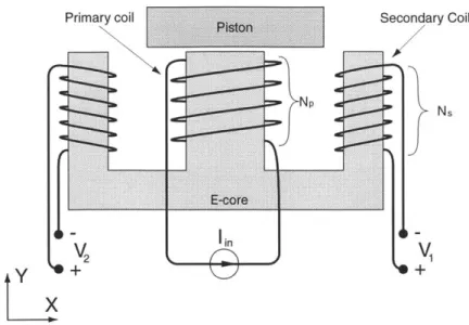
3-4 E-core schematic. A current supply drives the primary coil to create a flux dependent upon the piston position. The piston moves in the x-direction only. . . . . 63 3-5 Schematic of E-pickup sensor with magnetic circuit overlay. We lump

all the leakage flux into a single term, however in the actual sensor there is leakage flux along the entire height of the poles . . . . 64

3-6 Circuit diagram of the E-pickup sensor. Representing the magnetic

elements with MCA equivalents allows us to use Kirchoff's laws to calculate the flux. . . . . 64

3-7 E-core without coils. We use electrical tape to prevent scoring the coils

on the square edges of the ferrite, and we mount the sensor in plastic to minimize the effect of the mount on the field distribution. . . . . . 67 3-8 Physical dimensions of E-core used in first experiment. The depth into

the page (in the z-direction) is 19 mm. . . . . 68 3-9 Experimental output from E-pickup sensor. Increasing the tube height

from 0.5 mm to 1.5 mm decreases the sensitivity by about half. . . . 68

3-10 Schematic of second E-core sensor. The secondary poles are now above

the tube to give a different flux path. The depth of the sensor in the z-direction is 20.4 mm . . . . 69 3-11 Modified E-pickup with copper shielding. The wires at the bottom of

the photo are shielded in aluminum. . . . . 70 3-12 Result of demodulating a shifted sinusoid. The input signal is sin(0

-00), and the reference is sin(0). We show the case for 00 = 1 radian. If 00 were I radians, the DC component would be zero. Also note the₂ primary frequency is now twice the original. . . . . 71 3-13 Experimental data from the modified E-pickup sensor without

shield-ing, showing output voltage vs. lateral displacement. The legend shows tube height above primary pole face; we take each series of data at a different height as noted in the legend. The data series tend to spread towards the edges of tube travel . . . . 72

3-14 Experimental data from the modified E-pickup sensor with shielding in place. Apart from the case at height 1 mm which is close to linear in both cases, the output is more uniform, with less deviation as the tube nears the edges of the sensor range. The difference is much more dramatic if we ignore the data series for the 1 mm case. . . . . 73 3-15 Experimental data from the modified E-pickup sensor comparing shielded

case with unshielded case for tube heights of 1 mm and 9 mm. The 1 mm data series follow each other closely, with primarily a DC offset. The 9 mm series tend to differ more towards the edges of measurement. 73

3-17 Photograph of position sensor. . . . . 7 4-1 Equivalent magnetic circuit of the sensor. We assume the shielding will

constrain the flux to the paths above; which we denote as reluctances, R . . . . 7 8

4-2 Simplified magnetic circuit. The delta-wye transformations allow us to reduce the ten reluctances of the previous circuit to three. . . . . 80

4-3 Geometry for calculating a lumped-parameter reluctance. The shaded area is the area over which we integrate to find an exact solution. The cross-hatched area is the rectangular approximation. . . . . 81

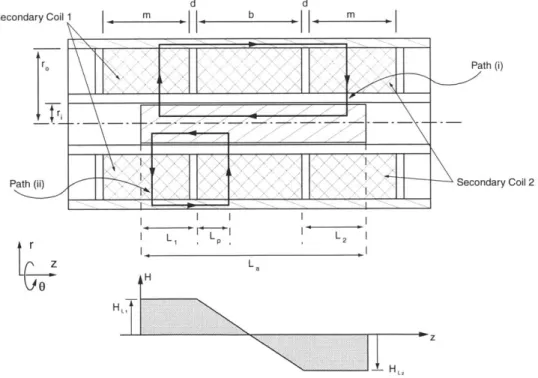
4-4 Cutout of center of sensor showing the geometry we use to calculate the lumped parameter reluctances. The cross-hatched area represents the aluminum shielding, shaded areas RLB and R7t represent the as-sumed flux paths. The dimension w, is one-third of the lamination pole thickness. . . . . 83

4-5 Phasor components of fluxes through poles 1, 2 and 3 normalized to

' R 2 +R 'Z 3 +R31I. We see from the symmetry of the phasors that D1 +

(D2 + D3 = 0, as we expect from driving the sensor with a three-phase

signal. . . . . 86

4-6 Flux 4

DB (in black) and corresponding components (in grey),

normal-ized to -,; along with output voltage VB normalized to -- - We

show the case for the tube in the center of the sensor such that the

reluctances RAeq,Beq,Ceq are all equal. . . . . 89

4-7 Geometry for calculating reluctance gap lengths. We define the tube position in Cartesian coordinates with origin at the center of the sensor to facilitate control about the operating point (0,0). The shaded blocks are the ends of the laminate poles. . . . . 90

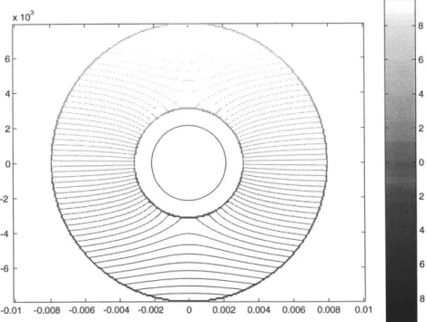
4-8 Geometry for calculating leakage reluctance path area. Three shaded blocks are the ends of the poles; we omit the rest of the sensor for clarity. 91 4-9 Contour plot of lines of constant voltage signal magnitude

|VB

secondary terminals. These are lines of constant voltage from our the-oretical analysis. We allow the center of the tube to move inside the radius r, - rt, such that we plot the voltage corresponding to the lo-cation of the center of the tube. We overlay a path of constant radius from pole one. . . . . 92

4-10 Plot of V , V, as a function of position, output from actual sensor. The signal processing board combines the three voltages from the secondary

coils into two voltages V and V. . . . .. 94

4-11 Plot of V , V, as a function of position using a first order approximation and the exact theoretical values from the Magnetic Circuit Analysis. 95

4-12 Plot of V, V, as a function of position using the adjusted values of the reluctances Rl,2t,3t. This is also a first order approximation. . . . . . 96

4-13 Plot of V , V, as a function of position using all terms. We see that the pattern is slightly closer to a perfect grid output, and that the magnitude is roughly two orders of magnitude greater. . . . . 97

4-14 Contour plot of theoretical phase of voltage VB across secondary termi-nals. We see that the phase has a different effect than the magnitude: as the tube moves in the x-direction, the phase change of VB is nearly linear in the inner area of the sensor. The units of the legend are radians. 98 4-15 Plot of V and V, using the phase of the voltages instead of the

magni-tude. The output looks even more linear than when using the magnimagni-tude. 98 4-16 Permeable, conducting, hollow cylinder in a uniform, time-varying field

imposed as the vector potential at surface (e). We assume no variation in the z direction, and finite permeability and conductivity in the tube region . . . . 100

4-17 Layout of the field problem showing the geometry we use for calculating the Fourier series representation of the field component H. . . . . 105

4-18 Magnetic field (radial-component) at surface (e) as a function of angle

0. This plot shows the complex amplitudes of the step functions. We

observe the real part of these amplitudes, so they will never all be the same at any given moment in time because of the three-phase nature of the excitation currents. . . . . 106

4-19 Derivative of radial component Hft with respect to 0 at surface (e), plotted as a function of 0. . . . . 106

4-20 Magnetic scalar potential at surface (e) at time t = 0. Here we use a

Fourier series of 51 terms to approximate the field, which we assume has discontinuous steps at the pole faces and is zero otherwise. The overshoot at the step locations is known as the Gibbs phenomenon. . 108

4-21 Magnetic field lines showing flux density inside sensor. For computa-tional reasons we only use an 11-term Fourier series approximation of the vector potential at the outer boundary as detailed above. In this case we use the actual geometry from the bench-top scale model with the 6.4 mm tube, and a 5 kHx excitation frequency. . . . . 114 4-22 Magnetic field lines showing flux density inside sensor for a tube much

smaller than the sensor opening. We impose a 11-term Fourier series vector potential at the outer surface and assume the potential in the middle is zero. The leakage flux clearly dominates. . . . . 115 5-1 Complete electronics setup. The signal generator supplies three

volt-age signals to the current sources, which power the primary coils of the sensor. The signal processing board converts the voltages from the secondary coils into two voltages V and V, which supply position information to the control computer. . . . . 118 5-2 Schematic of the three phase signal generator. The same counter drives

all three EPROMs, so that the resultant signals retain the proper phase relationships. . . . . 119 5-3 Detailed view of the output from the DAC. The two current outputs

drive the first op-amp, and the second op-amp removes the DC com-ponent of the signal. As configured, the output has a range of ±5 V . . . ... ... .. . ... . . . .. ... . . .. 123

5-4 Photograph of the top and bottom of the three-phase signal generator circuit board. We use a combination of wire wrap and solder to build the circuit. The tape strips labeled "A", "B" and "C" cover the UV window on the EPROMs so that the ambient light does not erase the memory over time. . . . . 124

5-5 Circuit diagram of the current amplifier. The inductive load is eight

primary coils from eight sensors. Three identical current supplies drive the three phases separately. . . . . 125 5-6 Current amplifier control block diagram. . . . . 129 5-7 Loop transmission of the plant and proportional controller . . . . 130 5-8 Complete transfer function from the input to the output of the current

supply . . . . 132 5-9 Demodulation circuit layout . . . . 133 5-10 Demodulation circuit wiring diagram. The top figure is the signal

layer, complete with silk screen printing which includes the text and the component outlines; the bottom figure is the power and ground layer, the thinner wires will be absorbed in the copper pour. . . . . . 137 5-11 Top view of a populated board and bottom view of a bare board.

Except for a few signal wires, the bottom of the board is exclusively for power and ground circuits. . . . . 139 6-1 Photograph of the modified E-pickup without coils or shielding, shown

with the shielding pieces. We ground the shielding at a single point to avoid closing a conductive loop around a flux path. . . . . 143

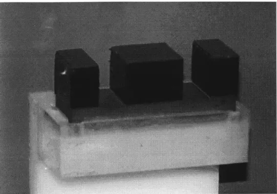
6-2 Photograph of the lamination pieces. Also shown are three sections

arranged in a circle, wrapped in Teflon tape to prevent the sharp edges from scoring the coil wire. . . . . 144

6-3 Photograph of the complete sensor, showing the coils, shielding,

lami-nations and the plastic ring which positions the components. . . . . . 146 6-4 Five sensor/actuator stations along the aluminum rail. We mount the

feet of the sensor brackets flush along one side of the rail (the right side as seen in the photograph). . . . . 147

6-5 Photograph of the sensor mount and printed circuit board. We mill

a slot out of the side of the mounting bracket for the wire to pass through. Three set-screws allow for some final positioning of the sensor as necessary. . . . . 148

7-1 Tube levitated with two sensor-actuator stations. We add magnetic

shielding to the sensor to reduce the effect of the field from the actuator on the sensor output. . . . . 150

List of Tables

2.1 Selected propertied of materials used in the construction of the sensor. 35

2.2 Summary of Maxwell's equations under the magnetoquasistatic as-sum ption. . . . . 35 2.3 Skin depth 6 as a function of frequency for selected materials. We

list the frequencies in Hertz, but convert to radians/sec for use with equation (2.29). . . . . 46

5.1 Values of components used in the demodulation circuit, as seen in Figure 5-9. . . . . 136

Chapter 1

Introduction

1.1

Overview

This thesis presents a 2-axis, noncontact position sensor for permeable steel tubes. Manufacturing processes often simultaneously require closed-loop position control and noncontact position sensing. Noncontact sensing is essential where contact might undesirably alter the surface, or where the surface is coated or contaminated in a way which makes contact problematic. Traditional electromagnetic sensors usually sense only in one direction; our design combines three one-dimensional sensors to give a two dimensional position reading with some redundant information which we use for error correction. This sensor provides the feedback device in a magnetic levitation setup using eight such sensors and eight two-axis actuators to levitate a steel tube. Along with the electromechanical design and construction of the sensor, we also present the electronic circuits which drive the sensor input and process the sensor output. These are the three-phase signal generator which commands the current supply, the current supply which drives the sensor, and the signal processing board which calculates the relevant voltages dependent on the tube position.

1.2

Background

Early in 1995, Professor David Trumper began a consulting relationship with the American Metal Handle company (AMH) to help develop a production line for metal broom and mop handles'. AMH manufactures handles in a continuous process, be-ginning with a flat strip of steel which is formed and seam-welded into a tube. The tube exits the forming mill at 1-2 meters per second, is cleaned, coated with powdered paint, heated to cure the paint, quenched in a water bath, and finally parted with a flying cutoff mechanism. From the time the paint powder is applied to the time the cured tube is quenched in water, it cannot be touched without marring the surface finish. Ten magnetic levitation stations spaced over an approximately 35 meter span levitate the metal handle during processing. Figures 1-1 and 1-2 show the actual AMH production line with the tube suspended.

Each of the ten levitation stations uses electromagnets for suspension and commer-cial eddy-current position sensors for position measurement. The suspension system is difficult to tune, but was eventually stabilized after much trial and error. While consulting for AMH, Professor Trumper realized there was a lack of general theory for noncontact sensing and actuating and submitted a proposal to the National Sci-ence Foundation; this research is conducted under funding from the resulting grant

(DMI-9700973).

The goals of the present phase of this research are three-fold: 1) design a non-contact sensor, 2) design an efficient nonnon-contact actuator, and 3) derive the control theory for stabilizing a flexible structure supported at a number of discrete locations. Doctoral candidate Ming-chih Weng and myself, along with Professor Trumper, are the principal researchers. Mr. Weng has focused on the actuator design and control system design; the sensor is the topic of this thesis. To test our results we have con-structed a -I- ₁₀ scale model using eight sensor-actuator stations to levitate a 6.4 mm steel tube. Figure 1-3 shows the bench-top scale model built in our laboratory.

Figure 1-1: Photograph of one of the quartz ovens which cure the paint on the tube. The tube diameter is approximately 22 mm. A levitation station can be seen behind the oven.

1.2.1

Sensor

We developed the sensor through a succession of design iterations. The final sensor design, shown schematically in Figure 1-4 and in a photograph in Figure 1-5, uses a differential magnetic flux measurement to determine the position of the tube, which passes through the center of the sensor. Current sources drive the three primary coils with sinusoidal currents I1, I2 and 13 at a frequency of 5 kHz. Because of the geometry

of the sensor and the magnetic permeability of the tube, the flux path depends upon the tube position. The voltages across the secondary coil terminals depend on the amount of flux linked by the coils, and thus by reading the AC voltages across the

Figure 1-2: Two levitation stations spaced approximately 3.5 meters apart stand on either side of an induction heater. The electrostatic powder paint coating station is just visible at the far right. The tube moves from right to left in this picture at a velocity of 1-2 m/sec.

secondary coils we can determine the tube position.

The primary coils drive a 5 kHz sinusoidal field which circulates through the air-gap in the center of the sensor, then back around through the laminate core. A three-phase current supply drives the sensor such that the current in each primary coil is out of phase by 120' from the neighboring primary coils. Because the poles are arranged geometrically at 120' intervals, the induced magnetic field is a 5 kHz traveling wave. A magnetic field at this frequency will only penetrate aluminum to a depth of about 1.2 mm. We design the aluminum shielding in Figure 1-4 thicker than this depth, therefore the shielding guides the flux by not allowing it to escape the air-gap region without returning through a lamination pole. Similarly, aluminum plates sandwich the sensor to reduce leakage fields in the z-direction, i.e., out of the plane of the sensor.

chang-Figure 1-3: Benchtop scale model showing five sensor and actuator pairs. We use an aluminum rail to position the components. As shown in the photo, the position of the sensor relative to the actuator alternates down the length of the setup.

ing the tube position affects the amplitude and phase of these signals. The tube position has the greatest effect on the amplitude of the signal and consequently in the present set of electronics we only use the amplitude to predict the tube position. Although this means we discard the phase information, we still use three signals to find two position measurements, which allows for error averaging.

To determine the position of the tube we use the voltages from the three secondary coils. We analyze the magnetic fields in the sensor to relate the output voltages to the tube position; inverting these relations allows us to find the tube position in terms of the output voltages. The analog circuit board shown in Figure 1-6 performs this conversion. The circuit rectifies and combines the voltage signals from the sensor and outputs two voltages proportional to the x- and y-position of the tube, respectively.

V b +

Aluminum Shielding

Primary Coil

+

Figure 1-4: Layout of the noncontact position sensor. Three current sources each drive a primary coil, which creates a flux read by the secondary coils. The flux paths, and thus the voltages induced on the secondary coils, are functions of the tube position.

1.2.2

Actuator and Controls

We use this position information and the electromagnetic actuators to levitate the tube. A Bernoulli-Euler beam model describes the tube dynamics and predicts the mode shapes and vibration frequencies. Effective placement of the actuators and sensors depends on this dynamic behavior. Placing a sensor too near a node will leave that mode unobservable, while placing an actuator there will leave the mode uncontrollable. Additionally, of necessity the actuator applies a force at a position near to, but not exactly at the position being sensed. This noncollocation means that any mode with a period smaller than twice the noncollocation distance will not be readily controllable.

In addition to the placement of the components, we must decide whether to control each station independently, or to use a state space model of the entire tube system

Figure 1-5: Photograph of the noncontact position sensor. The outer ring and inner shapes are aluminum shielding. We wrap the laminations in Teflon tape to prevent scoring the edges of the coil wire (creating a short circuit from scraping off the insu-lation); the laminations are therefore white in this photo. We pot each coil in epoxy for increased rigidity and resistance to scoring.

and control it as a whole. Doctoral candidate Ming-chih Weng is addressing this set of challenges and it is thus not the main focus of my thesis.

1.2.3

Results

Figure 1-7 is a photo of the experimental hardware, including the final design of the sensor, the signal processing circuit board, and the mounting bracket for positioning the sensor on the rail. A total of eight sensors and eight actuators form the complete setup. We fabricated an aluminum rail and sensor-actuator mounts to support and align the components. Figure 1-3 is a photo of five of these sensor-actuator pairs

Figure 1-6: Photograph of the signal processing board. The BNC output jacks connect to the control computer. We can tune the output voltages using the potentiometers on either side of the jacks.

Figure 1-7: Experimental hardware, including the sensor, the signal processing board, and the mounting hardware. The metal bracket is aluminum, and the translucent bracket is plexiglass.

mounted to the alignment rail.

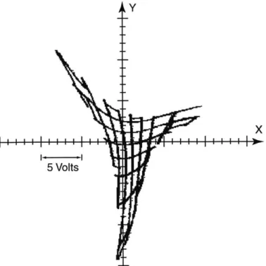
To show the linearity of the sensor output we plot the x- and y-voltages against each other as we move the tube in a grid pattern inside the sensor. To accomplish this we mount the sensor on a micrometer table with horizontal and vertical travel, (travel in the x- and y-directions respectively corresponding to the coordinate frame in Fig. 1-4). The tube is held fixed with reference to the base of the micrometer table, passing through the opening of the sensor as it would during operation. Figure 1-8 shows the path followed to give the output seen in Figure 1-9.

Y

Figure 1-8: Trace of path followed by the tube relative to the sensor which we use to estimate the linearity of the sensor output. The tube is held fixed and the sensor is moved around it so that the relative motion is as suggested by the lines in black. We then repeat this exercise for the x-direction using a similar but horizontal pattern.

Beginning with the tube in the sensor, centered in the y-direction and almost at the rightmost position in the x-direction as in Fig. 1-8, we move the sensor vertically in the negative y-direction. As the tube reaches the top of the opening we move the sensor one millimeter to the right, then vertically in the positive y-direction until reaching the lower extent of travel. We repeat this procedure until the entire inside of the sensor is covered in the y-directed lines. Repeating the same procedure for the

I-I 5 Volts

Y

X

Figure 1-9: Trace from the oscilloscope showing experimental data. The trace shows the x- and y-voltages output from the signal processing board plotted against each other as we move the tube and sensor relative to each other as shown in Figure 1-8. The ideal output is an exact trace of the path in Fig. 1-8.

x-direction gives a 1 mm grid tracing of the opening.

During this tracing procedure the oscilloscope records x- and y-voltages from the signal processing board; we call these V and V, respectively. Using two inputs to the scope allows us to plot the data in x vs. y format (as opposed to the default x vs. time format). The "infinite persistence" setting on the scope keeps the entire trace history on the screen. We save this data trace and export it to a file. This is the plot shown in Figure 1-9.

The deviation from linearity is obvious in the output. If the output were perfectly linear the plot would resemble a perfect grid truncated by the circular shape of the sensor opening, i.e., the path traced by the tube. When the tube is near the center of the sensor, the grid shape is clearly visible. However, as the tube nears the edges of the sensor aperture, and especially as it nears the poles, the deviation from linearity increases. The three "points" seen in the experimental output are a result of the increased sensitivity as the tube nears one of the three poles. In these areas, 1 mm of

movement results in a larger change in the output voltage than that corresponding to 1 mm of movement in the center of the sensor. For use with the control system we adjust the output gain on the signal processing board so that 2 mm of displacement on either side of center spans the output voltage range of ± 10 V.

1.3

Thesis Layout

This chapter outlines the goals of the research, the topics covered in this thesis, and gives a brief description of the final sensor design. We organize the rest of the thesis as follows. Chapter 2 presents a background in the necessary theory to familiarize the reader with the concepts used in the rest of the analysis. We present relevant sensor operation principles and topologies in Chapter 3. In Chapter 3 we also describe the

design evolution of the sensor. Chapter 4 develops the mathematical analysis of the sensor's operation and compares this to the experimental results. This comparison also helps to refine the parameters used in the analysis. Chapter 5 presents the design and construction of the electronic circuits necessary for driving the sensor and processing its output waveforms, including the signal generator board, current supply, and the signal processing board. Chapter 6 presents the sensor construction, including material choice and machining. Chapter 7 summarizes the results presented in this thesis and discusses possibilities for future work.

Chapter 2

Background Theory

In this chapter we establish the theory used to analyze the electromagnetic systems developed in this thesis. Maxwell's equations, as simplified by the magnetoquasistatic assumption, form the basis of the analysis from which we explore effects such as skin depth and magnetic diffusion. We develop a lumped parameter revision of these equa-tions via the Magnetic Circuit Analogy (MCA), which is useful where the geometry of the problem is complex and we prefer to work with lumped reluctances [10].

Because many references discuss Maxwell's equations, only a brief introduction follows in this thesis. We encourage the interested reader to investigate [2, 7] and [16] for a more thorough discussion. We first demonstrate the usage of these equations in magnetic circuits by way of a simple example problem, i.e., the air-gap transformer seen in Figure 2-1. When the geometry of the problem does not facilitate the direct solution of Maxwell's equations, we can frequently take a lumped-parameter approach for simplification. We introduce one such lumped parameter method, the MCA, in the context of the example problem in order to compare the two methods.

When the system involves conducting materials, alternating magnetic fields give rise to alternating currents, which in turn affect the field distribution. We present these magnetic diffusion effects as well; specifically with respect to shielding, skin depth and the issue of what we can consider "perfect" conduction.

2.1

Notation

Many of the variables in this analysis are sinusoidal signals which we represent using complex exponential notation as described in

[7].

<D (x, y, z, t) = Re{(x, y, z)ewt}, (2.1)

where 1(x, y, z) is the complex amplitude of the signal. Similarly, when we use a variable in polar coordinates which has a complex amplitude that varies sinusoidally with 0 and time, we use

<D(r, 0, z, t) = Re{<i(r, z)e(Wtmo)}. (2.2)

The variable m is the angular wave number, and assumes only integer values.

2.2

Maxwell's Magneto quasistat ic Equations

2.2.1

MQS Assumption

Maxwell's equations summarize the rules electromagnetic fields have been found to obey. Depending on the system parameters we may make some simplifications; the most helpful in this situation is the magnetoquasistatic (MQS) assumption. We will consider a system MQS if the characteristic time of interest (here, the reciprocal of the excitation frequency) is much larger than the time it takes an electromagnetic wave to propagate over a characteristic length. Dividing the characteristic length by the speed of light and comparing to the characteristic time, the equation

L << r

(2.3)

C

holds for MQS systems. Here, c is the speed of light in a vacuum, T is the reciprocal

length. We use L = .075 m, the largest dimension in the system.

these numbers gives

Substituting in

.075m

3x 2.5 x 10-1 <<2.0 x 10 4sec. (2.4)

Therefore we may analyze this system using MQS techniques.

Also, we assume the materials we use to construct the sensor are magnetically

linear, such that B = pH and p is constant. Table 2.1 shows typical values for

the permeability y and the conductivity - of the materials we use for the sensor construction.

Material Conductivity (-,200 C) Permeability (j)

Aluminum 3.54 x 107 47r x 10-7 = pL

Steel Tube 0.75 x 107 ~ 5 x 103Po

Silicon Iron Lamination 2.1 x 106 ~ 7 x 10'p1

Table 2.1: Selected propertied of materials used in the construction of the sensor.

To summarize the MQS versions of Maxwell's equations we present Table 2.2.

Integral Form Differential Form Boundary Condition

Ampere fcHds fs J da V x H= J n x [H]=K

f dt __ ___________

Faraday

#cE

IsZ-da

Gaussf B - da=0 V -B =0 n- [B] =0

Table 2.2: Summary of Maxwell's equations under the magnetoquasistatic assump-tion.

2.2.2

Example Problem

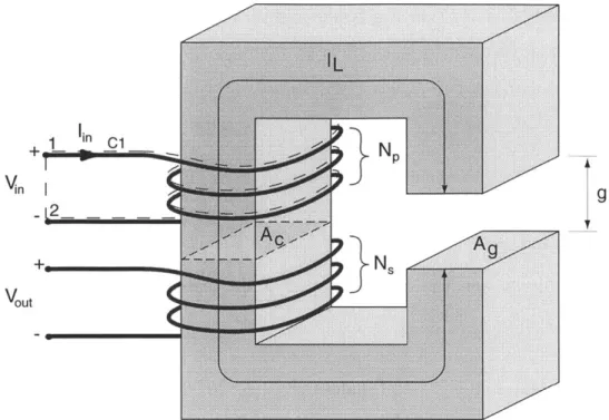
We analyze an example problem to compare the direct application of Maxwell's equa-tions to a solution using the Magnetic Circuit Analysis. Figure 2-1 shows a permeable core transformer with a small air gap. A voltage Vi drives the primary coil causing

1 in Cl_

V

ouA

Figure 2-1: Example magnetic circuit. A voltage Vm. across the primary coil drives a flux which links the secondary coil. We assume the air gap is small enough that we may ignore the fringing of the field.

a current Ii*n to flow through the coil. This current induces a magnetic field Hc in the core and magnetic field Hg in the air gap. We ignore the fringing fields by assuming that the gap g is much smaller than either dimension of the cross-sectional area Ag. For simplicity we assume the cross-sectional area of the air gap is the same as the cross-sectional area of the core, i.e., Ac Ag. If this were not so, the change in flux

density as a function of position along path 1_{L would be inversely proportional to the} change in area, as BA remains constant along the path 1

L

+

(because

Ag and Ac through the calculations as distinct parameters to clearly distinguish to

which area we refer.

Ampere's Law

HlL + Hgg =NIn. (2.5) Since we model the secondary coil as an open circuit, no current flows in this wire.

If there were a current in the secondary coil, it would show up on the left side of

equation (2.5) as an additional term NIs.

Gauss' Law (Magnetic)

Gauss' law specifies that the net flux passing through a closed surface is zero. We select a surface which encloses only the top half of the core and passes through the air gap, and use the constitutive law for linear magnetic materials to give

oHgAg = pHeAc. (2.6)

Faraday's Law

Faraday's law relates the electric field along a closed contour to the flux passing through the contour. In this case the contour is C1, which goes from point 2 to point

1 across the voltage Vn, then through the coil back to point 2. We can break up the

total integral into the integral across the terminals plus the integral along the wire. Employing Ohm's law for conductive materials (J = u) in the wire gives

j E-dl= E-dl+ 121-dl. (2.7)

terminals coil

The electric field across the terminals is simply the voltage Vin divided by the distance separating the terminals, so integrating from 2 to 1 returns -Vin. Along the wire, the current density J is the current Iin divided by the cross-sectional area of the wire, A.c. Integrating along the length of the wire returns IinR, where we define R as

R = 'w'' (2.8)

o-Axec

i1 E -dl = -Vin + I2nR. (2.9) The right side of Faraday's equation concerns the magnetic flux density linked by the coils. We assume the flux is constant across the area and parallel to the surface normal n'. As a result, the dot product in the integral returns the magnitude of the magnetic flux, which we denote simply as B. The result of the integral is thus the product BAcN,, where N, is the number of turns of the primary coil. Therefore

d d

B -n dA= - (BAcNp),7 (2.10)

dt A dt

and the result of applying Faraday's law is

dB

Vin - IinR = AcNp .B (2.11)

dt

Recall that the cross-sectional areas of the air gap and coil are the same; this means the magnetic flux density B is constant throughout the magnetic circuit.

To find the voltage V0st across the secondary coil we again use Faraday's law, but this time the terminals are an open circuit so that the current is zero. Assuming the flux density B is constant over the cross sectional area of the laminations (and perpendicular as above) Faraday's law reduces to

Vout = NAc dB (2.12)

dt

2.2.3

Transfer Functions

We may now write two important transfer functions using the above relationships. Solving equation (2.6) for He and substituting into (2.5) gives

NpIin = Hg (g + "~ . (2.13)

We now combine this with (2.12). Replacing the time derivative with the Laplace variable s to simplify the equations results in the transfer function

I-- s _{._ (2.14)}

in g +

Solving (2.11) for Vi and substituting equation (2.13) gives an equation for X, in terms of H.,

VUn= Hg s(tptNAc ) + R (g + pogL .(2.15)

N, pAc

Dividing equation (2.12) by (2.15) and using B = poHg results in the transfer function from Vin to Vut,

Vout s(poNpNsA) (2.16)

Kn _{s(upoNpAc) + R (g +}

An important point is immediately evident: using a current source for 'in (2.14) instead of a voltage source for Vn (2.16) results in a much simpler transfer function.

Because the volumes and areas involved here are rather basic, we can easily compute the integrals in Maxwell's equations. Sometimes the geometry is more complex. In this case we can adopt the Magnet Circuit Analogy formulation to allow us to write the equations in a more direct manner.

2.3

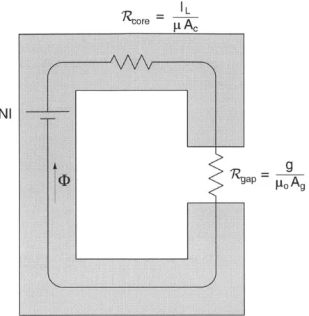
Magnetic Circuit Analogy

In the preceeding analysis we assumed that the quantities g and Ag were known and constant. Often in magnetic circuits, the exact path of the flux (defined by g and Ag) is unknown, and is a function of the position of some part of the circuit (as in an electromagnetic actuator where the flux travels through the moving target).

Combining the unknowns g and Ag with the permeability p into a single unknown quantity can simplify the analysis. We define the reluctance R as:

R=

g

pgAg

loop is equal to the current density passing through the surface area bounded by the loop. When the flux density B is constant over an area A, we can simplify the flux

<D to the product BA, where we define the surface area normal vector n' parallel to

the direction of the magnetic flux so that the vector dot product B - n returns the magnitude B. Also, we use the relation B = pgH and rewrite Ampere's law as

g A ds =J - da = J Ax. (2.18)

Here we assume the current density is perpendicular to the cross-sectional area of the wire, giving the same simplification described above. The product JA.c equals the total current; if the wire carries current i and is arranged as a coil with N turns we can also express this as Ni.

For the MCA, we define sections of flux path as reluctances, and assume that the quantities pg, A are constant in each section; this allows us to pull them out of the integral above. When a connected path of n such reluctances encircles a total current density of Ni, we can write equation (2.18) as a sum of these reluctances,

E <DjRj = Ni. (2.19)

j=1

In the magnetic circuit analogy we treat the current density Ni (or magnetomotive

force) as a voltage, the reluctance as a resistance, and the flux as a current. The above

equation (2.19) is thus analogous to Kirchoff's Voltage Law. Similarly, Gauss' law supplies the analogous equation for Kirchoff's Current Law, by requiring that the net flux (current) entering a closed surface (node) be zero. Equipped with these new relations we model the above magnetic circuit by overlaying the components with their MCA equivalents, as indicated in Figure 2-2.

The proper choice of g and Ag is important for the accuracy of the solution; choosing these assumes detailed knowledge of the flux paths. Across small air gaps, the choice is obvious; but for large gaps and non-uniform geometry we must guess

g and Ag. We can describe the system in terms of known inputs Ni and unknown

Rre L A

A,

..0 ... ....

NI

ap g

Figure 2-2: Magnetic circuit element representation of the example problem. The resistive and voltage source elements model the behavior of the sensor, allowing us to solve for the terminal relations using traditional circuit analysis methods.

more accurate the model. The rules for addition of reluctances in series and in parallel directly follow those for resistances in the traditional circuit.

To find the flux, we solve the circuit of Figure 2-2 using standard circuit analysis methods with the reluctances as shown in the figure. As before we assume the fringing of the field across the air gap to be negligible. Applying Kirchoff's Voltage Law to the loop in Figure 2-2 gives

NI

+L pog

(2.20)

The secondary coil, of inner area Ac and N, turns, encircles this flux, resulting in V,, across the terminals. Applying Faraday's law results in

Vout - (Nsb), (2.21) dt

where the terminals are still an open circuit so the current in the wire is zero. Solving for the relevant transfer function,

Vout NpNs poNpNsAg(

+=i~ 1 g+ h~

s__=_s _(2.22)

I- -T,-+ g g+ pogl

In Ac po,,A9 9 pAc

which is the same as we found using the integral forms of Maxwell's equations. The main simplification is the lumping of the geometric parameters into a single reluctance term. The validity of the answer still depends on our choice for these reluctances, but these are now simple lumped parameters rather than areas of integration. Most importantly, we may use traditional circuit analysis rules to derive the system rela-tions.

2.4

Magnetic Diffusion Equation

A time-varying magnetic field can induce an electric field in a conductor; this

interac-tion is called magnetic diffusion. Like Maxwell's equainterac-tions in the previous secinterac-tion, we limit this derivation to the extent relevant to our application. For a more complete analysis, we direct the reader to [16, 2] and [7].

For the derivation of the magnetic diffusion equation, the differential form of Maxwell's equations are most convenient. The first step is to combine Ampere's law with the constitutive law for Ohmic materials,1

V x H = f = UE. (2.23)

We take the curl of both sides, and substitute Faraday's law in for V x E, giving

OpN

V x V x H = - . (2.24)

Finally, a vector identity 2 reduces the magnetic diffusion equation to it's most familiar

form,

V2H =o-p (2.25)

at

The magnetic field inside a conductor will satisfy this equation.

2.4.1

Skin Depth

To predict whether the flux will be repelled from the tube or attracted to it, we examine the rules of magnetic diffusion. Because of the effect described by Ampere's law, an imposed field can induce a volume current in the conductor which will tend to repel the original field. The field decays exponentially with depth into the conductor. The depth to which the field penetrates a conductor, known as the skin depth, depends on the frequency of excitation and the material properties of the conductor. For the ideal "perfect conductor" with infinite conductivity and with permeability yuo, the field is completely repelled; while for an insulator with zero conductivity and permeability PO, the field will pass straight through. For this analysis we assume the surrounding medium is air, which is nonconducting and has permeability po.

This derivation loosely follows those presented in [15] pp. 442-443 and [16] pp.

358-360. The field inside a conductor must satisfy (2.25). Assuming an x-directed,

sinu-soidally varying magnetic field is imposed tangentially upon a conductor as shown in Figure 2-3, we propose the resulting field inside the conductor will take the general form

Hx(y, t) = Re{Hx(y)ejwt}. (2.26)

Substituting this into (2.25) gives

d2H(

dy"= jo-pwH2. (2.27)

2

Lo

air

y

H

x

z

Figure 2-3: Field H, incident upon a conductor. Because of the conductivity, an opposing field is created in the conductor to repel the original field, thus limiting the penetration of the imposed field into the conductor.

Here we use the fact that H, only varies spatially with y to simplify the Laplacian in (2.25). Substituting a general solution of the form H5(y) = Aie(a+j)y + A2e(a-b)Y

into the above equation and cancelling like terms gives

(a i jb)2 _{= jPWo-, (2.28)}

which we simplify by defining the skin depth 6 as

r 2

AL=J (2.29)

Using the relation 0j = !+! and solving equation (2.28) for a ± jb in terms of 6 results in a solution of the form

(1+j)y -- (1+)

H5(y) = Aie 6 + A2e 6 , (2.30)

where A1 and A2 are constants determined by the boundary conditions. In this case, we may set A1 to zero because we assume the field decays as depth y increases. The total field is now a product of exponentials, and rearranging them makes the behavior of the magnetic diffusion wave more obvious:

Re{A2 e j(wt)}. (2.31)

The wave is a product of one exponential which decays at a rate j and another which oscillates at a frequency w at a fixed location, and travels with phase velocity y = 6w.

0I 0.8 0.6 0.4 0.2 0.2 0 1 2 3 4 5 6 y/6

Figure 2-4: Skin depth of a magnetic field in a conductor. On the j 0 edge, the

induced field inside the conductor instantaneously equals the applied H field. The imposed field varies sinusoidally with time; the field in the conductor is a traveling wave.

In a lumped parameter analysis the skin depth is a fixed quantity; the magnetic field in a conductor is assumed constant to a depth 6 and zero afterwards. This differs from the exact solution detailed above, which is a diffusion wave. Figure 2-4 shows the lumped parameter estimation for the skin depth, along with the diffusion wave at four different moments in time. We obtain these curves by varying the time t and keeping the frequency w constant, such that the product wt takes on the values 0,, !1 and 1._{'4 3 2} The horizontal axis in the figure is the distance into the conductor, normalized to 6; the vertical axis is the x-component of the magnetic field, normalized to the incident

field magnitude H,,. These normalizations follow naturally from the derivation above when we recognize that the boundary condition described by Ampere's Law forces the constant A2 in equation (2.31) to equal the incident field magnitude. This is because we model the conductor as having volume currents but not surface currents. As seen in (2.31), even at time t = 0 when the product wt is zero, (assuming steady-state conditions exist), the field still varies as an exponentially decreasing sinusoid in the conductor.

In Table 2.3 we calculate the lumped parameter skin depths for the three main materials used in the sensor for three different frequencies, using (2.29).

f

f

f

f

Silicon-Iron 0.0417 mm 0.035 mm 0.0132 mm 0.00417 mm

Steel 0.0784 mm 0.0186 mm 0.0248 mm 0.00784 mm

Table 2.3: Skin depth 6 as a function of frequency for selected materials. We list the frequencies in Hertz, but convert to radians/sec for use with equation (2.29).

2.4.2

Attraction or Repulsion

As a general rule for a conductor with permeability close to yA, whenever the thickness of the material is greater than the skin depth we model it as a perfect conductor, which will repel an imposed field. The field inside a real conductor decays as frequency increases but is never zero throughout, even inside a superconductor [16] pp. 450-451. However, we may safely approximate it as zero if it is much smaller in magnitude than other fields of concern in the system; in this case we say the conductor repels the field. For the steel tube we use in our setup, the skin depth at 5 kHz is 6 = 0.0186

mm and the wall thickness is 1 mm, implying that the field in the tube would be negligible if the steel were non-permeable. However the permeability of the steel is much higher than py, and experimental evidence shows the field is still attracted to the tube at 5 kHz. We confirm this experimentally since as we move the tube towards