HAL Id: hal-00296212
https://hal.archives-ouvertes.fr/hal-00296212
Submitted on 3 May 2007
HAL is a multi-disciplinary open access
archive for the deposit and dissemination of
sci-entific research documents, whether they are
pub-lished or not. The documents may come from
teaching and research institutions in France or
abroad, or from public or private research centers.
L’archive ouverte pluridisciplinaire HAL, est
destinée au dépôt et à la diffusion de documents
scientifiques de niveau recherche, publiés ou non,
émanant des établissements d’enseignement et de
recherche français ou étrangers, des laboratoires
publics ou privés.
campaigns
J. D. Fast, B. de Foy, F. Acevedo Rosas, E. Caetano, G. Carmichael, L.
Emmons, D. Mckenna, M. Mena, W. Skamarock, X. Tie, et al.
To cite this version:
J. D. Fast, B. de Foy, F. Acevedo Rosas, E. Caetano, G. Carmichael, et al.. A meteorological overview
of the MILAGRO field campaigns. Atmospheric Chemistry and Physics, European Geosciences Union,
2007, 7 (9), pp.2233-2257. �hal-00296212�
www.atmos-chem-phys.net/7/2233/2007/ © Author(s) 2007. This work is licensed under a Creative Commons License.
Chemistry
and Physics
A meteorological overview of the MILAGRO field campaigns
J. D. Fast1, B. de Foy2,*, F. Acevedo Rosas3, E. Caetano4, G. Carmichael5, L. Emmons6, D. McKenna6, M. Mena5, W. Skamarock6, X. Tie6, R. L. Coulter7, J. C. Barnard1, C. Wiedinmyer6, and S. Madronich6
1Pacific Northwest National Laboratory, Richland, WA, USA
2Molina Center for Energy and the Environment, La Jolla, CA, USA
3Comisi´on Nacional del Agua, USMN-GRGC, Boca del R´ıo, Veracruz, M´exico
4Centro de Ciencias de la Atm´osfera, Universidad Nacional Aut´onoma de M´exico, M´exico City, M´exico
5University of Iowa, Iowa City, IA, USA
6National Center for Atmospheric Research, Boulder, CO, USA
7Argonne National Laboratory, Argonne, IL, USA
*now at: Saint Louis University, Saint Louis, MO, USA
Received: 11 December 2006 – Published in Atmos. Chem. Phys. Discuss.: 13 February 2007 Revised: 17 April 2007 – Accepted: 19 April 2007 – Published: 3 May 2007
Abstract. We describe the large-scale meteorological
condi-tions that affected atmospheric chemistry over Mexico dur-ing March 2006 when several field campaigns were con-ducted in the region. In-situ and remote-sensing instrumenta-tion was deployed to obtain measurements of wind, temper-ature, and humidity profiles in the boundary layer and free atmosphere at four primary sampling sites in central Mex-ico. Several models were run operationally during the field campaign to provide forecasts of the local, regional, and syn-optic meteorology as well as the predicted location of the Mexico City pollutant plume for aircraft flight planning pur-poses. Field campaign measurements and large-scale anal-yses are used to define three regimes that characterize the overall meteorological conditions: the first regime prior to 14 March, the second regime between 14 and 23 March, and the third regime after 23 March. Mostly sunny and dry con-ditions with periods of cirrus and marine stratus along the coast occurred during the first regime. The beginning of the second regime was characterized by a sharp increase in hu-midity over the central plateau and the development of late afternoon convection associated with the passage of a weak cold surge on 14 March. Over the next several days, the at-mosphere over the central plateau became drier so that deep convection gradually diminished. The third regime began with the passage of a strong cold surge that lead to humid-ity, afternoon convection, and precipitation over the central plateau that was higher than during the second regime. The frequency and intensity of fires, as determined by satellite
Correspondence to: J. D. Fast
measurements, also diminished significantly after the third cold surge. The synoptic-scale flow patterns that govern the transport of pollutants in the region are described and com-pared to previous March periods to put the transport into a climatological context. The complex terrain surrounding Mexico City produces local and regional circulations that govern short-range transport; however, the mean synoptic conditions modulate the thermally-driven circulations and on several days the near-surface flow is coupled to the ambient winds aloft.
1 Introduction
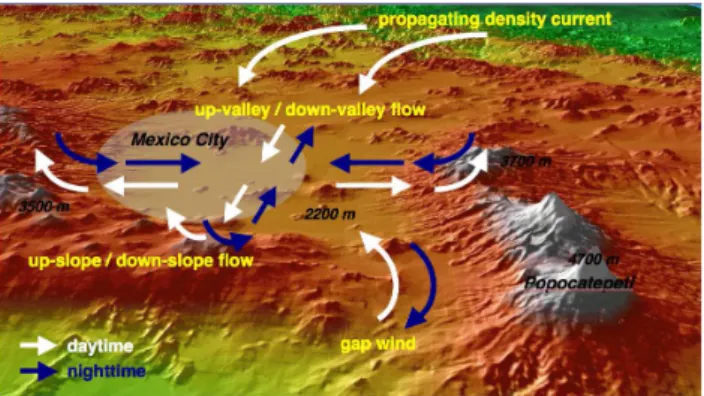
The rapid growth of megacities has led to serious urban air pollution problems in many developing countries. For ex-ample, Mexico City is the largest metropolitan area in North America with a population of ∼20 million. In addition to the sources of trace gases and aerosols resulting from human activities, the local meteorological conditions influenced by the surrounding terrain strongly affect the poor air quality that is observed. As shown in Fig. 1, Mexico City is lo-cated within a basin on the central Mexican plateau at an elevation of ∼2200 m above sea level (m.s.l.) at ∼19.4 N latitude. Mountain ranges that are ∼1000 m higher than the basin floor border the west, south, and east sides of the city. The mountain ranges include several tall peaks, the tallest being the Popocatepetl volcano located southeast of Mexico City with an elevation of 5465 m m.s.l. The gap in the moun-tains at the southeast end of the basin also affects the local
Fig. 1. Schematic diagram depicting types of thermally-driven flows that have been observed in the vicinity of Mexico City. White and blue arrows denote daytime and nighttime wind directions, re-spectively. Topography elevation (m) at select locations denoted by black text.
basin circulations (Doran and Zhong, 2000; Jazcilevich et al., 2003; de Foy et al., 2006a).
The generally light synoptic winds, subtropical and high-altitude insolation, formation of shallow stable boundary lay-ers at night, and boundary-layer circulations influenced by the complex terrain (J´auregui, 1988; Lauer and Klaus, 1975) combine to produce frequent episodes with elevated levels of ozone and particulate matter during the entire year (Collins and Scott, 1993; Garfias and Gonzolas, 1992; Raga et al., 2001). The thermal and dynamic effects of urbanization also modify boundary layer properties (J´auregui, 1997; Oke et al., 1999) and subsequently near-surface transport and mixing of pollutants. In addition to anthropogenic sources, partic-ulate concentrations are influenced by dust (Edgerton et al., 1999; Vega et al., 2002) and sulfate produced downwind of Popocatepetl (Raga et al., 1999b) and the Tula refinery com-plex (Johnson et al., 2006). Measurements of cloud conden-sation nuclei (CCN) concentrations are linked to particulate concentrations in Mexico City (Baumgardner et al., 2004), suggesting that anthropogenic sources may alter local pre-cipitation (J´auregui and Romales, 1996).
As a result of several recent field campaigns, much is known about the boundary layer evolution and transport pro-cesses in the immediate vicinity of Mexico City that affect trace gases and aerosols. Meteorological and chemical mea-surements made over the southern mountain range during the 1997 Azteca experiment indicated that up-slope flows trans-ported pollutants out of the city to higher elevations dur-ing the day, and down-slope flows transported a portion of the pollutants back towards the city at night (Raga et al., 1999a; Baumgardner et al., 2000). A mesoscale model pre-dicted the development of a propagating density current dur-ing the 1991 Mexico City Air Quality Research Initiative (MARI) resulting from the horizontal temperature gradient between the warmer basin atmosphere and cooler marine air east of the Sierra Madre Oriental along the Gulf of Mexico (Bossert, 1997); however, there were relatively few
measure-ments to provide direct observational evidence of the circula-tion. Measurements from four meteorological profiling sites consisting of radar wind profilers and radiosondes during the 1997 Investigacion sobre Materia Particulada y Deteri-oro Atmosferico-Aerosol and Visibility Research (IMADA-AVER) field campaign (Doran et al., 1998; Edgerton et al., 1999) showed that propagating density currents frequently produced strong near-surface northerly flows, lower temper-atures, and higher humidity over the northern basin. Based on the meteorological profiles, Whiteman et al. (2000) found the boundary layer evolution and regional flows were deter-mined primarily by the plateau topography; however, some-what more heating and cooling in Mexico City resulted from the basin topography. Strong southeasterly flow in the form of a low-level jet through the terrain gap in the southeastern corner of the basin was observed to develop frequently dur-ing IMADA-AVER as a result of the horizontal temperature gradient between the warmer basin atmosphere and cooler free atmosphere to the south (Doran and Zhong, 2000). Sur-face wind measurements over the city indicated that the op-posing propagating density current and gap flow produces strong convergence in the basin during the late afternoon. Routine and special measurements made during the 2003 Mexico City Metropolitan Area (MCMA-2003) field cam-paign showed that the location of the largest ozone concen-trations in the city depended on the interaction of the syn-optic conditions and local thermally-driven flows (de Foy et al., 2005). Downward momentum flux was also found to in-fluence the evolution of the convergence zone (de Foy et al., 2006a). Dispersion modeling studies (Fast and Zhong, 1998; de Foy et al., 2006b; Jazcilevich et al., 2005) have shown that the near-surface convergence and other thermally-driven flows can effectively ventilate pollutants out of the basin and reduce the likelihood of multi-day accumulation of pollu-tants. A schematic diagram depicting the various thermally-driven flows that have been observed in the vicinity of Mex-ico City is shown in Fig. 1.
Conversely, there have been very few meteorological and chemical measurements in the surrounding region that can be used to describe the fate of pollutants originating from Mex-ico City. In addition to affecting regional air quality, aerosols originating from Mexico City may also impact the local and regional climate by altering the radiation budget (Jauegui and Luyando, 1999; Raga et al., 2001). To better understand the evolution of trace gases and particulates originating from an-thropogenic emissions in Mexico City and their impact on regional air quality and climate, a field campaign called the Megacities Initiative: Local And Global Research Observa-tions (MILAGRO) collected a wide range of meteorological, chemical, and particulate measurements during March 2006. Measurements were also obtained over a wide range of spa-tial scales from local, regional, and large-scale field experi-ments to describe the evolution of the Mexico City pollutant plume from its source and up to several hundred kilometers downwind.
1 181 361 540 720 900 1 181 361 540 720 900(a) Acapulco Veracruz Mexico City Gulf of Mexico Pacific Ocean Sierra Madre del Sur Sierra Madre Oriental Gulf of Tehuantepec 412 429 446 463 480 497 385 402 419 436 453 470(b) T0 T1 T2 Santa Ana Popocatepetl Tula Toluca Cuernavaca Pachuca Puebla 412 429 446 463 480 497 385 402 419 436 453 470(c) T0 T1 T2
Fig. 2. Locations of various measurement sites during the MILAGRO field campaigns including (a) operational rawinsonde (red dots) and
surface meteorological sites (light blue dots) over Mexico, (b) operational surface meteorological sites (light blue dots), operational air quality and meteorology sites (dark blue dots), MILAGRO super-sites (yellow dots), and other MILAGRO sites (green) in the vicinity of Mexico City, and (c) typical aircraft flight paths over the surface sampling sites by the G-1 aircraft during the morning (blue) and afternoon (red). Light red shading denotes urban areas and gray shading denotes topography, with contour intervals of 200 m in (b) and (c).
MILAGRO was composed of five collaborative field ex-periments. The MCMA-2006 field experiment, supported by various Mexican institutions and the U.S. National Sci-ence Foundation (NSF) and Department of Energy (DOE), obtained measurements at several surface sites over the city. Measurements in the city and regional measurements up to a hundred kilometers downwind of the city were obtained from the G-1 and B200 aircraft during the Megacities Aerosol Ex-periment (MAX-Mex) supported by the DOE. The Megaci-ties Impact on Regional and Global Environments – Mexico (MIRAGE-Mex) field experiment, supported by the NSF and Mexican agengies, obtained regional and large-scale mea-surements up to several hundred kilometers downwind of Mexico City using the C-130 aircraft. Large-scale measure-ments downwind of Mexico City as far as the northern Gulf of Mexico were collected by the DC-8 and J31 aircraft dur-ing the Intercontinental Transport Experiment B (INTEX-B), supported by the National Aeronautical and Space Adminis-tration (NASA). Finally, a Twin Otter aircraft was used to sample biomass burning smoke plumes in central Mexico, with support from the USDA Forest Service and the NSF.
In this study we describe the rationale for the meteo-rological sampling strategy that was developed for MILA-GRO, the forecasting activities that supported the research aircraft sampling, and the synoptic meteorological condi-tions observed during the field campaign. Large-scale me-teorological analyses, routine surface and satellite data, and MILAGRO meteorological measurements are employed to describe the synoptic conditions influencing the transport, transformation, and fate of atmospheric trace gases and aerosols downwind of Mexico City.
2 Meteorological sampling
Operational meteorological measurements in Mexico are rel-atively sparse compared to the U.S. Figure 2a shows the lo-cations of the rawinsondes that obtain vertical profiles of pressure, temperature, humidity, and winds and shows the locations of surface meteorological stations operated by the Servicio Meteorol´ogico Nacional (SMN). Rawinsondes are launched twice per day from Mexico City at 00:00 and 12:00 UTC, but only once per day at 00:00 UTC at the
re-maining sites. These soundings are assimilated into
Na-tional Center for Environmental Prediction (NCEP) opera-tional models to produce synoptic-scale analyses that are also the initial conditions for multi-day forecasts. Since most soundings are made only once per day, the synoptic-scale analyses at 06:00, 12:00, and 18:00 UTC may contain larger uncertainties over Mexico than at 00:00 UTC. Therefore, the rawinsonde network was supplemented so that soundings were made four times per day at 00:00, 06:00, 12:00 and 18:00 UTC at Mexico City, Veracruz, and Acapulco. The goal was to improve the synoptic-scale analyses in the re-gion so that operational NCEP and MILAGRO model fore-casts (described in Sect. 3) would be more accurate.
The month of March was selected for the field campaign period because of the dry, mostly sunny conditions observed over Mexico at this time of the year (J´auregui, 2000). Clouds and precipitation that would complicate aircraft sampling and scavenge a portion of the pollutants in the region usu-ally increase during April. To achieve the scientific goals of MILAGRO, the surface sampling sites needed to be lo-cated on the central plateau within a hundred kilometers of Mexico City. Farther downwind along the coast, the pollu-tant plume would likely become decoupled from the marine
boundary layer and surface instrumentation located in that region would likely sample pollutants primarily from local sources. The aircraft flight tracks also needed to pass over the surface sites so that Mexico City pollutant plume could be sampled both at the surface and at multiple altitudes at the same time.
Therefore, the MILAGRO modeling working group con-ducted a series of studies prior to the field campaign to de-termine the primary regional and long-range transport path-ways downwind of Mexico City, to help select the loca-tion of surface sampling sites, and to design aircraft sam-pling flight tracks. These studies used trajectories computed from historical synoptic-scale analyses and the HYSPLIT model (Draxler and Rolph, 2003) for February and March of 2002 and 2003, additional analysis of dispersion simu-lations described in Fast and Zhong (1998) and de Foy et al. (2006b) for February–March 1997 and April 2003, and regional chemistry simulations for select multi-day periods for meteorological conditions in March 1997 and 2005. The results suggested that the Mexico City pollutant plume is transported northeastward 20–30% of the time during March. There was no preferred direction for the remaining time dur-ing March.
The principal surface sampling sites in the vicinity of Mexico City selected by MILAGRO scientists are shown in Fig. 2b. The T0 site, located in the northwestern part of the basin, was selected to measure fresh pollutants representa-tive of the Mexico City metropolitan area. The T1 site, lo-cated just north of the basin, was selected to measure a mix-ture of fresh and aged pollutants as they exit the metropoli-tan area. The T2 site, located about 35 km northeast of T1, was selected to measure aged pollutants as they are trans-ported from Mexico City towards the northeast into the re-gional environment. The site names were derived from the sampling strategy to measure polluted air over the city and then at two times downwind during periods of southwest-erly flow. An example of G-1 aircraft flight tracks is shown in Fig. 2c that depicts sampling aloft over the three princi-pal sites and across the Mexico City pollutant plume during transport towards the northeast. The B200 and C-130 aircraft also frequently sampled over the surface measurements sites. Figure 2b also shows the location of the routine air quality monitoring sites as well as special meteorological, chemi-cal, and particulate measurement sites deployed as part of the MCMA-2006 experiment and experiments lead by sci-entists from the Universidad Nacional Aut´onoma de M´exico (UNAM) and Insituto Mexicano del Petr´oleo (IMP) scien-tists.
In addition to the wide range of chemical and particu-late instrumentation, meteorological instrumentation was de-ployed at T0, T1, and T2 to measure the evolution of wind fields and boundary layer properties that affect the vertical mixing, transport, and transformation of pollutants. Radar wind profilers at each site obtained wind speed and direc-tion profiles up to 4 km a.g.l. at half hour intervals. A radar
wind profiler was also deployed at Veracruz, located on the Gulf of Mexico east of Mexico City to obtain wind infor-mation aloft farther downwind of Mexico City. The wind profiles obtained at Veracruz extended as much as 1.5 km above the elevation of the central Mexican plateau. Several radiosondes were launched from T1 and T2 on G-1 research aircraft sampling days to obtain temperature and humidity profiles that characterize boundary layer growth and once per day on days when there were no G-1 flights. Some of these radiosondes also obtained wind profiles that extended above the radar wind profilers measurements. Temperature and humidity profiles at T0 were obtained at 1-min intervals up to 10 km a.g.l. from a microwave radiometer (Karan and Knupp, 2006). A micro-pulse lidar (Campbell et al., 2002) and tethersondes were also deployed at T0 and T1 to obtain additional information on boundary layer properties.
3 Operational forecasting
A team of modelers produced daily weather briefings during the field campaign that consisted of current and forecasted meteorological conditions as well as the likely location of the Mexico City pollutant plume. These briefings, presented to scientists located at the Veracruz center of operations, were designed to contain information needed to plan and coor-dinate aircraft flight plans several days in advance. While NASA’s DC-8 aircraft was deployed at Houston, the other five research aircraft were based at Veracruz. Veracruz’s sea-level location permitted larger instrument payloads than would be possible at airports located on the plateau. Con-sequently, a large fraction of the aircraft operation scientists were located in Veracruz.
In addition to operational meteorological information such as satellite images and NCEP model forecasts products, the modeling team relied on real-time data from the radar wind profiler network and the micro-pulse lidar at T1 for current information on the winds and boundary layer depth over the central plateau. Several research models, listed in Table 1, were run during the field campaign to forecast the position of the Mexico City pollutant plume as well as regional and syn-optic variations in the distribution of trace gases and aerosols. Individual models produced a combination of meteorology, dispersion, chemistry, or particulate forecasts. The resolu-tion and domain size varied among the models, so that some models could resolve the local meteorology and chemistry in the vicinity of Mexico city while other models that did not resolve the spatial variations over the Mexican plateau were appropriate for use at synoptic-scales.
Two versions of the MM5 model (Grell et al., 1993) and two versions of the Weather Research and Forecast-ing (WRF) model (Skamarock et al., 2005) were used for the local and regional meteorological predictions over cen-tral Mexico. The meteorological fields from one version of MM5 were used to drive FLEXPART (de Foy et al., 2006b)
Table 1. Operational forecasting models during MILAGRO.
Model Name Organization Scale Horizontal Grid Spacing
Meteorology Dispersion Chemistry Particulates
MM5/FLEXPART MCE21 local-regional 12, 36 km × ×
MM5/MCCM UNAM2 local-regional 8, 24 km × ×
WRF NCAR3 local-reginal-synoptic 3, 9 km × ×
WRF-CHEM NCAR3 regional 6 km × ×
STEM UI4 regional – synoptic 12, 60 km × ×
MOZART NCAR3 synoptic ∼0.7 degree ×
FLEXPART/ ECMWF
NILU5 synoptic ∼1 degree ×
RAQMS NASA6 synoptic ∼2 degree ×
GEOS-CHEM Harvard7 synoptic 50 km ×
1Molina Center for Energy and the Environment 2Universidad Nacional Autonoma de Mexico 3National Center for Atmospheric Research 4University of Iowa
5Norwegian Institute for Air Research
6National Aeronautics and Space Administration 7Harvard University
and produce trajectory and particle dispersion predictions from multiple sources, while the other version of MM5 was used to drive the MCCM air quality model (Jazcilevich et al., 2003) and produce ozone forecasts within the Mexico City basin. Several passive scalars were added to one ver-sion of WRF to simulate the disperver-sion of pollutants emit-ted from Mexico City as a function of time. Another ver-sion of WRF was used to drive the STEM chemical-transport model (Carmichael et al., 2003) that made regional and synoptic-scale forecasts of chemistry and particulate
mat-ter from anthropogenic and biomass burning sources. A
new, fully-coupled meteorology-chemistry-particulate model (WRF-chem) (Grell et al., 2005) was used to predict regional evolution of trace gases and aerosols. Synoptic-scale pre-dictions of particle dispersion were made by the global
ver-sion of FLEXPART (Stohl et al., 2005). The MOZART
(Horowitz et al., 2003), RAQMS (Pierce et al., 2003), and GEOS-CHEM (Bey et al., 2001) models were used to pre-dict synoptic-scale variations in trace gas chemistry. The special operational modeling products provided useful guid-ance, since most of the aircraft flights successfully sampled the Mexico City pollutant plume as planned. All MILAGRO investigators had access to the model forecast products, me-teorological data, and weather briefings through a central in-ternet site (http://catalog.eol.ucar.edu/milagro/).
Most of the initial and boundary conditions of meteo-rology for the local and regional-scale models were based on NCEP’s Global Forecasting System (GFS) analyses and forecasts. One objective of launching additional soundings
at Mexico City, Veracruz and Acapulco was that the GFS analyses would be improved over Mexico and these analy-ses would subsequently improve the forecasts made by the MILAGRO models. Because of the importance of the GFS analyses, the next section also discusses some of the similar-ities and differences between the GFS analyses and the radar wind profiler and rawinsonde measurements.
4 Synoptic-scale winds aloft
Clear skies, low humidity, and weak winds aloft associated with high-pressure systems are usually observed over Mex-ico during March. Upper-level low-pressure troughs occa-sionally propagate over Mexico producing stronger west-erly to southwestwest-erly winds and increased cloudiness. The synoptic-scale conditions control the long-range transport of pollutants downwind of Mexico City, but they also affect the development of thermally-driven circulations and subse-quently the local and regional transport, mixing, and trans-formation of trace gases and particulate matter released from Mexico City and other sources on the central plateau (e.g. de Foy et al., 2006a; Fast and Zhong ,1998).
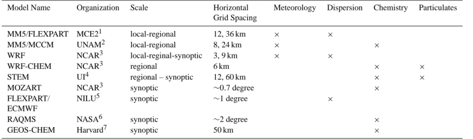
The 700 hPa wind and geopotential height fields at 12:00 UTC every other day during March 2006 are shown in Fig. 3 to illustrate the evolving synoptic conditions dur-ing MILAGRO. While the 700 hPa level is ∼3200 m above sea level, it is only ∼1000 m above the ground over Mexico City. During the first part of the field campaign between 1 and 8 March (Figs. 3a–d), high pressure at 700 hPa slowly
1 181 361 540 720 900 1 181 361 540 720 900
(a) 12 UTC March 1
3000 3060 3120
H
1 181 361 540 720 900 1 181 361 540 720 900 1 181 361 540 720 900 1 181 361 540 720 900 (b) 12 UTC March 3 3000 3000 3060 3120H
L
L
1 181 361 540 720 900 1 181 361 540 720 900 1 181 361 540 720 900 1 181 361 540 720 900 (c) 12 UTC March 5 3000 3000 3060 3120H
1 181 361 540 720 900 1 181 361 540 720 900 1 181 361 540 720 900 1 181 361 540 720 900 (d) 12 UTC March 7 3000 3060 3120H
1 181 361 540 720 900 1 181 361 540 720 900 1 181 361 540 720 900 1 181 361 540 720 900(e) 12 UTC March 9
3000 3060 3120
H
1 181 361 540 720 900 1 181 361 540 720 900 1 181 361 540 720 900 1 181 361 540 720 900 (f) 12 UTC March 11 3000 3060 3120L
H
1 181 361 540 720 900 1 181 361 540 720 900 1 181 361 540 720 900 1 181 361 540 720 900 (g) 12 UTC March 13 3000 3060 3120L
H
1 181 361 540 720 900 1 181 361 540 720 900 1 181 361 540 720 900 1 181 361 540 720 900 (h) 12 UTC March 15 3000 3060 3120H
1 181 361 540 720 900 1 181 361 540 720 900 1 181 361 540 720 900 1 181 361 540 720 900(i) 12 UTC March 17
3000 3000 3060 3120 3120
H
L
1 181 361 540 720 900 1 181 361 540 720 900 1 181 361 540 720 900 1 181 361 540 720 900 (j) 12 UTC March 19 3000 3000 3060 3120L
H
1 181 361 540 720 900 1 181 361 540 720 900 1 181 361 540 720 900 1 181 361 540 720 900 (k) 12 UTC March 21 3000 3000 3060 3120L
H
1 181 361 540 720 900 1 181 361 540 720 900 1 181 361 540 720 900 1 181 361 540 720 900 (l) 12 UTC March 23 3000 3000 3060 3060 3120 3120 3120H
1 181 361 540 720 900 1 181 361 540 720 900 1 181 361 540 720 900 1 181 361 540 720 900 (m) 12 UTC March 25 3000 3000 3060 3120L
L
H
1 181 361 540 720 900 1 181 361 540 720 900 1 181 361 540 720 900 1 181 361 540 720 900 (n) 12 UTC March 27 3000 3060 3120H
L
1 181 361 540 720 900 1 181 361 540 720 900 1 181 361 540 720 900 1 181 361 540 720 900(o) 12 UTC March 29
3000 3060 3120
H
L
1 181 361 540 720 900 1 181 361 540 720 900 < 3 3 - 6 6 - 9 9 - 12 12 - 15 15 - 18.0 > 18.0 m s-1Fig. 3. Winds (arrows) and geopotential heights (contours) at 700 hPa at 12:00 UTC for every-other day during the field campaign period
1 3 5 7 9 11 13 15 17 19 21 23 25 27 29 31 date (UTC) 0 5 10 15 20 700 hPA speed (m s -1) 1 3 5 7 9 11 13 15 17 19 21 23 25 27 29 31 date (UTC) 0 90 180 270 360
700 hPA direction (deg)
1 3 5 7 9 11 13 15 17 19 21 23 25 27 29 31 0 90 180 270 360
700 hPA direction (deg)
1 3 5 7 9 11 13 15 17 19 21 23 25 27 29 31 0 5 10 15 20 500 hPA speed (m s -1) 1 3 5 7 9 11 13 15 17 19 21 23 25 27 29 31 0 90 180 270 360
500 hPA direction (deg)
1 3 5 7 9 11 13 15 17 19 21 23 25 27 29 31 date (UTC) 0 90 180 270 360
500 hPA direction (deg)
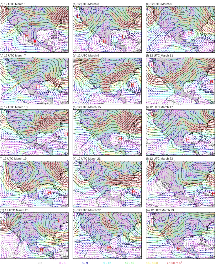
Fig. 4. Wind speed and direction at the 700 (bottom) and 500 hPa (top) levels over Mexico City from the rawinsondes (dots) and GFS
analyses closest to Mexico City (line). Gray shading denotes values from the GFS analyses within 0.5 degrees of Mexico City. Gray shading along the x-axis denotes periods with wind directions between 195 and 255 degrees that are favorable for transport from Mexico City to the T1 and T2 surface sampling sites.
moved from northwestern Mexico towards the east so that the winds over Mexico City were from the north and east. These synoptic conditions would transport Mexico City pol-lutants towards the Pacific Ocean. However, the clockwise circulation would eventually transport these pollutants back over Mexico. An upper-level trough propagating through the south-central U.S. on 9 March (Fig. 3e) produced westerly winds over Mexico. The winds became southwesterly be-tween 10 and 12 March (Fig. 3f) as a trough developed over the western U.S. After this trough moved over the north-central U.S. on 13 March (Fig. 3g), the winds over
cen-tral Mexico became light and variable. Between 14 and
18 March (Figs. 3h–i) a series of troughs and ridges prop-agated from west to east across the U.S. that affected the position of the high pressure system over the Gulf of ico and lead to variable wind directions over central
Mex-ico. A stronger trough propagated into the south-central
U.S., producing stronger southwesterly winds between 19 and 20 March (Fig. 3j). After 21 March (Figs. 3k–o), high pressure gradually developed over southern Mexico that pro-duced westerly winds at this level over central Mexico for the rest of the month.
The time series of wind speed and direction at the 700 and 500 hPa levels for the GFS grid point closest to Mexico City is shown in Fig. 4. The wind directions at 500 hPa were gen-erally northerly or easterly prior to 8 March. After the pas-sage of the upper-level trough on 9 March, the wind direc-tion became southwesterly and then southerly by 12 March.
Wind directions after 13 March gradually became westerly
by the end of the month. Wind speeds exceeding 15 m s−1
at 500 hPa were associated with the troughs during the 9–11 March and 19–20 March periods. Wind speeds at 700 hPa
were almost always less than 10 m s−1and usually less than
5 m s−1. Since the winds at 700 hPa are usually within the
boundary layer during the day, the directions exhibited more diurnal variation and horizontal variability than at 500 hPa.
The shading on the x-axis in Fig. 4 denotes periods of southwesterly wind directions between 195 and 255 degrees that were favorable for transport from Mexico City to the T1 and T2 sites. Transport was favorable ∼43% of the time at 700 hPa level and ∼36% of the time at the 500 hPa level during the month assuming the wind remains constant dur-ing the 6-h periods when GFS output and rawinsonde data was available. At other times, the T1 and T2 chemistry in-strumentation would likely sample either clean air, pollutants from sources other than Mexico City, or aged Mexico City pollutants recirculated around the region.
Also shown in Fig. 4 are the measurements from the Mex-ico City rawinsondes. While the GFS model wind directions at 500 hPa were very similar to those from the rawinsondes,
the wind speeds differed by as much as 5 m s−1. Relatively
large differences in both speed and direction were evident at the 700-hPa level. Some differences are to be expected since the 0.5-degree grid spacing does not resolve the ter-rain variations of the Mexican plateau that affect the devel-opment of near-surface circulations. In addition, the seven
1 3 5 7 9 11 13 15 17 19 21 23 25 27 29 31 0 5 10 15 20 25 975 hPA speed (m s -1)
Norte 1 Norte 2 Norte 3
1 3 5 7 9 11 13 15 17 19 21 23 25 27 29 31 date (UTC) 0 90 180 270 360
975 hPA direction (deg)
1 3 5 7 9 11 13 15 17 19 21 23 25 27 29 31 0 90 180 270 360
975 hPA direction (deg)
Fig. 5. Wind speed (top) and direction (bottom) at Veracruz during March 2006 from the rawinsondes (white dots), radar wind profiler (black
dots), and GFS analysis grid point closet to Veracruz (line). Values from the GFS analyses and radiosondes are from the 975 hPa level and measurements from the radar wind profiler are at 400 m a.g.l. Gray shading denotes GFS values within one degree of Veracruz.
vertical levels in the GFS analyses below 850 hPa may not fully resolve the vertical variations observed by the rawin-sondes. Quality control algorithms may also discard
“non-representative” near-surface measurements. It is possible
that some of the rawinsondes at 06:00 and 18:00 UTC were not assimilated into the large-scale analyses; however, there was no relationship between the magnitude of the differ-ence and time of day. A similar analysis performed for Ve-racruz where the terrain is relatively flat also produced rel-atively large differences between the GFS and rawinsondes both near the surface and aloft (not shown). This suggests a portion of the forecast errors produced by the MILAGRO regional models could be attributed to errors in the synoptic conditions from the GFS analyses.
5 Cold surge events
Strong northerly near-surface flows associated with the pas-sage of cold fronts over the Gulf of Mexico occurred three times after 14 March. Although cold fronts gradually dissi-pate as they propagate into the subtropics, the interaction of the southward moving high-pressure systems with the terrain of the Sierra Madre Oriental often accelerates the northerly flow along the coast. The propagation of strong northerly near-surface flow into the subtropics has been called a “ cold surge” (Schultz et al., 1997; Steenburgh et al., 1998), but is commonly known as a “Norte” event in Mexico (Mosino Aleman and Garcia, 1974). Here, we refer to the three cold front passages as Norte 1, Norte 2, and Norte 3. While northerly winds occurred over Mexico City after the passage of the fronts, the wind speeds were much lower than those
observed along the coast at lower elevations. In addition to affecting the local transport of pollutants over central Mex-ico, the Norte events increased humidity, cloudiness, and pre-cipitation that influence the transformation and removal of trace gases and aerosols.
As far as we know, the radar wind profiler at Veracruz provided the first detailed (temporal and vertical resolution) measurements of the Norte events in Mexico. Figure 5 shows the wind speed and direction from the Veracruz radar wind profiler during the field campaign at 400 m a.g.l., along with the wind speeds and directions from the rawinsonde and GFS analyses at the 975-hPa level that varied between 240 and 420 m a.g.l. The first Norte event occurred between 14 and 15 March with northerly wind speeds as high as
15 m s−1. While the second Norte lasted only several hours
on 22 March, wind speeds were as high at 20 m s−1. The
third Norte was the most significant with wind speeds up to
25 m s−1. It began on 23 March and strong northerly winds
persisted for two days after the frontal passage.
The measurements from the radar wind profiler and raw-insondes were very similar. While the temporal variations in the GFS model winds were qualitatively similar to the measurements, the wind speeds were lower than observed and the wind directions had more diurnal variation than ob-served. The GFS wind speeds and directions for surrounding grid points over the ocean were closer to the measurements, suggesting that the differences resulted primarily from issues associated with resolving the coast.
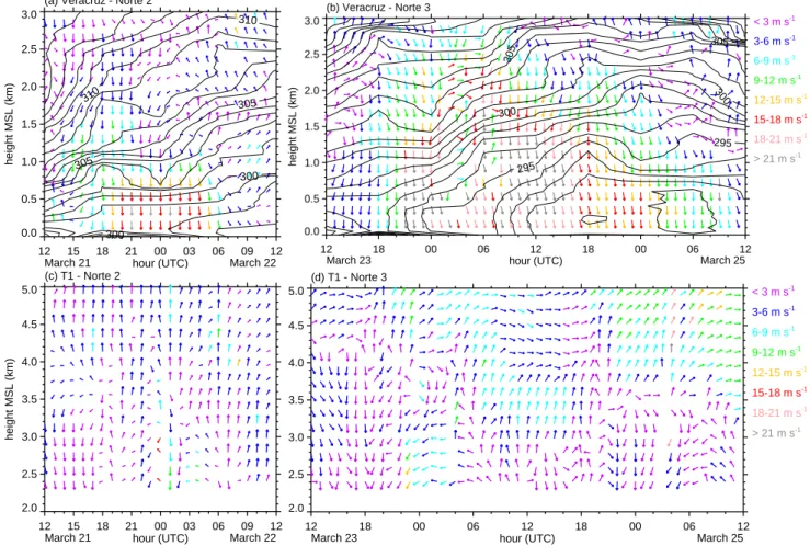
The vertical wind profiles in speed and direction from the Veracruz radar wind profiler during the second and third Norte events are shown in Fig. 6. The potential tempera-ture contours in this figure were obtained by temporal linear
12 15 18 21 00 03 06 09 12 hour (UTC) 0.0 0.5 1.0 1.5 2.0 2.5 3.0 height MSL (km) March 21 March 22
(a) Veracruz - Norte 2
300 300 305 305 310 310 12 18 00 06 12 18 00 06 12 hour (UTC) 0.0 0.5 1.0 1.5 2.0 2.5 3.0 height MSL (km) March 23 March 25 (b) Veracruz - Norte 3 295 295 300 300 305 305 < 3 m s-1 3-6 m s-1 6-9 m s-1 9-12 m s-1 12-15 m s-1 15-18 m s-1 18-21 m s-1 > 21 m s-1 12 15 18 21 00 03 06 09 12 hour (UTC) 2.0 2.5 3.0 3.5 4.0 4.5 5.0 height MSL (km) March 21 March 22 (c) T1 - Norte 2 12 18 00 06 12 18 00 06 12 hour (UTC) 2.0 2.5 3.0 3.5 4.0 4.5 5.0 March 23 March 25 (d) T1 - Norte 3 < 3 m s-1 3-6 m s-1 6-9 m s-1 9-12 m s-1 12-15 m s-1 15-18 m s-1 18-21 m s-1 > 21 m s-1
Fig. 6. Wind profiles from the Veracruz (a and b) and T1 (c and d) radar wind profilers during the second and third Norte. Black contours
denote potential temperature contours obtained by interpolating in time the Veracruz soundings available at 6-h intervals.
1 181 361 540 720 900 1 181 361 540 720 900
(a) 12 UTC March 23
1500 1500 1500 1500 1560 1560 1560
H
H
L
1 181 361 540 720 900 1 181 361 540 720 900 1 181 361 540 720 900 1 181 361 540 720 900 (b) 12 UTC March 24 1500 1500 1500 1500 1560 1560H
L
L
L
1 181 361 540 720 900 1 181 361 540 720 900 < 2.5 2.5 - 7.5 7.5 - 12.5 12.5 - 17.5 > 17.5 m s-1Fig. 7. 850 hPa geopotential heights (contours) and winds (arrows) during the third Norte at (a) 12:00 UTC 23 March and (b) 12:00 UTC 24
1 3 5 7 9 11 13 15 17 19 21 23 25 27 29 31 10 15 20 25 30 35 temperature (C) 1 3 5 7 9 11 13 15 17 19 21 23 25 27 29 31 10 15 20 25 30 35 temperature (C)
Norte 1 Norte 2 Norte 3
1 3 5 7 9 11 13 15 17 19 21 23 25 27 29 31 0 25 50 75 100 relative humidity (%) 1 3 5 7 9 11 13 15 17 19 21 23 25 27 29 31 0 25 50 75 100 relative humidity (%) 1 3 5 7 9 11 13 15 17 19 21 23 25 27 29 31 date 0 5 10 15 20 specific humidity (g kg -1)
Mexico City (dark blue), Pachuca (light blue), Veracruz (red)
1 3 5 7 9 11 13 15 17 19 21 23 25 27 29 31 date 0 5 10 15 20 specific humidity (g kg -1)
Fig. 8. Temperature (top), relative humidity (middle), and specific humidity (bottom) at Veracruz (gray), Pachuca (thin black) and Mexico
City (thick black) during the field campaign. Dark shading denotes periods influenced by Norte events at Veracruz.
interpolation of the rawinsonde temperature profiles col-lected every six hours. During the second Norte (Fig. 6a),
wind speeds greater than 12 m s−1 occurred within 0.6 km
of ground between 19:00 UTC 21 March and 05:00 UTC 22 March. Mechanical mixing associated with the strongest winds contributed to the near-neutral layer within 0.4 km of the ground. The third Norte event (Fig. 6b) had stronger wind speeds over a much greater depth. Wind speeds
exceed-ing 12 m s−1extended up to 2.5 km m.s.l. a few hours after
the passage of the front. Despite the high wind speeds, me-chanical mixing produced a neutral layer only in the lowest few hundred meters. Wind speeds gradually diminish after 12:00 UTC 25 March, but remain northerly until 19:00 UTC 26 March. Northerly flows at T1 for the second (Fig. 6c) and third (Fig. 6d) Norte were much weaker and of shorter duration.
The winds and geopotenial heights at the 850 hPa level at two times are shown in Fig. 7 to illustrate the synop-tic conditions just prior to the arrival of the front at Ver-acruz at 12:00 UTC 23 March and during the third Norte at 12:00 UTC 24 March. At 12:00 UTC 23 March (Fig. 7a),
northerly winds between 10 and 17.5 m s−1 occurred over
the Great Plains from northern Canada into northern Mex-ico as a result of a strong pressure gradient across the central
U.S. Surface temperatures dropped below 0◦C as far south as
Texas. After the front moved past Veracruz (Fig. 7b) strong northerly and northwesterly winds were present over the en-tire Gulf of Mexico. The winds accelerated to greater than
20 m s−1through the terrain gap in the southern isthmus of
Mexico and over the Gulf of Tehuantepec. The synoptic
con-ditions, gap winds, and cloud distribution for this Norte were very similar to the cold surge of 12–14 March 1993 described by Steenburgh et al. (1998).
The effects of the three Norte events on the 2-m temper-ature, relative humidity, and specific humidity at Veracruz, Pachuca, and Mexico City are shown in Fig. 8. Tempera-tures over the coast were higher and have less diurnal range than temperatures over the plateau, as expected. Daily max-imum temperatures during each Norte drop a few degrees from the preceding days. During the first thirteen days of the field campaign the atmospheric moisture was very low over the plateau with relative humidities usually less than 50%
and mixing ratios less than 7 g kg−1. Afternoon relative
hu-midity and specific huhu-midity often dropped to less 10% and
3 g kg−1, respectively. During the first Norte, relative
humid-ity rose as the temperatures decreased and specific humidhumid-ity
increased to 8–10 g kg−1. Since there are no significant local
sources of moisture over the plateau, the increase of mois-ture must have been associated with transport from the Gulf of Mexico. While the humidity dropped somewhat after the first Norte, the relative and specific humidities were higher on average than during the dry period earlier in the month. Humidities over the plateau increased again during the sec-ond and third Norte events. Specific humidity was usually
between 7 to 10 g kg−1after the third Norte until the end of
the month.
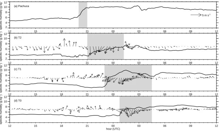
The transport of moisture from the Gulf of Mexico to-wards Mexico City for the second Norte is depicted in Fig. 9. A sharp increase in specific humidity was observed at Pachuca (Fig. 9a) between 20:00 and 21:00 UTC on 21
12 15 18 21 00 03 06 09 12 0.0 0.2 0.4 0.6 0.8 1.0 5 m s-1 12 15 18 21 00 03 06 09 12 2 4 6 8 10 12 specific humidity (g kg -1) (a) Pachuca 12 15 18 21 00 03 06 09 12 0.0 0.2 0.4 0.6 0.8 1.0 12 15 18 21 00 03 06 09 12 2 4 6 8 10 12 specific humidity (g kg -1) (b) T2 12 15 18 21 00 03 06 09 12 0.0 0.2 0.4 0.6 0.8 1.0 12 15 18 21 00 03 06 09 12 2 4 6 8 10 12 specific humidity (g kg -1) (c) T1 12 15 18 21 00 03 06 09 12 0.0 0.2 0.4 0.6 0.8 1.0 12 15 18 21 00 03 06 09 12 hour (UTC) 2 4 6 8 10 12 specific humidity (g kg -1) (d) T0
Fig. 9. Specific humidity and winds observed at (a) Pachuca, (b), T2, (c) T1, and (d) T0 between 12:00 UTC March 21 and 12:00 UTC 22
March. Shading denotes rise in humidity and shift to northerly winds associated with the start of the second Norte. Wind speeds at Pachuca were missing at this time.
March. Unfortunately, the wind measurements at Pachuca were missing for most of March. An increase in specific hu-midity was observed at T2 one hour later at 21:00 UTC and northerly winds were associated with the gradual increase in specific humidity over the next 3.5 h. The Norte arrived at T1 and T0 around 23:00 UTC 21 March and 00:30 UTC 22 March, respectively. The operational meteorological sites in Mexico City (Fig. 2b) indicated that the northerly flow propagated to the southern end of the basin by 03:00 UTC (not shown). After the passage of the Norte, specific
humid-ity at T0 was 1–2 g kg−1lower than at Pachuca, suggesting
that mixing processes diluted the air mass as it was trans-ported over the plateau. These measurements indicate that the northerly winds propagated over central plateau from Pachuca to Mexico City in about 4.5 h at an average speed
of about 4.9 m s−1. The propagation of moisture over the
plateau for the first and third Nortes was similar to Fig. 9 (not shown).
The strong winds associated with the cold surges con-tributed to periods of wind-blown dust over the central plateau in addition to convective outflow and interactions of local and regional thermally-driven circulations.
Measure-ments of PM10 exceeded 300 µg m−3at a number of
oper-ational stations in Mexico City on 8, 9, 10, 13, 14, 16, 17,
18, 19, 20, 21, and 23 March. The highest PM10values
usu-ally occurred when near-surface wind speeds increased sig-nificantly over the eastern side of the valley where the dry and sparsely vegetated soil is susceptible to wind erosion. Because of the proximity of urban areas and dust emission sources, the evolution of particulates downwind of Mexico City was likely influenced by the interaction of mineral dust and anthropogenic trace gases.
6 Clouds and precipitation
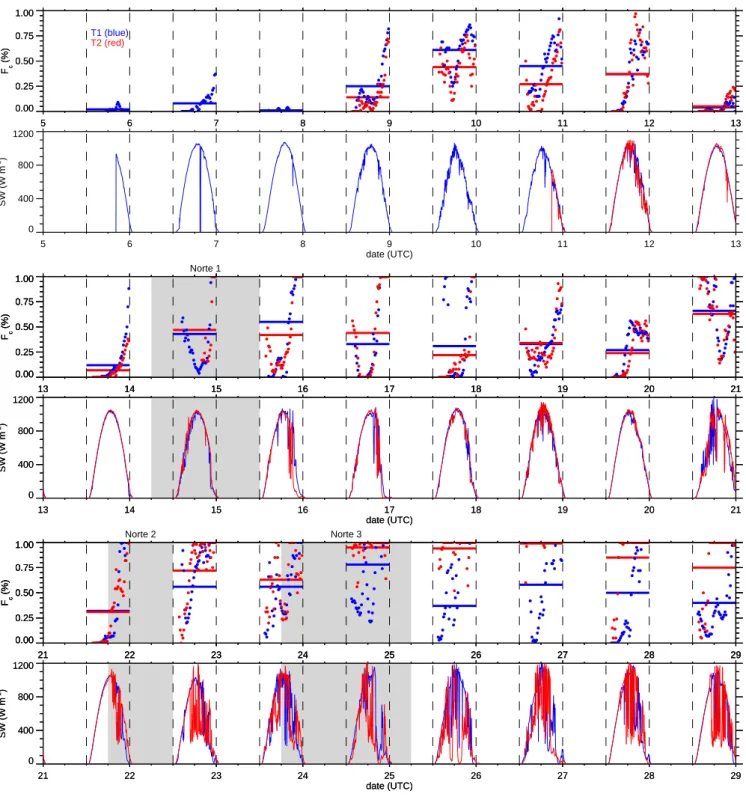
Not surprisingly, the passage of cold fronts and the increase in moisture led to increased cloudiness in the region. This is an important factor during MILAGRO because the scatter-ing and absorption of radiation by clouds reduces the tochemical production below cloud base and increases pho-tochemical production above cloud tops, vertical transport within clouds alters the distribution of pollutants, and precip-itation removes trace gases and particulates from the atmo-sphere. Table 2 qualitatively summarizes the daytime cloud conditions during the field campaign based on inspection of visible satellite images while Fig. 10 quantifies the
cloudi-ness at T1 and T2 by using fractional cloudicloudi-ness, Fc, derived
5 6 7 8 9 10 11 12 13 0.00 0.25 0.50 0.75 1.00 Fc (%) T1 (blue) T2 (red) 5 6 7 8 9 10 11 12 13 0.00 0.25 0.50 0.75 1.00 Fc (%) 13 14 15 16 17 18 19 20 21 0.00 0.25 0.50 0.75 1.00 Fc (%) Norte 1 13 14 15 16 17 18 19 20 21 0.00 0.25 0.50 0.75 1.00 Fc (%) 13 14 15 16 17 18 19 20 21 0.00 0.25 0.50 0.75 1.00 Fc (%) 21 22 23 24 25 26 27 28 29 0.00 0.25 0.50 0.75 1.00 Fc (%) Norte 2 Norte 3 21 22 23 24 25 26 27 28 29 0.00 0.25 0.50 0.75 1.00 Fc (%) 21 22 23 24 25 26 27 28 29 0.00 0.25 0.50 0.75 1.00 Fc (%) 5 6 7 8 9 10 11 12 13 date (UTC) 0 400 800 1200 SW (W m -2) 13 14 15 16 17 18 19 20 21 date (UTC) 0 400 800 1200 SW (W m -2) 13 14 15 16 17 18 19 20 21 date (UTC) 0 400 800 1200 SW (W m -2) 21 22 23 24 25 26 27 28 29 date (UTC) 0 400 800 1200 SW (W m -2) 21 22 23 24 25 26 27 28 29 date (UTC) 0 400 800 1200 SW (W m -2)
Fig. 10. Fractional cloudiness, Fc, and total downward shortwave radiation, SW, during the field campaign period at the T1 (blue) and T2
(red) site. Dots denote 15-min averages and thick horizontal lines denote afternoon averages of the fractional cloudiness. Shading denotes Norte periods and dashed lines denote sunrise and sunset.
measurements (Long et al., 2006) and total downward short-wave radiation, SW, from Eppley broadband radiometers. The variations in cloudiness and shortwave radiation at other nearby sites in Mexico City and Pachuca were similar to those shown in Fig. 10.
The high daily average shortwave radiation at T1 and T2 and other operational measurements indicates mostly sunny skies occurred over the central plateau between 1 and 13 March. Somewhat lower daily averages at stations located just east of the Sierra Madre Oriental (not shown) between 3
Table 2. Cloudiness during MILAGRO.
March T0-T1-T2 morning T0-T1-T2 afternoon Mountains in the vicinity of Mex-ico City
Deep convection Sierra Madre Oriental foothills Cirrus
1 CLR CLR PC ISO PC No 2 CLR CLR CLR none SCA No 3 CLR CLR CLR none PC No 4 CLR CLR CLR none PC No 5 CLR CLR CLR none MC No 6 CLR CLR CLR none PC No 7 CLR CLR CLR none SCA No 8 CLR CLR PC none CLR Yes 9 CLR CLR CLR none CLR Yes 10 CLR CLR CLR none CLR Yes 11 CLR CLR CLR none CLR Yes 12 CLR CLR PC none CLR Yes 13 CLR CLR PC ISO CLR No 14 CLR PC PC ISO MC No 15 CLR MC PC SCA PC No 16 CLR MC PC SCA PC No 17 CLR PC PC ISO PC Yes 18 CLR CLR PC none PC Yes 19 CLR CLR PC none SCA No 20 CLR CLR CLR none CLR Yes 21 CLR PC PC none PC Yes 22 CLR PC PC none PC No 23 CLR PC PC ISO MC No 24 CLR PC PC ISO MC No 25 PC PC PC none PC No 26 CLR PC PC ISO PC No 27 CLR PC PC ISO PC No 28 CLR PC PC ISO PC No 29 CLR PC PC ISO PC No 30 CLR PC PC ISO PC No 31 CLR PC PC ISO SCA No CLR = clear SCA = scattered PC = partly cloudy MC = mostly cloudy ISO = isolated
and 5 March were associated with marine stratus that formed along the eastern slopes of the plateau as a result of the north-easterly winds aloft (Figs. 3 and 4). Afternoon averaged
Fc was as large as 60% over the plateau between 9 and 13
March as a result of cirrus clouds transported into the region by upper-level southwesterly flow, but the cirrus clouds lead to only small reductions in downward solar radiation. In-creases in low-level clouds occurred during the first Norte on 14 March at all sites. After the Norte, mostly clear skies were usually observed over central Mexico during the morning, but the increased humidity provided favorable conditions for afternoon partly cloudy conditions to develop over the moun-tain ranges and the plateau on several days between 15 and
21 March. Fc at T1 and T2 was quite similar during this
period. While clear skies were usually observed during the morning in the vicinity of Mexico City for the remainder of the month, the second and third Norte events led to periods of mostly cloudy conditions along the coast and increases in afternoon cloudiness over the plateau. After the third Norte, the increased humidity and synoptic conditions were favor-able for continued afternoon partly cloudy conditions in the
region and Fc at T2 became significantly larger than at T1.
Two factors likely contributed to the higher cloudiness at T2: the location of the site closer to regions of orographic uplift and decreased atmospheric static stability, as will be shown later.
Mexico City Veracruz
Pacific Ocean Pacific Ocean
Gulf of Mexico Gulf of Mexico
dust
gust front
(a) Terra Satellite: ~1630 UTC March 21 (b) Aqua Satellite: 1930 UTC March 24
plateau edge
convection preferrentially forming over mountains
Fig. 11. MODIS satellite image during the (a) second and (b) third Norte.
MODIS visible satellite images at ∼16:30 UTC on 21 March and ∼20:10 UTC 24 March are shown in Fig. 11 to illustrate the spatial distribution of cloudiness over central Mexico during the second and third Norte. At 16:30 UTC on 21 March, the strong near-surface northerly winds began to increase at Veracruz and produced blowing dust along the coast (Fig. 11a). Partly to mostly cloudy conditions occurred behind the front over the Gulf of Mexico and the coastal plain, while mostly sunny conditions were observed over the rest of Mexico. More widespread cloudiness was asso-ciated with the stronger third Norte. Mostly cloudy condi-tions were produced over the Gulf of Mexico, with the west-ern boundary along the Sierra Madre Oriental at approxi-mately 2 km m.s.l. (Fig. 11b). The increased moisture pro-duced partly cloudy conditions over the plateau, primarily over mountain ranges.
The increases in humidity and the morning clear-sky in-solation over the plateau after 14 March were favorable for thermally-driven slope flows so that shallow and deep con-vective clouds developed preferentially over the highest ter-rain during the afternoon. Satellite images indicated that deep convection occurred over the central plateau during the afternoons of 13–17 March, 23–24 March and 25–31 March. The stability of the atmosphere also decreased during these periods as shown in Fig. 12a by the K index derived from the rawinsondes at Mexico City. The K index is a simple index derived from vertical temperature and moisture gradients be-low 500 hPa (George, 1960). In general, higher values of K indicate an increased probability of air mass thunderstorms. Values greater than 28 have been used to indicate a 50% or greater probability, but various studies have found different
specific probabilities using the K index. This index also does not account for convergence resulting from the topographic variations and thermally-driven circulations over the plateau that would enhance convective instability in certain regions. The K index is low during the first part of the field cam-paign between 2 and 13 March when clear skies were usu-ally observed. Increases in the K index and precipitable wa-ter (Fig. 12b) were associated with each of the Norte events. The K index remained high after the third Norte, indicating that conditions over the plateau were favorable for convective activity.
The increased cloudiness was also accompanied by scat-tered precipitation, as shown by the precipitation within the Mexico basin and at Pachuca in Fig. 12c, and the accumu-lated precipitation prior to and after the second Norte, as shown in Fig. 13. Light rain was observed in Mexico City and at Pachuca after the second Norte (Fig. 12c). The pre-cipitation usually occurred during the late afternoon within a few hours after sunset. Although precipitation was not ob-served between 13 and 17 March, scattered convection in the region produced rainfall at other locations. Hail and light-ning were observed in the vicinity of T1 on 16 March.
As shown in Fig. 13, precipitation before 21 March was light with only five stations in central Mexico reporting rain-fall exceeding 3 mm (Fig. 13a). Most of this precipitation was associated with isolated deep convective activity after the first Norte on 14 March (Table 2). After 22 March, pre-cipitation was observed at most stations in central Mexico (Fig. 13b). The increased frequency of convective activity associated with the third Norte led to precipitation exceed-ing 18 mm at five stations. The increased cloudiness and
1 3 5 7 9 11 13 15 17 19 21 23 25 27 29 31 -10 0 10 20 30 40 K Index
(a) Norte 1 Norte 2 Norte 3
1 3 5 7 9 11 13 15 17 19 21 23 25 27 29 31 -10 0 10 20 30 40 K Index 1 3 5 7 9 11 13 15 17 19 21 23 25 27 29 31 0 5 10 15 20 precipitable water (mm) (b) 1 3 5 7 9 11 13 15 17 19 21 23 25 27 29 31 0 5 10 15 20 precipitable water (mm) 1 3 5 7 9 11 13 15 17 19 21 23 25 27 29 31 date (UTC) 0 2 4 6 8 precipitation (mm) (c) 1 3 5 7 9 11 13 15 17 19 21 23 25 27 29 31 date (UTC) 0 2 4 6 8 precipitation (mm)
Fig. 12. (a) K index and (b) precipitable water from the Mexico City soundings and (c) precipitation from stations in the vicinity of Mexico
City (black dots) and at Pachuca (white dots). Dots in (a) and (b) are for the 18:00 and 00:00 UTC soundings to highlight afternoon periods. Light gray denotes Norte events and dark gray denotes afternoons when convective activity occurred over the central plateau.
1 181 361 540 720 900 1 181 361 540 720 900
(a) accumulated precipitation March 1 - 20
Mexico City 1 181 361 540 720 900 1 181 361 540 720 900
(b) accumulated precipitation March 21 - 31
Mexico City 0 - 3 3 - 6 6 - 9 9 - 12 12 - 15 15 - 18 > 18 mm
Fig. 13. Accumulated precipitation over Mexico between (a) 1 and 21 March and (b) 22 and 31 March corresponding to periods before and
after Norte event 1.
precipitation during the later part of the month also increases the possibility of the pollutants being diluted by convective transport and wet scavenging downwind of Mexico City.
7 Biomass burning
The month of March was also chosen as the MILAGRO ex-perimental period because the number of fires is normally
1 181 361 540 720 900 1 181 361 540 720 900
(a) fires between March 1 and 20
Mexico City 1 181 361 540 720 900 1 181 361 540 720 900
(b) fires between March 21 and 31
Mexico City
white: < 100 Mg CO day-1 gray: 100 - 1000 Mg CO day-1 black: > 1000 Mg CO day-1
Fig. 14. Fires before and after Norte event 2 as derived from MODIS satellite images as described by Wiedinmyer et al. (2006).
relatively low during this month. Most planned and
un-planned biomass burning in Mexico occurs between March and June, with the peak number of fires occurring during May (Wiedinmyer et al., 2006). In this way, scientists could focus on the evolution of the Mexico City pollutants with-out the complications of trace gases and aerosols from fire sources mixing with and altering the evolution of the Mexico City plume. Smoke would also alter atmospheric chemistry and contribute to the aerosol optical depth in the vicinity of Mexico City. However, a number of fires that likely con-tributed to poorer air quality and visibility occurred in central Mexico during March 2006, as reported by scientists on the research aircraft and by satellite images.
Daily estimates of trace gas and particulate emissions from fires were made using the MODIS thermal anomalies prod-uct and land cover information as described by Wiedinmyer et al. (2006). Terra and Aqua satellites pass over or near Mex-ico twice a day so that this methodology can miss short-lived fires. Many fires observed, for example by the USFS aircraft, were small shrub and agricultural clearing fires that were not detected by satellite. Carbon monoxide emissions from fires before and after 21 March are shown in Fig. 14. Prior to the second Norte during dry conditions with clear skies, numer-ous fires were observed throughout Mexico (Fig. 14a). Many of these fires occurred in the vicinity of Mexico City with emissions of carbon monoxide from several estimated to
ex-ceed 1000 Mg day−1. MODIS satellite images showed that
many of these smoke plumes were close to Mexico City. Not surprisingly, the increased cloudiness and precipitation over
central Mexico (Figs. 10 and 13) led to fewer fires with sig-nificantly lower emissions after the second Norte (Fig. 14b). The number of fires in Fig. 14b may be underestimated since the clouds would also obscure fires from the satellite measurements. Nevertheless, the results show that there was a greater probability of interactions between the Mexico City plume and biomass burning smoke plumes during the first three weeks of MILAGRO. The relative contribution of an-thropogenic and biomass burning sources to the aerosol opti-cal properties will be determined by future measurement and modeling studies of atmospheric chemistry.
8 Regional-scale boundary layer structure and winds
Whiteman et al. (2000) quantified the average horizon-tal temperature and humidity gradients between the central plateau and the surrounding free atmosphere by employing the radiosonde measurements obtained from Mexico City and the coastal regions surrounding the plateau at 12:00 and 00:00 UTC during March 1997. A similar analysis of the mean profiles during MILAGRO is shown in Fig. 15, except that the four-times per day soundings permit average pro-files at 06:00 and 18:00 UTC to be included in the diurnal variations. At 18:00 UTC, the growing convective boundary layer (CBL) over Mexico City produced near-surface tem-peratures that were warmer than the surrounding free atmo-sphere. By 00:00 UTC, the average mixed layer height was
∼5 km m.s.l. (∼2.6 km a.g.l.). Potential temperatures east
290 300 310 320 330 potential temperature (K) 0 1 2 3 4 5 6 7 8 height MSL (km) 18 UTC Mexico City Veracruz Acapulco 290 300 310 320 330 potential temperature (K) 0 1 2 3 4 5 6 7 8 00 UTC 290 300 310 320 330 potential temperature (K) 0 1 2 3 4 5 6 7 8 06 UTC 290 300 310 320 330 potential temperature (K) 0 1 2 3 4 5 6 7 8 12 UTC 0 4 8 12 16 specific humidity (g kg-1 ) 0 1 2 3 4 5 6 7 8 height MSL (km) 18 UTC 0 4 8 12 16 specific humidity (g kg-1 ) 0 1 2 3 4 5 6 7 8 00 UTC 0 4 8 12 16 specific humidity (g kg-1 ) 0 1 2 3 4 5 6 7 8 06 UTC 0 4 8 12 16 specific humidity (g kg-1 ) 0 1 2 3 4 5 6 7 8 12 UTC
Fig. 15. Average potential temperature and specific humidity profiles at 6-h intervals from the Mexico City, Veracruz, and Acapulco
rawin-sondes during the field campaign. The dashed line denotes the elevation of the Mexico City basin.
respectively, were almost identical. The CBL over the basin produces regional horizontal temperature gradients that drive the regional-scale circulations. Smaller-scale heating and ter-rain geometry associated with the mountain ranges leads to local-scale circulations. The specific humidity profiles in Fig. 15 show an increase in moisture above the plateau during the daytime. Since there are no significant moisture sources on the plateau itself and the growing CBL would entrain drier air into the mixed layer, the profiles suggest that advection from the surrounding coastal regions was responsible for this moistening.
After sunset, the CBL collapsed so that by morning (around 12:00 UTC) the potential temperatures at Mexico City were nearly identical to those at Veracruz and Acapulco at the same elevation. The soundings at 06:00 UTC, for a time period unavailable to Whiteman et al. (2000), provided evidence that while most cooling occurred on average be-tween 00:00 and 06:00 UTC, the basin was still somewhat warmer than the surrounding free atmosphere at the same el-evation at 06:00 UTC.
The potential temperature and specific humidity profiles were averaged between 1 and 20 March and 21–31 March to determine differences in the heating of the central plateau
before and after the second Norte, as shown in Fig. 16. Af-ter 21 March, potential temperatures decreased and specific humidities increased over both Mexico City and Veracruz as a result of the third and strongest Norte. During the drier and warmer period prior to the second Norte, the average boundary layer depth over Mexico City was about 500 m at 18:00 UTC. After the second Norte, the vertical poten-tial temperature gradient between 3 and 5 km m.s.l. deceased significantly. During the late afternoon at 00:00 UTC, the average boundary layer potential temperatures were 4–5 K cooler and the mixed layer depth was about 1 km lower af-ter the second Norte. A capping inversion between 5 and 5.5 km m.s.l. often formed during the night by 12:00 UTC after the second Norte. The specific humidity at Veracruz did not change significantly after the second Norte below about 2 km m.s.l.; however the average specific humidity increased
by as much as 3–4 g kg−1from the height of the plateau up
to 7 km m.s.l. at both Veracruz and Mexico City. The raw-insonde measurements suggest that the changes in humidity occurred in the entire region and that the synoptic conditions after the second Norte altered the growth of the CBL and the near-surface stability over the basin.
290 300 310 320 330 potential temperature (K) 0 1 2 3 4 5 6 7 8 height MSL (km) 18 UTC Mexico City Veracruz thin = March 1 - 20 thick = March 21 - 31 290 300 310 320 330 potential temperature (K) 0 1 2 3 4 5 6 7 8 00 UTC 290 300 310 320 330 potential temperature (K) 0 1 2 3 4 5 6 7 8 06 UTC 290 300 310 320 330 potential temperature (K) 0 1 2 3 4 5 6 7 8 12 UTC 0 4 8 12 16 specific humidity (g kg-1 ) 0 1 2 3 4 5 6 7 8 height MSL (km) 18 UTC 0 4 8 12 16 specific humidity (g kg-1 ) 0 1 2 3 4 5 6 7 8 00 UTC 0 4 8 12 16 specific humidity (g kg-1 ) 0 1 2 3 4 5 6 7 8 06 UTC 0 4 8 12 16 specific humidity (g kg-1 ) 0 1 2 3 4 5 6 7 8 12 UTC
Fig. 16. Same as Fig. 15, except average potential temperature and specific humidity profiles before and after the second Norte at Mexico
City and Veracruz. Thin and thick lines denote 1–20 March and 21–31 March periods, respectively.
A similar analysis was performed by averaging the raw-insonde profiles among three groups: those before the first Norte, those between the first and second Norte, and those after the second Norte. The resulting profiles showed a slight decrease in potential temperatures and increase in specific humidity after the first Norte (not shown), but that the largest changes occurred after the second and third Nortes.
High-pressure systems, weak synoptic forcing in the sub-tropics, and the horizontal temperature gradients over the central Mexican plateau (Figs. 15 and 14) are favorable for the development of local and regional thermally-driven flows (e.g. Bossert, 1997; Doran and Zhong, 2000; Whiteman et al., 2000) in the vicinity of Mexico City that affect the trans-port and mixing of pollutants. However, the local and re-gional winds will be suppressed when the synoptic forcing is sufficiently strong.
Wind profiler measurements at T0 and T1 are shown in Fig. 17 to indicate how often the diurnal thermally-driven winds over the central plateau (i.e. Fig. 1) are affected by the synoptic-scale forcing. There were two multi-day peri-ods at T0 and T1 in which neither the near-surface nor the upper-level wind directions at 400 and 1500 m a.g.l.,
respec-tively, exhibited diurnal variations with strong vertical wind shears and were both similar to the 500-hPa wind directions (Fig. 4). The strongest 500-hPa wind speeds during March occurred during these periods. The first period was between 9 and 11 March when the 500-hPa winds were southwest-erly, and the second period was between 18 and 20 March when the 500-hPa winds were southerly. While the wind di-rections at T0 and T1 during the second period were very similar, wind directions at T0 and T1 occasionally differed by as much as 80 degrees during the first period. This sug-gests that an interaction of the ambient wind direction and the mountain ranges surrounding Mexico City may affect the extent of vertical coupling of the basin and synoptic winds. The wind directions at 1500 m a.g.l. at T0 generally exhibit more temporal variability than at T1, indicating that the basin topography affects the vertical wind structure to a greater ex-tent over the city than over the more open terrain surrounding T1.
The radar wind profiler measurements in Fig. 17 show that there were many periods favorable for the transport of pollu-tants from Mexico City towards the northeast to the T1 and T2 sampling sites, as indicated by wind directions between
1 3 5 7 9 11 13 15 17 19 21 23 25 27 29 31 date 0 90 180 270 360 direction (deg)
(b) T0 radar wind profiler
1 3 5 7 9 11 13 15 17 19 21 23 25 27 29 31 date 0 90 180 270 360 direction (deg) 1 3 5 7 9 11 13 15 17 19 21 23 25 27 29 31 0 90 180 270 360 direction
(a) T1 radar wind profiler
1 3 5 7 9 11 13 15 17 19 21 23 25 27 29 31 0 90 180 270 360 direction
(a) T1 radar wind profiler
Fig. 17. Wind direction measured by radar wind profiles at the 400 m (blue dots) and 1500 m (red dots) a.g.l. range gates at the (a) T1 and (b) T0 sites. Black line denotes the 500 hPa-level wind speed and direction from the GFS grid point closed to Mexico City and gray shading
denotes nighttime periods. Gray shading along the x-axis denotes periods with directions between 195 and 255 degrees that are favorable for transport from Mexico City to the T1 and T2 sampling sites.
195 and 255 degrees. The periods in which the winds were within this range at T1 are also similar to the periods ob-tained from the Mexico City rawinsondes as shown in Fig. 4. However, the periods favorable for northeast transport at T0 were significantly shorter. The local winds near the surface, especially those within the basin, were obviously more com-plex than indicated by routine synoptic observations. Some of the differences between Figs. 4 and 17 result from the raw-insonde sampling interval every 6 h and the profiler sampling period of 30-min.
While increases in trace gases and aerosols measured at T1 and T2 will also indicate when transport from Mexico City occurred, dilution of the Mexico City plume and transport from other pollutant sources will complicate the interpreta-tion of chemistry data. Initial analyses (J. C. Doran, personal communication) indicated that it was often difficult to at-tribute small increases in black carbon and organic carbon to the Mexico City plume. High-resolution models that are con-strained by meteorological measurements and coupled with dispersion models will be needed to adequately describe the transport pathways and dilution by vertical mixing.
A more detailed analysis of boundary layer properties measured by the radar wind profilers, radiosondes, and lidars at the T0, T1, and T2 sites as well as an analysis of how local-scale circulations within the Valley of Mexico affect pollutant transport will be the subject of up-coming papers.
9 Transport
A series of tracer simulations were performed using the WRF-chem model (Grell et al., 2005; Fast et al., 2006) for March 1997, 2001, 2004, 2005, and 2006 to 1) determine whether the synoptic conditions observed during March 2006 were typical or anomalous and 2) illustrate the large-scale transport pathways. Three domains were employed, with the outer domain encompassing most of Mexico and the sur-rounding ocean with a grid spacing of 22.5 km, a second do-main encompassing central Mexico with a grid spacing of 7.5 km, and a third domain encompassing the Mexico City basin and areas to the northeast with a grid spacing of 2.5 km. The model was run in a tracer mode that simulated the emis-sion and transport of carbon monoxide (CO) with no chemi-cal reactions. The emission rates of CO, e CO, from Mexico City were based on a 1998 inventory. Since no estimates were available on regional scales outside of the basin, the to-tal CO emission rates for cities of 100 000 people or more were based on population such that
e COi =e COMC
populationi
populationMC (1)
where MC stands for Mexico City and i is the index for each city. Since Mexico City is by far the largest urban area, it was also the largest CO source.
The “footprint” of the CO plume during the entire month for each year is shown in Fig. 18. The footprint, FP, was
1 15 28 42 55 69 1 15 28 42 55 69 (a) March 1997 Gulf of Mexico Pacific Ocean 1 15 28 42 55 69 1 15 28 42 55 69 (b) March 2001 Gulf of Mexico Pacific Ocean 1 15 28 42 55 69 1 15 28 42 55 69 (c) March 2003 Gulf of Mexico Pacific Ocean 1 15 28 42 55 69 1 15 28 42 55 69 (d) March 2004 Gulf of Mexico Pacific Ocean 1 15 28 42 55 69 1 15 28 42 55 69 (e) March 2005 Gulf of Mexico Pacific Ocean 1 15 28 42 55 69 1 15 28 42 55 69 (f) March 2006 Gulf of Mexico Pacific Ocean 0.0 0.2 0.4 0.6 0.8 1.0 0.0 0.2 0.4 0.6 0.8 1.0 1 2 5 10 20 50 100 200 500 1000 e+03 ppm day-1
Fig. 18. The “footprint” of CO over Mexico averaged between 4.0 and 6.0 km m.s.l. obtained from WRF-chem tracer simulations for six
March periods. Black contours denote topography and white dot denotes Mexico City.
obtained using the following relationship:
F P (x, y) = 1 nt nt X l=1 nz X k=1 C(x, y, k, l)1z, for 4 ≤ z ≤ 6 km m.s.l. (2)
where x and y are the horizontal spatial locations, C is the mixing ratio of CO, 1z is the vertical grid spacing, nz is the number of vertical levels, and nt is the number of hours dur-ing the simulation period. The largest values of FP denote re-gions where the Mexico City plume passed through most fre-quently. The distribution of FP between 2.5 and 4 km m.s.l. was similar to the patterns shown in Fig. 18.
A common feature among five of the six simulations was the existence of two branches: one extending to the north-east over the Gulf of Mexico and the other extending to the southwest over the Pacific Ocean. The horizontal extent of these branches varied from year to year. The branch ex-tending over the Gulf of Mexico was associated with
high-pressure systems located east of Mexico City that produced transport towards the northeast (e.g. Fig. 3j). High-pressure systems located west of Mexico City that produced transport to the southwest were associated with the branch extending over the Pacific Ocean (e.g. Fig. 3a). The synoptic conditions during 1997 (Fig. 18a) and 2004 (Fig. 18d) frequently trans-ported Mexico City CO over the Pacific Ocean, but the syn-optic conditions during 2001 (Fig. 18b), 2003 (Fig. 18c), and 2006 (Fig. 18f) were not as favorable for transport towards the west. Transport towards the southwest did not occur at all at this altitude during 2005 (Fig. 18e) because a series of strong troughs propagated over Mexico the entire month; thus, March 2005 was most unlike the other periods. March of 2001, 2003, and 2004 had more CO transported towards the northeast over the Gulf of Mexico than during 2006. Al-though additional March periods need to be simulated to bet-ter establish a climatology of regional and long-range trans-port from Mexico City, the tracer analyses suggests that the synoptic conditions during March 2006 were not unusual.