Impact of gravity waves on the middle atmosphere of Mars: a non-orographic gravity wave parameterization based on Global Climate modeling and MCS observations

HAL Id: hal-02884115

https://hal.sorbonne-universite.fr/hal-02884115

Submitted on 29 Jun 2020

HAL is a multi-disciplinary open access

archive for the deposit and dissemination of

sci-entific research documents, whether they are

pub-lished or not. The documents may come from

teaching and research institutions in France or

abroad, or from public or private research centers.

L’archive ouverte pluridisciplinaire HAL, est

destinée au dépôt et à la diffusion de documents

scientifiques de niveau recherche, publiés ou non,

émanant des établissements d’enseignement et de

recherche français ou étrangers, des laboratoires

publics ou privés.

Mars: a non-orographic gravity wave parameterization

based on Global Climate modeling and MCS

observations

G. Gilli, F. Forget, A. Spiga, T. Navarro, E. Millour, L. Montabone, A.

Kleinböhl, D. Kass, D. Mccleese, J. Schofield

To cite this version:

G. Gilli, F. Forget, A. Spiga, T. Navarro, E. Millour, et al.. Impact of gravity waves on the middle

atmosphere of Mars: a non-orographic gravity wave parameterization based on Global Climate

mod-eling and MCS observations. Journal of Geophysical Research. Planets, Wiley-Blackwell, 2020, 125

(3), �10.1029/2018JE005873�. �hal-02884115�

Impact of gravity waves on the middle atmosphere of Mars: a

non-orographic gravity wave parameterization based on Global

Climate modeling and MCS observations

G. Gilli1,2_{, F. Forget}2_{, A. Spiga}2_{, T. Navarro}3_{, E. Millour}2_{, L. Montabone}2,4_{, A. Kleinböhl}5_{, D.} M. Kass5, D. J. McCleese6, J. T. Schofield5

1_{Instituto de Astrofísica e Ciências do Espaço (IA), Universidade de Lisboa, OAL, Tapada da Ajuda, PT1349-018 Lisboa,} Portugal

2_{Laboratoire de Météorologie Dynamique (LMD/IPSL), Centre National de la Recherche Scientifique, Sorbonne} Université, École Normale Supérieure, École Polytechnique, Paris, France

3_{Department of Earth, Planetary, and Space Sciences, University of California, Los Angeles, CA 90095-1567, USA} 4_{Space Science Institute, Boulder, Colorado, USA}

5_{Jet Propulsion Laboratory, California Institute of Technology, Pasadena, California, USA} 6_{California Institute of Technology, Pasadena, California, USA}

Key Points:

• _{A Stochastic non-orographic gravity wave (GW) scheme is implemented into the} LMD-MGCM

• _{Non-orographic GW generated above typical convective layers control diurnal tides}

• _{The implemented GW scheme improves the accuracy of the LMD-MGCM between 1}

and 0.01 Pa in comparison with MCS

Abstract

The impact of gravity waves (GW) on diurnal tides and the global circulation in the mid-dle/upper atmosphere of Mars is investigated using a General Circulation Model (GCM). We have implemented a stochastic parameterization of non-orographic GW into the Laboratoire de Météorologie Dynamique (LMD) Mars GCM (LMD-MGCM) following an innovative ap-proach. The source is assumed to be located above typical convective cells (∼ 250 Pa) and the effect of GW on the circulation and predicted thermal structure above 1 Pa (∼ 50 km) is analyzed. We focus on the comparison between model simulations and observations by the Mars Climate Sounder (MCS) on board Mars Reconnaissance Orbiter during Martian Year 29. MCS data provide the only systematic measurements of the Martian mesosphere up to 80 km to date. The primary effect of GW is to damp the thermal tides by reducing the diurnal oscillation of the meridional and zonal winds. The GW drag reaches magnitudes of the order of 1 m/s/sol above 10−2Pa in the northern hemisphere winter solstice and produces major changes in the zonal wind field (from tens to hundreds of m/s), while the impact on the tem-perature field is relatively moderate (10-20K). It suggests that GW induced alteration of the meridional flow is the main responsible for the simulated temperature variation. The results also show that with the GW scheme included, the maximum day-night temperature differ-ence due to the diurnal tide is around 10K, and the peak of the tide is shifted toward lower altitudes, in better agreement with MCS observations.

1 Introduction

Gravity waves (GW) are small-scale atmospheric waves frequently detected in terres-trial planet atmospheres. They are an intrinsic feature of all stably stratified planetary atmo-sphere and play an important role in the large-scale circulation and variability of the mid-dle/upper atmospheres of the Earth and Mars [Barnes, 1990; Joshi et al., 1995; Forget et al., 1999; Angelats i Coll et al., 2005; Fritts et al., 2006; Fritts and Alexander, 2003;

Alexan-der et al., 2010; Medvedev et al., 2011]. Depending on the source, GW can be excited in the

troposphere by a variety of mechanisms, which perturb the stratified atmospheric fluid and produce GW oscillations. The sources include flow over topography (orographic GW) or at-mospheric convection, front systems and jet-streams (non-orographic GW). The restoring force is the buoyancy that results from the adiabatic displacements of air parcels characteris-tic of these disturbances [Fritts and Alexander, 2003]. GW propagation into the atmosphere provides a significant source of momentum and energy to the mean flow when they break or encounter critical values. Thus, the gravity wave drag (i.e. gravity wave momentum deposi-tion to the mean flow) may cause wind acceleradeposi-tion or deceleradeposi-tion.

On the Earth, the observed reversal of the temperature gradient in the mesopause gion, resulting in a winter polar warming around the mesopause level (∼ 80-90 km), is

re-lated to the effects of GW drag on the global circulation [Lindzen, 1981; Holton, 1982; Hauchecorne

et al., 1987]. It is also well established that non-stationary (i.e. non-orographic) GW are

a substantial driver of the quasi-biennial oscillation (QBO) in the equatorial regions of the Earth’s atmosphere [Lindzen and Holton, 1968; Lott et al., 2012], complementing the forcing from the synoptic and planetary scale equatorial waves [Lott and Guez, 2013].

For Mars, several studies reported large density and temperature fluctuations (∼ 5 to 50 %) on small vertical scales height (<10 km vertically) from atmospheric entry profiles measured by Opportunity, Spirit, and Mars Pathfinder [Magalhães et al., 1999; Withers and

Smith, 2006; Holstein-Rathlou et al., 2016], as well as small horizontal scales (typically

20-300 km) in various Mars accelerometer data sets at aerobraking altitudes [Keating et al., 1998; Withers, 2006; Creasey et al., 2006a; Fritts et al., 2006] and from mass spectrome-ter measurements [Yiˇgit et al., 2015 and, Terada et al., 2017]. Radio occultation tempera-ture profiles by Mars Global Surveyor (MGS) obtained from the surface up to 35 km altitude also showed significant wave activity over the tropics, also partly attributed to zonally mod-ulated thermal tides [Hinson et al., 1999; Creasey et al., 2006b]. Furthermore, "rocket dust storms" during which rapid and efficient vertical transport takes place by injecting dust par-ticles at high altitudes in the Martian troposphere (30 to 50 km), may generate GW [Spiga

et al., 2013]. The role of mesoscale GW is supposed to be crucial for local CO2 condensa-tion, responsible for the formation of mesospheric CO2clouds observed by Mars Express between 60 and 80 km altitude [Spiga et al., 2012 and Montmessin et al., 2007].

MGS, Mars Odyssey (ODY) and Mars Reconnaissance Orbiter (MRO) aerobraking measurements were used to analyze density and temperature perturbations in the Martian thermosphere, where small-scale variability has been systematically observed whenever in situ data have been obtained (e.g. Keating et al. [2007]; Fritts et al. [2006]; Creasey et al. [2006a]; Zurek and Smrekar [2007]). MGS results (both radio profile and accelerometer data) leave open the question of the primary source mechanisms and source spectra, such as the distribution of phase speeds. Regarding the source, convection is often invoked to gen-erate non-orographic GW (e.g. non stationary waves with non-zero phase speed) which prop-agate upwards [Yiˇgit et al., 2015; Medvedev et al., 2011]. Fritts et al. [2006] and Creasey

et al.[2006a] found that GW amplitudes vary significantly with time and season, being

gen-erally larger in Northern autumn and winter (i.e. second half of Martian year), and at middle to high latitudes, apparently reflecting mean source and filtering conditions. Their ampli-tudes also appear to vary with longitude and time and may provide clues to interactions with larger-scale motions [Fritts et al., 2006]. According to Creasey et al. [2006b], westward-propagating waves may be encountering a critical level in spring and summer, but as the jet decreases towards autumn equinox, these waves may propagate to the thermosphere. More recently, NASA’s Neutral Gas Ion Mass Spectrometer (NGIMS) instrument aboard the Mars Atmosphere and Volatile EvolutioN (MAVEN) satellite retrieved large (20-40 %) GW-induced CO2density perturbations in the Mars upper atmosphere between 180 and 220 km [Yiˇgit et al., 2015]. Wave features were found with apparent wavelengths of ∼ 100 and 500 km in the Ar density around the exobase [Terada et al., 2017].

Many different parameterizations including those of Lindzen [1981]; Hines [1997] have been used to represent the impact of subgrid scale gravity wave processes in the ter-restrial atmosphere. For Mars, the inclusion of orographic GW effects improves the per-formance of models at lower and higher altitudes [Barnes, 1990; Collins et al., 1997;

For-get et al., 1999; Rafkin et al., 2001; Angelats i Coll et al., 2005]. Also, the thermal effect of

non-orographic gravity waves has been proposed to explain some of the puzzling model-observation discrepancy identified in the Martian atmosphere temperatures between 100 and 140 km [Medvedev and Yiˇgit, 2012], although a major part of the discrepancy can be attributed to issues in the calculation of the non-LTE radiative cooling by CO2[Forget et al., 2009; Medvedev et al., 2015]. Medvedev et al. [2015] implemented a nonlinear spectral grav-ity wave parameterization [Yiˇgit and Medvedev, 2010] in their GCM, extended up to 130 km, and their simulations showed that: 1. GW decelerate zonal winds at all seasons, 2. they produce jet reversals similar to those observed in the terrestrial mesosphere and lower ther-mosphere, 3. GW weaken the meridional wind and modify the zonal mean temperature by up to ± 15 K. However, modeling efforts for Mars suffer from lack of measurements to vali-date predicted wind fields and from no observational constraints on the GW forcing [Creasey

et al., 2006a] Other studies performed high-resolution simulations (∼ 60 km grid size) with a

general circulation model in order to resolve a significant portion of small-scale GWs and to capture the impact of GWs on the dynamics and energetics of Mars atmosphere without any parameterizations [Kuroda et al., 2015, 2016, 2019]. Those authors showed that the GW ac-tivity varies greatly with season and geographical location, with stronger wave generation in the northern hemisphere winter in the mesosphere and smaller activity in polar regions of the troposphere throughout all seasons. Given the lack of global observations of GW the clima-tology of the small-scale disturbances obtained in Kuroda et al. [2019] can serve as a proxy for gravity waves that are largely not resolved by GCMs with conventional grid resolution.

In this paper we describe the results of the implementation of a non-orographic GW parameterization into the Mars Global Climate Model (MGCM) developed at the Laboratoire de Météorologie Dynamique (LMD), which already included an orographic GW scheme [Forget et al., 1999]. Although the LMD-MGCM was already able to reproduce temperature observations with an error of less than 10 K at most locations and times, we found that it was

necessary to update the representation of several physical processes at work in the Martian atmosphere to further improve its accuracy. Among them: 1) the vertical distribution of the dust, characterized by detached layers (between 20 and 30 km) and by large day-night varia-tion [McCleese et al., 2010; Heavens et al., 2011a,b,c; Madeleine et al., 2011; Navarro et al., 2014], 2) the radiative impact of clouds, which remains challenging to be well represented in the GCM [Navarro et al., 2014], 3) the effect of GW (orographic and/or non-orographic), 4) the phasing of the thermal tide wave in the vertical compared to data from the Mars Cli-mate Sounder (MCS) on board MRO [Navarro et al., 2017]. MCS-MGCM biases probably resulted from the incorrect representation of the three previous processes mentioned above [Forget et al., 2017] and several improvements are currently being implemented.

Here we took advantage of the previous development work carried out by our team for the LMD Earth [Lott et al., 2012] and Venus GCM [Gilli et al., 2017] to also implement the same non-orographic GW scheme in the MGCM. According to Lott et al. [2012], the stochastic parameterization represents the unpredictable aspects of the sub-grid dynamics, considering that convection and fronts can generate waves throughout the full range of phase speeds, wave frequency, vertical and horizontal scales.In a context where the sources are not known precisely, we consider this is a reasonable choice. One of the main goals of this study is to understand the impact of non-orographic GW on the global circulation and the thermal structure of the Martian middle atmosphere (50-100 km altitude). What is the magnitude of GW-induced drag? Where do GW break/saturate and deposit the maximum momentum? Can GW explain the remaining discrepancy between the MCS observations and the GCM simulations? If so, what is their impact on the predicted winds?

Section 2 describes the non-orographic GW scheme and the main tunable parameters adopted in this work. The LMD-MGCM model and MCS dataset used here are described in Sections 3 and 4, respectively. The impact of our non-orographic GW scheme on the simu-lated wind and temperature is described in Section 5. The method implemented here to iden-tify the set of "best-fit" GW parameters is explained in Section 6, together with the compari-son with MCS results. A number of sensitivity tests is discussed in Section 7 and concluding remarks are given in the Section 8.

2 Non-orographic GW parameterization: formalism

The scheme implemented here is based on a stochastic approach, as fully described in Lott et al. [2012] and Lott and Guez [2013]. In such a scheme a finite number of waves (say M = 8), with characteristics chosen randomly, are launched upwards at each physical time-step (δt = 15 min) and at each horizontal grid point.The question of the location of the non-orographic GW sources is a difficult one and given the lack of information on such lo-cation, launching the gravity waves at each grid point is probably the simplest assumption. The number of waves is given as M = NK × NO × NP, with NK=2 values of GW horizontal wave-numbers, NO=2 absolute values of phase speed, and NP= 2 directions (westward and eastward) of phase speed. This approach allows the model to treat a large number of waves at a given time t by adding the effect of those M waves to that of the waves launched at pre-vious steps, to compute the tendencies. We need to parameterize GWs whose life cycle (i.e. from its generation to wave break) is contained in a characteristic time interval ∆t that has to significantly exceed the GCM time step δt. On the Earth, GW theory indicates that atmo-spheric disturbances induced by convection have life cycles with duration ∆t around 1 day (∆t = 24h) [Lott and Guez, 2013]. This typical time scale is likely to be relevant for Mars too: the choice for this timescale on Earth is made considering a mix of inertio-gravity waves (influenced by the planetary rotation, which is similar on both planets) and convectively-generated gravity waves, which have shorter frequency than the inertio-gravity waves, but which can propagate for several hours before dissipation or breaking occurs. The spectrum is discretized in 770 stochastic harmonics (≈ M x ∆t/δt) which contribute to the wave field each day and at a given horizontal grid point. At each time t the vertical velocity field w0of

an upward propagating GW can be represented by this sum: w0= ∞ X n=1 Cnw0n (1)

where Cnare normalization coefficients such thatP∞_n=1Cn2 = 1. It is assumed that each of the wn0 can be treated independently one from the others, and each Cn2can be viewed as the probability that wave field is given by the GW w0n(see also the expression for Cnin Equation 6). This formalism is then applied to a very simple multi-wave parameterization, in which w_n0 represents a monochromatic wave as follows

w0_n= <(wˆn(z)ez/2Hei(knx+lny−ωnt ) )

(2) where the wavenumbers kn, lnand frequency ωnare chosen randomly. In Equation

2, H∼ 11 km is a middle atmosphere characteristic vertical scale for Mars and z is the log-pressure altitude z = H ln(Pr/P), with Pra reference pressure (Pr= 250 Pa), taken here at the height of the source (i.e. above typical convective cells z ∼ 8 km). To evaluate the am-plitude of ˆwnwe randomly impose it at a given launching altitude z0, and then iterate from one model level z1to the next z2by a Wentzel-Kramers-Brillouin (WKB) approximation (see Equation 4 of Lott et al. [2012] for details). Using that expression plus the polarization rela-tion between the amplitudes of large scale horizontal wind ˆuand vertical wind ˆw(not shown here), we can deduce the Eliassen-Palm (EP) flux (vertical momentum flux of waves),

~ Fz(k, l, ω)= <{ρr~ˆu ˆw∗}= ρr ~k |~k |2m(z)||w(z)||ˆ 2 (3) with k, l the horizontal wavenumber and ω the frequency of the vertical velocity field. The

latter is included in the vertical wavenumber m = N |~_Ωk | taken as the WKB non-rotating ap-proximation in the limit H → ∞, with Ω = ω − ~k~u and N the Brunt-Vaisala frequency (see

Lott et al.[2012] for details). In Equation (3) ρris the density at the reference pressure level

Pr( ρr ∼0.007 kg m−3).

In our scheme we randomly impose both ˆwnand the EP-flux at a given launching al-titude z0(see Section 2.1). We also have explicitly introduced a constant vertical viscosity µ (see Eq. 4 in Lott et al. [2012]) which controls the GW drag vertical distribution near the model top. To move from one model level to the next model level above, we essentially con-serve the EP-flux, but allow a small diffusivity, ν = µ/ρ0, which can be included by replac-ing Ω by Ω+ iνm2_{. This small diffusivity is here to guarantee that the waves are ultimately} dissipated over the few last model levels, if they have not been before (hence the division by the density ρ0). In addition, this new EP-flux amplitude is limited to that produced by a satu-rated monochromatic wave ˆwsfollowing [Lindzen, 1981]:

ˆ ws = Sc

Ω2 |~k | N

e−z/2Hk∗/|~k| (4)

or either ˆw= 0 when Ω changes sign, to treat critical levels. In Equation 4 Scis a tunable parameter and k∗_{a characteristic horizontal wavelength corresponding to the longest wave} being parameterized (see more details in Sec. 2.1)

Finally, we calculate the tendencies ρ−1δzF~_nz0(n0= 1, M) produced by the GW drag on the winds, computing the tendencies due to the M generated waves. Since we assumed that w_n0 are independent realizations, the mean tendency they produce is the average of these M tendencies. Thus, we first redistribute the averaged tendency over the longer time scale ∆t by re-scaling it by δt/∆t and second, we use the auto-regressive (AR-1) relation described in [Lott et al., 2012] as follows:

δ~u δt !t GW s = δt ∆t 1 M M X n0₌₁ 1 ρ0 δ ~F_nz0 δz + ∆t −δt ∆t δ~u δt !t−δt GW s (5)

This indicates that, at each time step, we promote M new waves by giving them the largest probability to represent the GW field, and degrade the probabilities of all the others by the multiplicative factor (∆t − δt)/∆t. As explained in Lott et al. [2012], by expressing the cumu-lative sum underneath the AR-1 relation in Equation 5, we recover the formalism for infinite superposition of stochastic waves by taking:

C_n2= ∆t −δt ∆t

!p _δt

M∆t (6)

where p is the nearest integer that rounds (n − 1)/M (i.g. toward lower values). 2.1 GW parameters setup

In this section we describe the main tunable parameters used in the non-orographic GW scheme implemented here. The characteristics of every wave launched in the GCM are selected randomly with a prescribed box-shaped probability distribution, whose boundaries are key model parameters. These are chosen on the basis of observational constraints (when-ever available) and theoretical considerations, and tuned using MCS data comparison. A total of 26 runs for the full Martian year (MY) 29 have been performed to cover a large range of possible combinations of the GW characteristics, based on those constraints. One of the advantages of the GW scheme used here is that, contrarily to other GW parameterizations, each parameter has a physical meaning, as described below.

Source height and duration First, we assumed that the non-orographic GW source is placed above typical convective cells (i.e. around 8 km, depending on the topography). Mars Express Radio Occultation (RO) profiles provided good coverage at latitude and local times where planetary boundary layer (PBL) convection is occurring, giving an accu-rate determination of the depth and the spatial variation of the convective boundary layer (CBL) at fixed local time (∼ 17 h) [Hinson et al., 2008]. Those authors found that the CBL extends to an height of 3-10 km above the surface at the season of the measurements (mid-spring in the northern hemisphere). Spiga et al. [2010] compared the RO temperature profiles to large-eddy simulations performed with the LMD Mar-tian mesoscale model and found intense CBL dynamics within the measured depths (up to 9 km). In our scheme the parameter controlling the wave launching level z0is σ = P/Ps = 0.4, that corresponds to a region centered at about 250 Pa (∼ 8 km), covering pressures from 160 Pa to 348 Pa, depending on the surface pressure Psand varying with season. The source is chosen to be uniform, without latitudinal varia-tion, and aside from the atmospheric profiles through which the GWs’ propagation is modeled, nothing else in the scheme varies with location or season. Considering that non-orographic GW are expected to be generated by multiple sources (e.g. PBL con-vection, jet acceleration, dusty convection etc) and that represents a complex interplay of timescale for GCMs, we assume here that the source is turned on all day. In future developments, we foresee to implement in our scheme a characteristic time interval more representative of the life cycle of GW produced by PBL convection on Mars, but this is beyond the scope of this paper.

EP-flux amplitude Fz_{from Equation 3 gives the vertical rate of transfer of wave} horizon-tal momentum per unit of area. This value has never been measured in Mars’ atmo-sphere and it represents an important degree of freedom in the parameterization of gravity waves. Thus, in our scheme we impose the maximum value of the probabil-ity distribution Fz

maxat the launching altitude z0(see previous point), for every set of MY29 runs. In order to define F_max0 we have explored typical values used in the literature to evaluate the order of magnitude of the EP-flux within the realm of what is realistic. For instance, using aerobraking data Fritts et al. [2006] found an estima-tion for momentum flux about 2000 m2s−2at altitudes 100-120 km where the density is typically from 10−7to 10−9kg m−3, and this yields values for EP-flux of the or-der 2·10−6to 2·10−4kg m−1s−2. Calculations by a one-dimensional full-wave model performed by Parish et al. [2009] gave mean momentum flux (e.g. ¯ρu0_w0_{) ≈ 7·10}−7

kg m−1s−2below 100 km, at 82◦N latitude during winter solstice, for a GW packet propagating with horizontal wavelength between 38 km and 150 km (see their Figure 6). Other authors [Medvedev et al., 2011, 2015] also implemented a non-orographic gravity wave scheme [Yiˇgit and Medvedev, 2010; Yiˇgit et al., 2015] in their GCM us-ing an approach different from ours. They adopted an analytical form of the GW spec-trum, in which the vertical propagation of horizontal momentum fluxes is given by u0_w0

j = sgn(cj −u¯0)u0w0maxex p[−(cj −u¯0)2/c2w] , with ¯u0the mean wind at the source level, cjthe phase speed of the harmonic j, and cwthe half-width at half max-imum of Gaussian distribution, fixed at cw= 35 m s−1. In their experiments the spec-trum is discretized with 28 harmonics for two values of ¯u0= 0 and 20 m s−1. Although they employed a geographically uniform flux per unit mass u0_w0

max= 2.5·10−3m2 s−2, the wave source varies in time and space because of the modulation by the sim-ulated local wind ¯u0in the lower atmosphere. In their scheme the direction of propa-gation of GW harmonics coincides with that of local wind at z0for cj > 0 (positive momentum fluxes) and it is against it for cj < 0 (see Medvedev et al. [2011] for more details.) Assuming typical mean densities from 10−3to 10−2kg m−3around 250 Pa (i.e. the GW source level of our simulations) this gives a momentum flux Fmax0 above typical convective cells of the order of 10−6_{to 10}−5_{kg m}−1_s−2_{, which is in the range} of values explored in our study.

It should be stressed here that the stochastic approach implemented in our scheme has the advantage of allowing to treat a wide diversity of emitted gravity waves, thereby a wide diversity of momentum fluxes. Our only setting is the maximum EP-flux ampli-tude at the launching altiampli-tude, therefore we tested several values of F_max0 by perform-ing sensitivity tests for values of F_max0 ranging from 10−10kg m−1s−2to 10−5kg m−1 s−2(see also Section 7). Then the amplitude of the EP-flux for each GW is chosen randomly between 0 and Fmax0 . We set 10−10kg m−1as a lower limit for our tests be-cause GW impact is negligible in the LMD-MGCM for momentum flux smaller than that value.

Horizontal wavenumber In our scheme the horizontal wave number amplitude is defined as in Lott et al. [2012] k∗ < |k | < ks. The minimum value is k∗= 1/p∆x∆y, where ∆xand ∆y are comparable with the GCM horizontal grid (δx and δy ≈ 600 km in this study). This value corresponds to the longest waves that one parameterizes with the current GCM horizontal resolution. The maximum (saturated) value is ks < N/u, Nbeing the Brunt-Vaisala frequency associated to the mean flow and u0the mean zonal wind at the launching altitude. The corresponding min/max values for the GW horizontal wavelength (λh= 2π/k ) are between 10 km and 300 km. Those values are within the observed range of GW wavelengths [Magalhães et al., 1999; Hinson et al., 1999; Fritts et al., 2006].

Phase speed Another key parameter is the amplitude of absolute phase speed |c| = |ω/k|. As for the other tunable parameters, we impose the minimum cminand maximum cmaxvalues of the probability distribution at the beginning of the runs, and the model chooses randomly |c| between cminand cmax. Here cminis set to 1 m/s (i.e. for non-stationary GW) and cmaxis of the order of the zonal wind speed at the launching altitude. The range of cmaxis consistent with previous values used in the literature [Medvedev et al., 2015]. Both eastward (c > 0) and westward (c < 0) moving GWs are considered. Three values of maximum probable cmaxhave been tested to evaluate the sensitivity of winds and temperature to this parameter (i.e. 10 m/s, 30 m/s and 60 m/s). See Section 7 for details.

Saturation parameter Scis a tunable parameter in our scheme, on the right hand side of Equation 4, which controls the breaking of the GW by limiting the amplitude ws. In the baseline simulation we set Sc= 1.

3 LMD-MGCM description

The LMD-MGCM is a finite-difference model based on the discretization of the hor-izontal domain fields on a latitude-longitude grid [Forget et al., 1999]. The horhor-izontal res-olution used in this work is 64 longitude x 48 latitudes (3.75◦_{x 5.62}◦_{). Vertical levels are} hybrid coordinates, with 32 levels up to 0.05 Pa (about 100 km altitude), above the top of MCS profiles. This is a standard vertical resolution, as used in all previous recent papers de-scribing LMD-GCM and MCD results [Navarro et al., 2017] and [Madeleine et al., 2014]. The GW parameterization is precisely designed to cope with the coarse vertical resolution of the GCM: the propagation of the GW is not resolved by the GCM, it is a subgrid-scale phenomenon whose impact on the large-scale flow (heat and momentum transfer when they break) is computed by the parameterization, then passed to the dynamical core of the GCM as a tendency for temperature and wind. For each physical timestep of 15 Martian minutes (1 minute is about 1/1440th of a Martian sol), 10 dynamical time steps occur. The model in-cludes the CO2cycle, with condensation and sublimation of CO2and the global change of the total atmospheric mass [Forget et al., 1998]. The cycles of dust and water and their in-teractions are also represented. Dust is modeled with a two moments scheme, that transports both the mass mixing ratio and the number of dust particles, with a distribution for parti-cle size assumed to be log-normal with a fixed effective variance [Madeleine et al., 2011]. Lifting is global and constant with a rescaling applied to the total column quantity at each physical timestep to match the observed column of dust during Martian Year 29 [Montabone

et al., 2015]. The water cycle includes a microphysical scheme for the sublimation and

con-densation of water ice clouds on the dust particles and interactions between the ice at the surface and the atmosphere [Navarro et al., 2014]. Dust and water ice in the atmosphere are 4D variables, transported and radiatively active [Madeleine et al., 2011, 2012]. Another key improvement was the parameterization of convection and near surface turbulence using a thermal plume model, which is coupled to surface layer parameterizations taking into ac-count stability and turbulent gustiness to calculate surface-atmosphere fluxes [Colaïtis et al., 2013].

The LMD-MGCM also includes a parametrization of the orographic gravity waves [Forget et al., 1999; Angelats i Coll et al., 2005] based on the gravity wave drag scheme of

Lott and Miller[1997] and Miller et al. [1989]. At the time the scheme parameters were

chosen conservatively and the effect of the orographic wave drag was probably underesti-mated. In this work, we add a more general scheme which includes non-orographic gravity waves, but it is possible that this also accounts for the previously underestimated effect of orographic gravity waves. At this stage it is very difficult to separate the contribution of oro-graphic sources to the wind drag from non-orooro-graphic ones, but this will be certainly the next step in a future theoretical work.

4 MCS Data set description

MCS [McCleese et al., 2007] is a limb-viewing infrared radiometer aboard the sun-synchronous MRO spacecraft. Its nominal local times of observations at most latitudes (ex-cept when the orbit crosses high latitudes) are fixed around 03:00 and 15:00 h Local Time (LT). Kleinböhl et al. [2009] obtained profiles of temperature (using the CO215 µm absorp-tion band) as well as profiles of dust and water ice extincabsorp-tion opacity (at wavelengths cen-tered respectively around 21.6 µm and 11.9 µm), nominally from the surface to about 0.1 Pa with 5 km vertical resolution. MCS data [McCleese et al., 2010] currently provide the only systematic measurements of temperature in Mars’ mesosphere up to about 80 km. For sev-eral technical reasons explained in the above-cited papers, though, a large number of profiles stop well before reaching the surface. Although the nominal vertical resolution of the instru-ment is 5 km (corresponding to the separation of the peaks of the weighting functions), the profiles are over-sampled using information from more than one weighting function. Both temperature and aerosol extinction opacity profiles are standard MCS products. Most re-cently, Kleinböhl et al. [2017] developed a new scheme for the retrievals of these quantities,

based on a two-dimensional rather than one-dimensional radiative transfer. Instead of sim-ply assuming spherical symmetry, the 1-D retrieved fields are interpolated along the orbit to provide correction factors. Further retrievals are then performed using the interpolated fields and a 2-D radiative transfer scheme, in order to correct for gradients along the line-of-sight. This new retrieval methodology (producing retrieval version 5.2) is particularly useful to mitigate dayside-nightside differences in retrievals at high latitudes, where horizontal gradi-ents may be strong.

In this paper, we use these latest retrievals (version 5.2). Temperature uncertainties are typically around 0.5 K and only increase at low altitudes (below about 5 km altitude), where the atmosphere starts to become opaque, and at altitudes above about 60 km, where the instrument signal-to-noise ratio starts to decrease. Since we are interested in comparing gridded GCM temperature fields with data, we have carried out binning of MCS observed temperatures in 4-D bins (latitude, longitude, solar longitude, and local time). We separate observations into dayside (06:00 h < LT ≤ 18:00 h) and nightside (00:00 h < LT ≤ 06:00 h and 18:00 h < LT ≤ 24:00 h) bins. As mentioned above, most MCS observations at lati-tudes equatorward of |80◦| are provided around 03:00 h in the nightside and 15:00 h in the dayside. Exceptions are cross-track observations that span additional local times, but this kind of observation only started after September 13, 2010 (LS = 146◦, MY 30) [Kleinböhl

et al., 2013], therefore it does not affect the results of this paper, in which we only use MY29

observations. This particular year was chosen because at the time of the preparation of the manuscript it was the most complete year after the global dust storm in MY28. A compari-son with less dusty years (but with worst coverage) such as MY30 or MY31 is left for a fu-ture study. Furthermore, we limit our comparison between model results and data to latitudes equatorward of |80◦|. By doing this, we can safely use GCM results at local times 03:00 h in the nightside and 15:00 h in the dayside, and avoid comparison at non-homogeneous local times. The width of the latitude, longitude, and solar longitude bins of MCS observations is, respectively, 3.75◦, 5.625◦, and 5◦, in order to match MGCM horizontal resolution. The binned values are provided on the same pressure grid as the one used by the MCS team for their standard products. It is worth noting that MRO entered a long period of safe mode in late 2009, therefore there are no MCS observations in MY 29 after Ls= 328◦.

5 Impact of non-orographic GW drag on LMD-MGCM zonal winds

Examples of simulated zonal mean winds before and after the implementation of the non-orographic GW parameterization in the LMD-MGCM are plotted in Figures 1-4 at four solar longitudes: Ls=0◦, Ls=90◦, Ls=210◦and Ls=270◦. The runs described here corre-spond to the MGCM with the GW scheme on, using the reference parameters listed in Table 1. The choice of this set of parameters will be discussed in section 6.

Without the non-orographic GW scheme activated the simulated wind structure is comparable to the results described in previous theoretical works [e.g. Forget et al., 1999;

Haberle et al., 1999; Hartogh et al., 2005]. It shows a strong (retrograde) easterly jet at

northern hemisphere spring equinox (Ls=0◦), in the middle atmosphere above ∼ 0.5 Pa (about 60 km) at equatorial regions, and strong (prograde) westerly wind in both hemispheres at high latitudes with velocities increasing with height (see panel a in Figure 1). At the north-ern winter solstice the circulation of Mars atmosphere is dominated by a quasi-global Hadley cell extending from 60◦S almost to the north pole and model simulations predict a strong prograde wind jet corresponding to the pole-to-pole heating gradient (panel a in Figure 4). When the atmospheric dust loading has one of its peaks (Ls=210◦), the ascending branch of the Hadley cell reaches higher latitudes if the thermal forcing is very strong, for instance when the dustiness increases, and the prograde winds are also stronger than at other seasons (panel a in Figure 3). At northern summer solstice instead (panel a in Figure 2), MGCM simulations show a weaker thermal forcing than at northern winter solstice, because of the smaller amount of dust in the atmosphere and the reduced solar flux near aphelion [Forget

et al., 1999]. Consequently, the Hadley circulation is much less intense and the simulated southern winter polar warming also weaker than at northern winter solstice.

When the non-orographic GW scheme is on, the retrograde wind jet would prevent most of the westward (c < 0) propagating GW from reaching the mesosphere, leaving primar-ily eastward waves with positive momentum flux to propagate, with the reverse being true for westerly jets at mid-high latitudes. The complete wave momentum deposition occurs in those layers where upward propagating non-orographic GW energy with phase speed c meets a zonal wind vector opposite to its direction. In other words, when c is close to the mean zonal wind (c → ¯u) or if its amplitude is large enough to create shear instability (c − ¯u →u , 0),¯ the saturation of a gravity wave occurs and the wave momentum flux is transferred to the mean flow [Lindzen, 1981; Terada et al., 2017]. For non-orographic GW with a given phase speed c , ¯u, the intrinsic speed | ¯u − c| becomes larger in amplitude in presence of wind jets, inducing a stronger GW drag (i.e. deceleration if c < ¯uor acceleration c > ¯u). Therefore GW drag is especially strong in the upper part of the zonal winter jets, where the contrast between the mean flow velocity and the given phase speed (toward which the speed of the flow is de-celerated/accelerated) is high. The induced drag due to the non-orographic GW momentum deposition to the mean state changes the large-scale horizontal winds, hence the large-scale circulation and vertical winds. Consequently, those waves drive large-scale heating/cooling by adiabatic downward/upward large-scale vertical motion associated with the altered circu-lation.

The GW parameterization scheme implemented here allows for quantifying the "GW drag" (e.g. the zonal and time averaged gravity wave momentum deposition to the zonal flow) in order to gain further insight into the nature of changes in the modeled mean fields (see panels b in Figures 1-2). In all simulations the GW drag is significantly large (> |0.001| m/sol/s) above ∼ 1 Pa (about 50 km) and it predominantly reduces the westerly jets at high latitudes (negative drag) and weakens the equatorial easterly jet by accelerating the zonal wind (positive drag). In most seasons the negative GW drag on the retrograde zonal wind is about two orders of magnitude larger than the positive one for the same period. This is due to the damping of diurnal tides by the GW (see Section 6.2), and thus of the mean zonal wind: the diurnal tides tend to drag the zonal wind toward the phase velocity of the tides (i.e. the motion of the sub-solar point in a westward direction) which is about -240 m/s, and the retrograde jet is mainly forced by the interaction between thermal tides and wave mean flow [Forbes et al., 2002]. During the dust season (Ls=210◦) westward zonal wind jets are stronger than at other seasons above 1 Pa, therefore the impact of GW on the general cir-culation is expected to be larger. Our results in Figure 3 show instead that the GW-induced deceleration during this season is similar to that in Figure 4 (Ls=270◦) at same pressure, reaching approximately 0.55 m/s/sol between 10−1_{Pa and 10}−2_{Pa. However, those levels} are close to the upper limit of our runs, and further studies with a vertically extended version of the LMD-MGCM should be performed in order to better quantify the GW drag at those altitudes.

A tentative comparison with previous works is give here. Unfortunately, there are very few published studies on non-orographic GW parameterization implemented into Mars GCMs, and they are mostly focused on the theoretical impact of GW in the thermosphere [Medvedev et al., 2011; Medvedev and Yiˇgit, 2012]. Those authors also claimed that the main influence of GW in the winter hemisphere is near the edge of westerly jet, and that the net effect on the mean zonal wind is to decelerate and even reverse it increasingly with height (between 100 and 130 km). The magnitudes of the drag they found vary from tens at 0.1 Pa (∼ 80 km) to hundreds of m/s/sol above, depending on the shape of simulated jets, and the assumed wave sources. In our simulations GW drag reaches maximum magnitudes of the or-der of 1 m/s/sol around 10−2_{Pa in the northern hemisphere (NH) winter solstice, about a} fac-tor 100 smaller than values estimated by Medvedev et al. [2011] at the same season (see their Figure 1). This discrepancy may be related to the difference between the maximum ampli-tude of the EP-Flux at the launching altiampli-tude used in our best-fit simulations (F_max0 = 7 · 10−7 kg m−1s−2) and the EP-flux values used in Medvedev et al. [2011], which are about 2 order of magnitude larger (10−4- 10−5kg m−1s−2). Our maximum value is however consistent

50 0 50 Latitude (deg) 102 101 100 101 102 Pressure (Pa) a) -67 -26 16 16 57 57 98 98 No GW Ls=0 -190 -149 -108 -67 -26 16 57 98 139 180 m/s 50 0 50 Latitude (deg) 102 101 100 101 102 b) -0.20 -0.20 -0.06 -0.06 -0.06 GW drag 50 0 50 Latitude (deg) 102 101 100 101 102 c) -26 -26 16 16 16 57 57 57 98 With GW Ls=0 -190 -149 -108 -67 -26 16 57 98 139 180 m/s

Figure 1. Zonal mean wind (m/s) simulated by the LMD-MGCM with the non-orographic GW scheme

turned off (panel a) and on (panel c), for early northern hemisphere spring (Ls=0◦). Panel b: daily averaged

gravity wave drag on the zonal wind in m/s/sol (negative values indicate deceleration of zonal wind). Only values above |0.001| m/s/sol have been plotted. The pressure range indicated in these figures corresponds to altitude levels between 0 and 100 km, approximately.

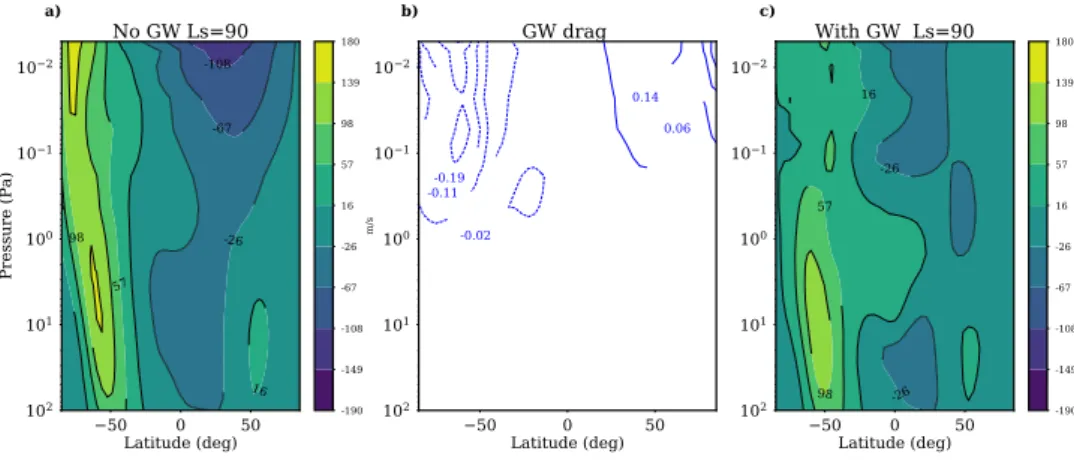
50 0 50 Latitude (deg) 102 101 100 101 102 Pressure (Pa) a) -108 -67 -26 16 16 57 98 No GW Ls=90 -190 -149 -108 -67 -26 16 57 98 139 180 m/s 50 0 50 Latitude (deg) 102 101 100 101 102 b) -0.19 -0.11 -0.02 0.06 0.14 GW drag 50 0 50 Latitude (deg) 102 101 100 101 102 c) -26 -26 16 57 98 With GW Ls=90 -190 -149 -108 -67 -26 16 57 98 139 180 m/s

Figure 2. Same as Figure 1 but for early northern hemisphere summer Ls=90◦

with the one estimated by Parish et al. [2009] and with the lower limit estimated by Fritts

et al.[2006]). Nevertheless, a quantitative comparison of GW-induced wind drag should

be taken with caution, because it would require first a detailed inter-comparative study be-tween the two different GW parameterizations, which is not straightforward and should be addressed in a future dedicated paper. Here we have investigated the possible impact of the vertical resolution on the GW drag by increasing the vertical resolution from 6-7 km (32 lev-els) to 2-3 km (54 levlev-els). The results (see Figure in Supplement Material) show that GW drag values are of the same order of magnitude with higher resolution than with our standard GCM model resolution, confirming that our GW parameterization does not depend on the vertical resolution."

5.1 Comparison with wind observations

As shown in the previous section, the non-orographic GW parameterization imple-mented in this work produces major changes on the simulated zonal winds. Overall, the GW slow down zonal winds everywhere, and in the tropics they become nearly zero (panels c

50 0 50 Latitude (deg) 102 101 100 101 102 Pressure (Pa) a) -67 -26 16 16 57 57 98 139 No GW Ls=210 -190 -149 -108 -67 -26 16 57 98 139 180 m/s 50 0 50 Latitude (deg) 102 101 100 101 102 b) -0.52 -0.38 -0.23 -0.08 0.06 GW drag 50 0 50 Latitude (deg) 102 101 100 101 102 c) -67 -26 16 57 98 With GW Ls=210 -190 -149 -108 -67 -26 16 57 98 139 180 m/s

Figure 3. Same as Figure 1 but for early northern hemisphere fall Ls=210◦

50 0 50 Latitude (deg) 102 101 100 101 102 Pressure (Pa) a) -190 -149 -108 -67 -26 16 16 57 98 No GW Ls=270 -190 -149 -108 -67 -26 16 57 98 139 180 m/s 50 0 50 Latitude (deg) 102 101 100 101 102 b) -0.78 -0.42 -0.06 0.31 0.67 GW drag 50 0 50 Latitude (deg) 102 101 100 101 102 c) -26 -26 16 16 57 98 With GW Ls=270 -190 -149 -108 -67 -26 16 57 98 139 180 m/s

Figure 4. Same as Figure 1 but for early northern hemisphere winter Ls=270◦. The white spot in panel a) represents values lower than -190 m/s.

in Figures 1-2). Unfortunately, there are no direct wind observations to compare with, ex-cept for rare and sparse observations from ground based telescopes [Sonnabend et al., 2012;

Lopez-Valverde et al., 2016]. The wind fields derived from MCS temperature fields using

geostrophic balance are based on several assumptions (see McCleese et al. [2010]) and they are certainly not the gold standard to validate model simulations. They are estimates of zonal gradient wind calculated via thermal wind, but we can expect the atmosphere of Mars to be more complicated than that. Here instead we compare our results with the retrieved wind velocity in the mesosphere of Mars during one observing campaign occurred in MY29 (cam-paign B, in November and December 2007 described in Sonnabend et al. [2012].) Figure 5 shows extracted simulated daytime zonal mean wind values for the corresponding seasons (Ls=0-30◦and Ls=330-360◦), latitudes and altitude range. MGCM wind were averaged be-tween 50 and 116 km, according to the contribution function of the measurements. The re-sults of Sonnabend et al. [2012] (their Figure 8) are also plotted in Figure 5. When compar-ing the results, there are several discrepancies between model and data, particularly in the equatorial region (30◦N-30◦S), where the inclusion of the GW scheme does not seem to im-prove the wind values. MGCM averaged field without the non-orographic GW are retrograde near the equator, with values within the error bars of most of the measured values, while the results extracted from the MGCM after the implementation of the GW scheme are close to zero. The only exception is the measurement around the equator (latitude = 11◦N) showing

120

90

60

30

0

30

60

90

120 150 180 210

75

50

25

0

25

50

75

Latitude

MY29 Ls= 0-30

Sonnabend et al. 2012 (Campaign B) MGCM with GW

MGCM No GW

120

90

60

30

0

30

60

90

120 150 180 210

Eastward zonal wind [m/s]

75

50

25

0

25

50

75

Latitude

MY29 Ls= 330-360

Sonnabend et al. 2012 (Campaign B) MGCM with GW

MGCM no GW

Figure 5. Comparison of retrieved wind values as in Sonnabend et al. [2012] (see their Figure 8) indicated with stars, with predicted daytime values from the LMD-MGCM with the non-orographic GW scheme on (green triangles) and off (red dots). The comparison is given for campaign B occurred during two martian

months of MY29: Ls=0-30◦(upper panel) and Ls=330-360◦(bottom panel). The wind values from the

MGCM were averaged between 50 and 100 km (top of the model), according to the contribution function described in Sonnabend et al. [2012]. The error plotted for the MGCM dataset is the full month standard deviation at the exact latitudes of the measurements.

zonal wind ± 30 m/s, where a MGCM with zero wind in that region is consistent. The same is true for the campaign A occurred in MY30 (not shown here), where low westerlies winds around 20-30 m/s at southern latitudes are also consistent with values simulated in this work. In northern latitudes the fit is not very good (both with or without GW) but there the data is also all over the place, with 30 m/s westward in campaign A and 180 m/s eastward in cam-paign B, at a similar season, and measured uncertainties are also larger.

5.2 Impact of GW mean flow forcing parameters

The momentum deposited by GW on the mean state not only may reverse easterly sol-sticial equatorial zonal jets in the middle atmosphere (∼ 5-0.05 Pa) and weaken the

west-10

10

Pressure (Pa)

-60

-20 20

20

60

60

100

Zonal Wind (No GW)

-180 -140 -100 -60 -20 20 60 100 140 180 m/s

10

10

134

149

149

149

149

163

163

163

178

192207

207

Temperature (No GW)

10

10

Pressure (Pa)

GW drag on zonal wind

-0.30 -0.25 -0.20 -0.15 -0.10 -0.05 0.05 0.10 m/s/sol

10

10

-8

-3

-3

3

3

3

3

3

8

8

14

14

19

19

Temperature diff. (GW - NO GW)

50

0

50

Latitude (deg)

10

10

Pressure (Pa)

-95

_-68

_-41

_-41

-68

-14

-14

14

41

6895

Zonal Wind diff. (GW - NO GW)

-150 -123 -95 -68 -41 -14 14 41 68 95 123 150 m/s

50

0

50

Latitude (deg)

10

10

-14

-14

-8

-8

-8

-3

-3

3

38

8

14

Meridional Wind diff. (GW - No GW)

-25.00 -19.44 -13.89 -8.33 -2.78 2.78 8.33 13.89 19.44 25.00 m/s

Figure 6. Mean zonal wind in m/s (panel a) and temperature (panel b) simulated by the MGCM before

the implementation of the non-orographic GW parameterization in the period Ls= 0-30◦. Panel c shows the

mean GW drag on the zonal wind in m/s/sol when the non-orographic GW scheme is on: negative values indicate deceleration of zonal wind and positive field is acceleration. Only values above |0.001| m/s/sol have been plotted. Panels d, e and f represent the simulated difference "With GW - Without GW" of temperature field in K, zonal winds in m/s, and meridional winds in m/s, respectively.

10

10

Pressure (Pa)

_-140

-100

-60

-20

20

60

100

Zonal Wind (No GW)

-180 -140 -100 -60 -20 20 60 100 140 180 m/s

10

10

134

134

149

149

163

163

178192207

₂₂₁

Temperature (No GW)

10

10

Pressure (Pa)

GW drag on zonal wind

-0.43 -0.35 -0.27 -0.20 -0.12 -0.04 0.04 0.12 0.20 m/s/sol

10

10

-8

-8

-3

-3

-3

-3

3

3

3

8

8

Temperature diff. (GW - No GW)

50

0

50

Latitude (deg)

10

10

Pressure (Pa)

-41

-14

14

41

68

68

95

95

Zonal Wind diff. (GW - NO GW)

-150 -123 -95 -68 -41 -14 14 41 68 95 123 150 m/s

50

0

50

Latitude (deg)

10

10

-8

-8

-3

-3

-3

3

3

3

8

8

14

19

Meridional Wind diff. (GW - No GW)

-25.00 -19.44 -13.89 -8.33 -2.78 2.78 8.33 13.89 19.44 25.00 m/s

10

10

Pressure (Pa)

-180

-140

-100

-60

-20

20

60

100

140

Zonal Wind (No GW)

-180 -140 -100 -60 -20 20 60 100 140 180 m/s

10

10

134

149

149

163

163

178

178

192

192207

221

236236

Temperature (No GW)

10

10

Pressure (Pa)

GW drag on zonal wind

-2.00 -1.62 -1.25 -0.88 -0.50 -0.12 0.25 0.62 1.00 m/s/sol

10

10

-19

-14

-14

-8

-8

-3

-3

-3

-3

3

3

3

3

8

8

8

8

8

Temperature diff. (GW - NO GW)

50

0

50

Latitude (deg)

10

10

Pressure (Pa)

-68

-41

-14

-14

14

41

₆₈

95

123

123

150

Zonal Wind diff. (GW - NO GW)

-150 -123 -95 -68 -41 -14 14 41 68 95 123 150 m/s

50

0

50

Latitude (deg)

10

10

_-14

_-25

_-19

-14

-14

-8

-8

-8

-3

-3

3

3

3

8

8

8

14

19

25

Meridional Wind diff. (GW - No GW)

-25.00 -19.44 -13.89 -8.33 -2.78 2.78 8.33 13.89 19.44 25.00 m/s

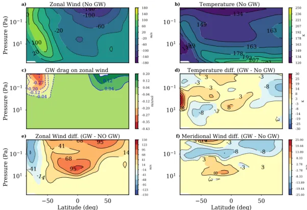
erly zonal jets at mid-high altitudes, as described in section 5, but it also drives changes in the meridional flow. Figures 6, 7, 8 show the alteration of zonal wind, meridional circu-lation and temperature due to parameterized GWs, and the GW drag on zonal wind for the northern hemisphere (NH) Spring (Ls=0,30◦) , NH summer (Ls=90◦,120◦) and NH Winter (Ls=270◦,300◦), respectively. Note that the contour maps in panels c of Figures 6-8 represent monthly averaged GW drag, while Figures 1, 2 and 4, show daily averaged at the correspond-ing solar longitude Ls= 0◦, Ls = 90◦and Ls= 270◦, respectively. Also note that the contour scales are different from Figures 1-4.

Focusing on Figure 6, the equator-to-pole flow increases by ten m/s at about 0.5 Pa (60 km approximately) with respect to the runs without GW (see panel f), thus increasing conver-gence at the pole, hence downward motions. As a consequence, the polar warming increases up to 30 K in both hemispheres, and the adiabatic cooling increase up to 10 K in the layers above, at mid-latitudes. At the equator, local heating above 10−1Pa (around 80 km) results from the reduction of ascending branch of the Hadley cell at these altitudes. For the period Ls=90◦,120◦(Figure 7), the dynamical mechanism is analogous, but the impact is smaller: the southern polar warming is increased by more than 15 K, caused by the GW induced ac-celeration of the north-to-south pole meridional flow above 1 Pa (see panel f). Similarly, in the NH winter (Figure 8) the effect of GW is to accelerate the upper branch of the solsti-cial Hadley cell up to 30 m/s, and adiabatic heating takes place due to the intensification of poleward circulation cells, thus increasing the northern polar warming in the middle atmo-sphere of Mars by about 15 K on average. GW drag reaches magnitudes of the order of 1 m/s/sol above 10−2_{Pa in the NH winter solstice (panel b in Figure 2), and produces a major} change in the zonal wind field (∼ 100 m/s), while the impact on the temperature field is rel-atively moderate (∼ 10-20 K). Those considerations indicate that GW induced alteration of the meridional flow is responsible for the simulated temperature variation. The impact on the temperature field will be also discussed in the next session.

6 Results: comparison with MCS data

Since the characteristics of GW spectrum are not well known on Mars, the strategy adopted in this work was to identify a set of reference tunable GW parameters that reduced model data biases by the greatest amount by comparing the LMD-MGCM and MCS thermal structure, specifically using diurnal tides as diagnostics. We run 26 simulations of a full Mar-tian Year (MY 29) with non-orographic GW parameterization included. The subset of "best-fit" GW characteristics listed in Table 1 was selected with the help of sensitivity tests (see Section 7). Both MCS data and LMD-MGCM simulations were binned in boxes of 3.75◦ latitude x 5.625◦longitude.

In this section we will focus only on the LMD-MGCM simulations performed with the non-orographic GW scheme activated using the wave characteristics as in Table 1. Note that they correspond to Case 2 in Table 2.

c kh F0 Sc

[m/s] [km] kg m−1s−2

[1 - 30] [10 - 300] [0 - 7 · 10−7_{] 1}

Table 1. Best-fit wave characteristics in the GW scheme implemented in this work: c the absolute phase

speed, k_hthe horizontal wavelength amplitude, F0the vertical momentum (EP-flux) at the source and Scthe

saturation parameter. Values in the bracket indicate the extremes of the probability distribution used here for the reference simulations.

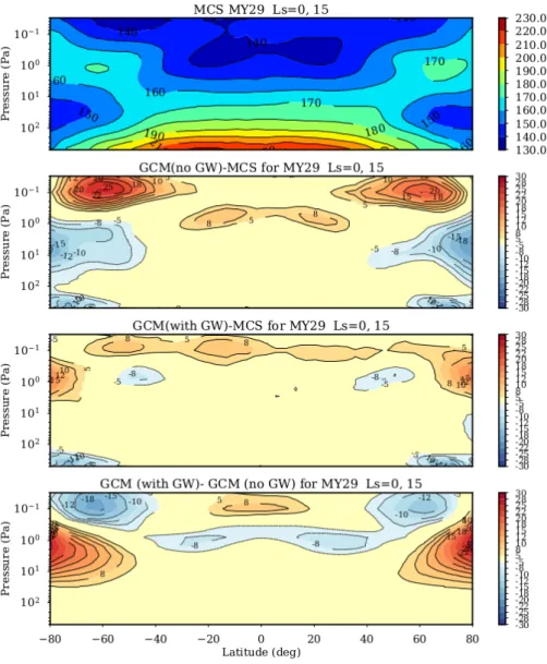
Figure 9. Data-model comparison of zonal mean day-night temperature (Tam+ Tpm)/2 averaged over

the NH Spring Equinox (Ls=0◦-15◦) for MY29. Measurements by MCS/MRO are in top panel. Differences

MGCM-MCS without and with non-orographic GW parameterization are shown in the second and third pan-els from the top, respectively. The bottom panel shows temperature differences between model simulations (with GW - without GW).

Figure 11. As in Figure 9 but for NH summer solstice (Ls=90◦-105◦). Note that the white spot at equato-rial latitudes near the surface is due to the topography.

6.1 Impact of non-orographic GW drag on LMD-MGCM thermal structure Examples of the impact of our GW scheme on the thermal structure of the Martian mesosphere predicted by the LMD-MGCM (up to about 100 km) are given in Figures 9-18. Figures 9-13 compare zonal mean day-night temperature averages Tmeanfrom MCS data (top panels) with model results from the LMD-MGCM with and without the non-orographic GW parameterization (middle panels). Differences between the model runs with and without the parameterization are also given. Tmeanstands for (Tam+ Tpm)/2, where Tamand Tpm are the temperature at 03:00 h and 15:00 h local time, respectively. As discussed in Section 4, latitudes larger than 80◦(North and South) are excluded from this study to avoid compar-ison at non-homogeneous local time. In Figures 17 and 18 we plot examples of nightime (Tam) and daytime (Tpm) zonal mean temperatures at pressure z= 1 Pa, for latitude ranges 20◦S-20◦N and 60◦N-80◦N, respectively, during MY29 and for all seasons in which MCS data are available (Ls= 0-330◦).

It is assumed that the state of the model before including the new GW parameteriza-tion was consistent but incomplete to represent the reality, and we add the new GW parame-terization hoping to get a more realistic emulation of the Martian atmosphere by our GCM. However, there is a chance that the new parameterization is instead compensating for errors in other routines. This weakness applies to any GCM study and we have to make the underly-ing assumption that there is no unphysical error in the existunderly-ing physics routines implemented in our model. Notably, the parameterization by Madeleine et al. [2014] and Navarro et al. [2014] indeed improved the comparison between the LMD-MGCM and the observations for good physical reasons (e.g. coupled dynamical-radiative processes for dust, and radia-tive effect of clouds), but we have no choice other than to conduct our GCM work under the above-mentioned underlying assumption.

6.1.1 Equinoxes

The general circulation at the Mars equinoxes is dominated by two prograde mid-latitude jets corresponding to the equator-to-pole heating gradients at low altitude with a single Hadley cell in each hemisphere. Above 10 Pa (∼ 40 km), the LMD-MGCM predicts a dynamically driven temperature inversion around 1 Pa (∼ 60-70 km) above both poles

[For-get et al., 1999]. When the GW scheme is off, we found that during the Northern Hemisphere

(NH) Spring Equinox (see Figure 9) the MGCM-MCS difference exceeds 20 K; in particu-lar the model is colder at middle to high latitudes below 1 Pa, and warmer in the region be-tween 1 and 0.1 Pa (about 50-75 km altitudes), mainly around 60◦_{latitude (North/South).} In the MGCM version with the non-orographic GW scheme on, the region between 50◦_and 80◦_{latitude (North/South) is up to 22 K warmer below 1 Pa and cooler above between 40}◦ and 70◦latitude (North/South), thus reducing the differences with MCS data. The bottom panel in Figure 9 illustrates the net effect of our non-orographic GW parameterization on zonal mean average temperature. Temperature in the tropical region (40◦S-40◦N) is also re-duced by about 8 K around 1 Pa, in better agreement with the data. Similar conclusions hold when comparing results for NH Autumn (Figure 10). However, in this case the warmer re-gion around 1 Pa around the equator is only partially reduced when the non-orographic GW scheme is activated. In Figures 9 and 10, the impact of GW on the temperature field is the one described for orographic (i.e. low phase speed) GW on Mars by early modeling stud-ies like Barnes [1990]; Collins et al. [1997]; Forget et al. [1999]: the adiabatic cooling at low latitudes and the polar warming is enhanced and shifted to lower altitudes (10 to 100 Pa level) as a results of the GW friction acting on the zonal wind. Lowering the zonal wind reduces the Coriolis forces that limit the poleward meridional winds. In particular, this en-hances the mass convergence at high latitudes and strengthens the polar warming.

6.1.2 Solstices

Concerning the solstice, the impact of non-orographic GW in MGCM simulations is also significant, during both the NH summer solstice (Ls=90◦-105◦) and NH winter (Ls=270◦

-285◦), as shown in Figure 11 and 12, respectively. As discussed in Forget et al. [1999], around Northern winter solstice the strong pole-to-pole diabatic forcing creates a quasi-global Hadley cell which extends to 0.05 Pa (∼ 80 km). In such a cell the Coriolis force contributes to ac-celerate the poleward meridional motion on Mars, thus inducing a mass convergence and strong warming of the middle polar atmosphere down to about 5 Pa (∼ 25 km), as also ob-served [Jakosky and Martin, 1987; Theodore et al., 1993]. Forget et al. [1999] suggested that thermal inversions can generally be expected around 1 Pa (60-70 km) above the winter po-lar regions near solstice, and above both poles near equinox. However, we note here that the effect of GW is not an enhancement of high latitude (60◦-80◦) warming (see also Figures 14 and 13), as during the equinoxes. On the contrary, around Northern winter solstice the GW drag tends to reduce the high latitude warming by more than 15 K (e.g. Figure 12), while heating the atmosphere above 1 Pa (∼ 60 km) at low/middle latitudes. This appears different than in most published results on orographic and non-orographic GW, and the opposite of what was simulated at the equinoxes (compare bottom panels in Figures 9 and 12). In reality, as discussed in Section 5.2, the polar warming (poleward of 80◦N, not shown in Figures 12) is increased as expected (see Figure 8), and it is only between 30◦N and 80◦N that the warm-ing is reduced. This results from the poleward shift of the warmwarm-ing subsidence, but also from the direct effect of the GW drag on the meridional wind and on the damping of thermal tides (see section 6.2), which partly controls the high latitude warming around northern winter sol-stice [Wilson and Hamilton, 1996]. Data-model comparison improves mostly in NH winter, with biases at pressure range 10-1 Pa reduced up to 20 K, especially between 40◦_{N and 80}◦_N latitude (see Figure 12). There are still differences between MGCM and MCS results: at sim-ilar pressure levels and around the equator simulations are warmer than MCS data by 5 K, thus increasing model biases. Possible causes for those remaining discrepancies are related to: i) the uncertainties on the dust distribution in the model during the dust season, ii) the ra-diative effects of water-ice clouds on the thermal structure during the NH summer, and/or iii) the vertical resolution in the water ice cloud structure, during the northern summer season. At the aphelion the uncertainties related to the cloud modeling are larger than the effect of non-orographic GW on the large-scale circulation, and it is still challenging to reach a good accuracy to represent it well with GCMs.

6.1.3 Thermal structure seasonal variations

To illustrate the seasonal evolution of simulated temperature after the implementa-tion of the GW scheme into the LMD-MGCM using the baseline GW parameters as in Ta-ble 1, zonal day-night averages (Tam+ Tpm)/2 are plotted in Figures 13-16 as function of solar longitude Lsfor a selection of latitudinal bands: 20◦S-20◦N, 40◦N-60◦N, 60◦N-80◦N and 60◦S-80◦S. Overall, those figures indicate that there is a small reduction in the magni-tude of the biases at most seasons and latimagni-tudes, with some notable exceptions: (i) the mid-altitude negative bias at high southern latitudes in the first half of the year (northern spring and summer) is greatly reduced up to 20 K (Figure 13), (ii) the mid-altitude positive bias at high northern latitudes in early winter (Ls= 240-270) also decreases by 15-20 K (Figure 14). Note that this period corresponds to the bulk of the dust storm season, yet the GW scheme improves the predicted thermal structure at those latitudes (iii) Positive biases in northern mid-latitudes (40◦-60◦N) are generally reduced up to 10 K at all altitudes and times of the year, except at very high altitudes around local winter solstice (Figure 15) (iv) Large neg-ative biases at low altitudes at high latitudes (in northern fall) and northern mid-latitudes (in northern fall and winter) are not improved by the non-orographic GW parameterization and may be due to incorrect dust distributions and/or interactions between dust and water ice clouds during the dustiest time of the year. Remaining biases in the dust storm season (Ls= 180◦-330◦) between GCM simulations with the GW scheme activated and MCS obser-vations can be attributed to aerosol effects. As circulation and vertical transport of dust are intertwined [Kahre et al., 2015], and presence of water ice clouds critically depends on tem-perature, complex feedbacks between modeled temperature and modeled fields of aerosols prevail, that need to be further explored in future model developments.

Figure 13. Zonal mean temperature as in Figures 9-12 but as function of solar longitudes, in the latitudinal band 60◦S-80◦S.

Figure 14. Zonal mean temperature as in Figures 9-12 but as function of solar longitudes, in the latitudinal band 60◦N-80◦N.

Figure 15. Zonal mean temperature as in Figures 9-12 but as function of solar longitudes, in the latitudinal band 40◦N-60◦N.

Figure 16. Zonal mean temperature as in Figures 9-12 but as function of solar longitudes, in the equatorial

0 50 100 150 200 250 300 Ls 120 130 140 150 160 170 180 Temperature (K)

MY29 NIGHT Lat=-20,20 z= 1Pa MGCM with GW MGCM no GW MCS 0 50 100 150 200 250 300 Ls 120 130 140 150 160 170 180 Temperature (K)

MY29 DAY Lat=-20,20 z= 1Pa MGCM with GW MGCM no GW MCS 0 50 100 150 200 250 300 Ls 20 10 0 10 20 Differences (K) 0 50 100 150 200 250 300 Ls 20 10 0 10 20 Differences (K)

Figure 17. Seasonal variation of zonal temperature at pressure 1 Pa at nighttime LT=03:00 (top left) and daytime LT=15:00 (upper right), averaged at equatorial latitudes 20S-20N. MGCM simulations without (blue solid line) and with the GW scheme included (red solid line) using the subset of GW parameters as in Table 1 are shown together with MCS observations (black solid lines). Temperature differences (MCS-MGCM) are plotted in K in the lower panels, for night (bottom left) and day time (bottom right)

0 50 100 150 200 250 300 Ls 140 150 160 170 180 190 200 210 Temperature (K)

MY29 NIGHT Lat=60,80 z= 1Pa MGCM with GW MGCM no GW MCS 0 50 100 150 200 250 300 Ls 140 150 160 170 180 190 200 210 Temperature (K)

MY29 DAY Lat=60,80 z= 1Pa MGCM with GW MGCM no GW MCS 0 50 100 150 200 250 300 Ls 20 10 0 10 20 Differences (K) 0 50 100 150 200 250 300 Ls 20 10 0 10 20 Differences (K)