DOI: 10.1126/science.1167625
, 1714 (2009);
323
Science
et al.
Chris M. Brierley,
Weakened Hadley Circulation in the Early Pliocene
www.sciencemag.org (this information is current as of March 26, 2009 ):
The following resources related to this article are available online at
http://www.sciencemag.org/cgi/content/full/323/5922/1714
version of this article at:
including high-resolution figures, can be found in the online
Updated information and services,
http://www.sciencemag.org/cgi/content/full/1167625/DC1
can be found at:
Supporting Online Material
http://www.sciencemag.org/cgi/content/full/323/5922/1714#otherarticles
, 7 of which can be accessed for free:
cites 27 articles
This article
http://www.sciencemag.org/cgi/collection/atmos
Atmospheric Science
:
subject collections
This article appears in the following
http://www.sciencemag.org/about/permissions.dtl
in whole or in part can be found at:
this article
permission to reproduce
of this article or about obtaining
reprints
Information about obtaining
is a
Science
2009 by the American Association for the Advancement of Science; all rights reserved. The title
Copyright
American Association for the Advancement of Science, 1200 New York Avenue NW, Washington, DC 20005.
(print ISSN 0036-8075; online ISSN 1095-9203) is published weekly, except the last week in December, by the
Science
on March 26, 2009
www.sciencemag.org
JX–X)]2}. We then expect the singlet lifetime
lengthening to be on the order of [(JA–A– JX–X)/
(J – J′)]2. However, the importance of discon-nected eigenstates was apparently not appreciated, in part because, in the absence of hyperpolar-ization and a mechanism to populate the state, the associated state has no obvious applications.
The perturbation calculation is easily extended to diacetyl, where the ratio (J T J′)/(JA–A– JX–X) is also small (the minus sign gives the larger value in cases such as ours, where the couplings have op-posite signs). Although the spectra in Fig. 4, C and F, are quite complex, assuming the couplings have the same value as in the hydrate (which gives the excellent spectral fit in Fig. 4F) shows that the over-lap of the singlet state with an eigenstate is better than 0.96. This result is also readily verified by pre-cise numerical analysis of this eight-spin system, and thus we predict more than an order-of-magnitude lengthening of the spin lifetime. In effect, the strong coupling between the two carbons quenches com-munication with other spins—virtually all the spectral complexity comes from the other three carbon states, and singlet-to-triplet interconversion is slow. Of course, perdeuteration dramatically reduces even this limited singlet-triplet mixing and further in-creases the lifetime.
The advantage of the perturbation theory cal-culation is that it lets us discuss the generic case. The generalization is more subtle than one might expect. The common case of magnetic equivalence [where the two spins have the same resonance fre-quency and each of the two spins is coupled iden-tically to every other spin (12)] does not necessarily produce a disconnected eigenstate. For example, any two of the spins in a freely rotating methyl group are magnetically equivalent, but the energy level diagram for three equivalent spins produces no fully disconnected states, so the immunity to envi-ronmental perturbations is not present. The only possible disconnected eigenstate for two spins is the singlet; for a larger even number of spins with enough symmetry [e.g., benzene (29)] other dis-connected states exist, although they might be difficult to access in practice.
The critical constraint for producing a discon-nected eigenstate is that the coupling between two spins substantially exceeds both the couplings to other spins and the resonance frequency differ-ence between the spins. Systems of interest as hy-perpolarized contrast agents have two nearby H,
13
C,15N,19F, or31P atoms that satisfy this con-straint. They have a precursor where the two atoms are inequivalent (hence permitting hyperpolariza-tion of thea1b2population), which can be converted
to the contrast agent by chemical manipulation in a time that is short compared with the normalT1.
Finally, they have a biological pathway that again makes them inequivalent, permitting detection of the hyperpolarization. Diacetyl in vivo satisfies these conditions. Partition in vivo between hydro-phobic and hydrophilic phases would modulate the exchange rate (drastically reducing the water centration and, hence, lengthening the time to con-vert from singlet); even ignoring hydration, the first
metabolite is acetoin with inequivalent carbons. More generally, the simplest case is two equivalent adjacent carbons or nitrogens without directly bonded hydrogens, as in diacetyl, naphthalene, and oxolin (an antiviral compound) or in many derivatives of pyridazine or phthalazine, which have recently been shown to have vascular endothelial growth factor receptor–2 inhibitory activity (30). In other cases, deuteration can essentially eliminate the coupling to outside nuclei, as could very weak irradiation (far less than is necessary when the spin systems differ in their chemical shift frequency). At moderate fields, even molecules with not-quite-equivalent spins (such as the 3,4-13C versions ofL-dopa or dopa-mine) might be usable, as the degradation pathway leads to compounds such as HVA with substantial asymmetry.
References and Notes
1. J. R. MacFall et al., Radiology 200, 553 (1996). 2. C. R. Bowers, D. P. Weitekamp, J. Am. Chem. Soc. 109,
5541 (1987).
3. J. Natterer, J. Bargon, 31, 293 (1997).
4. K. Golman et al., Magn. Reson. Med. 46, 1 (2001). 5. A. Abragam, M. Goldman, Rep. Prog. Phys. 41, 395 (1978). 6. K. Golman, J. H. Ardenkjaer-Larsen, J. S. Petersson,
S. Mansson, I. Leunbach, Proc. Natl. Acad. Sci. U.S.A. 100, 10435 (2003).
7. D. A. Hall et al., Science 276, 930 (1997). 8. J. Kurhanewicz, R. Bok, S. J. Nelson, D. B. Vigneron,
J. Nucl. Med. 49, 341 (2008).
9. K. Golman et al., Cancer Res. 66, 10855 (2006). 10. M. E. Merritt et al., Proc. Natl. Acad. Sci. U.S.A. 104,
19773 (2007).
11. I. J. Day, J. C. Mitchell, M. J. Snowden, A. L. Davis, Magn. Reson. Chem. 45, 1018 (2007).
12. C. Gabellieri et al., J. Am. Chem. Soc. 130, 4598 (2008). 13. E. R. McCarney, B. L. Armstrong, M. D. Lingwood,
S. Han, Proc. Natl. Acad. Sci. U.S.A. 104, 1754 (2007).
14. The nomenclature used here is explained more fully, with specific examples, in textbooks such as (15). 15. E. D. Becker, High Resolution NMR: Theory and Chemical
Applications (Academic, San Diego, 2000), pp. 171–175. 16. M. Carravetta, O. G. Johannessen, M. H. Levitt,
Phys. Rev. Lett. 92, 153003 (2004).
17. M. Carravetta, M. H. Levitt, J. Chem. Phys. 122, 214505 (2005).
18. P. Ahuja, R. Sarkar, P. R. Vasos, G. Bodenhausen, J. Chem. Phys. 127, 134112 (2007).
19. G. del Campo, M. C. Carmen Lajo, Analyst (London) 117, 1343 (1992).
20. See http://seattlepi.nwsource.com/dayart/20071221/ DiacetylProducts2.pdf for a study done by the Seattle Post-Intelligencer in December 2007.
21. F. G. B. G. J. van Rooy, Am. J. Respir. Crit. Care Med. 176, 498 (2007).
22. R. P. Bell, Adv. Phys. Org. Chem. 4, 1 (1966) and references therein.
23. W. H. Hoecker, B. W. Hammer, J. Dairy Sci. 25, 175 (1942).
24. J. A˚. Jakobsen et al., Eur. Radiol. 15, 941 (2005). 25. R. J. Abraham, H. J. Bernstein, Can. J. Chem. 39, 216
(1961).
26. F. A. L. Anet, Can. J. Chem. 39, 2262 (1961). 27. J. I. Musher, E. J. Corey, Tetrahedron 18, 791 (1962). 28. J. A. Pople, W. G. Schneider, H. J. Bernstein, Can. J. Chem.
35, 1060 (1957).
29. A. Saupe, Z. Naturforsch. 20a, 572 (1965). 30. A. S. Kiselyov, V. V. Semenov, D. Milligan, Chem. Biol.
Drug Des. 68, 308 (2006).
31. This work was supported by the NIH under grant EB02122 and by the North Carolina Biotechnology Center. We thank D. Bhattacharyya for his help in determining optimal conditions to hyperpolarize diacetyl; M. Jenista for help with calculations; T. Ribiero for his assistance in running NMR spectra; L. Bouchard for discussions of singlet character in strongly coupled systems; and S. Craig, E. Toone, D. Coltart, and M. S. Warren for particularly useful discussions on the chemistry of these compounds. A provisional patent has been submitted on this work by W.S.W. and Duke University. 27 October 2008; accepted 2 February 2009
10.1126/science.1167693
Greatly Expanded Tropical Warm Pool
and Weakened Hadley Circulation
in the Early Pliocene
Chris M. Brierley,1* Alexey V. Fedorov,1*† Zhonghui Liu,2* Timothy D. Herbert,3
Kira T. Lawrence,4Jonathan P. LaRiviere5
The Pliocene warm interval has been difficult to explain. We reconstructed the latitudinal distribution of sea surface temperature around 4 million years ago, during the early Pliocene. Our reconstruction shows that the meridional temperature gradient between the equator and subtropics was greatly reduced, implying a vast poleward expansion of the ocean tropical warm pool. Corroborating evidence indicates that the Pacific temperature contrast between the equator and 32°N has evolved from ~2°C 4 million years ago to ~8°C today. The meridional warm pool expansion evidently had enormous impacts on the Pliocene climate, including a slowdown of the atmospheric Hadley circulation and El Niño–like conditions in the equatorial region. Ultimately, sustaining a climate state with weak tropical sea surface temperature gradients may require additional mechanisms of ocean heat uptake (such as enhanced ocean vertical mixing).
T
he early Pliocene [~5 to 3 million years ago (Ma)] is often considered the closest analog to the effects of contemporary global warming on Earth’s climate. Indeed, the external factors that control the climate system— the intensity of sunlight incident on Earth’s surface,global geography (1, 2), and, most important, the atmospheric concentration of CO2 (3)—were
similar to present-day conditions. However, high latitudes were warmer, continental ice sheets were largely absent from the Northern Hemisphere, and the sea level was ~25 m higher than today (4, 5).
on March 26, 2009
www.sciencemag.org
The climate of the tropics was also quite different. The sea surface temperature (SST) contrast between the eastern and western equatorial Pacific was very small, and cold surface waters were almost absent from coastal upwelling zones off the western coasts of Africa and the Americas (6–10). These climate conditions are often called a“permanent El Niño” or permanent El Niño–like state (11). This term describes the long-term mean state of the ocean-atmosphere system. In contrast, the modern, intermittent El Niño is the warm phase of a quasi-periodic climate os-cillation, which affects weather and climate patterns worldwide every 4 to 5 years (12, 13). Interannual climate variability may have also existed in the Plio-cene (14), but only during times when the equatorial SST gradient exceeded some critical value (12).
This study focuses on the meridional distribu-tion of SST and its effects on the early Pliocene climate. Understanding changes in this distribu-tion, including variations in the meridional extent of the ocean tropical warm pool, is essential for un-derstanding mechanisms responsible for the gradual transition from the warmer Pliocene to the cooler Pleistocene. It has been hypothesized that the early Pliocene had a relatively deep ocean thermocline in the tropics and that the subsequent shoaling of the thermocline signaled the transition to a colder cli-mate (6). A reduced meridional gradient is required to sustain a deeper tropical thermocline (see below). We first examined the evolution of the merid-ional SST gradient over the past 4 million years in the eastern tropical Pacific (Fig. 1, A and C). We used orbitally resolved records from two Ocean Drilling Program (ODP) sites: Site 1012 (32°N, 118°W) from the California margin, and Site 846 (3°S, 91°W) from the eastern Pacific cold tongue just south of the equator (Fig. 1B). Both data sets are based on alkenone-derived estimates of SST (15). The new data from ODP Site 1012 agree overall with previously published results from ODP Site 1014 (8); however, the present data set has much higher resolution, allowing precise temporal align-ment of equatorial and subtropical records.
According to these data, the mean temperature contrast between the two sites evolved from a very small value of ~2°C at 4 Ma to 7°C by 2 Ma, and then remained fairly constant at nearly present-day levels (Fig. 1C). Superimposed on the gradual trends at each site are Milankovitch cycles driven by variations in Earth’s orbital parameters (1). On orbital time scales, these cycles can produce changes in the SST contrast between the two sites as large as the underlying long-term trends.
The temporal development of the zonal SST gradient along the equator (7) generally mirrors that
of the meridional SST gradient in the eastern Pacific (Fig. 1D), suggesting a strong link between extra-tropical and extra-tropical ocean conditions. The zonal SST gradient reaching its modern value later in the record indicates that meridional temperature changes precondition zonal changes along the equator.
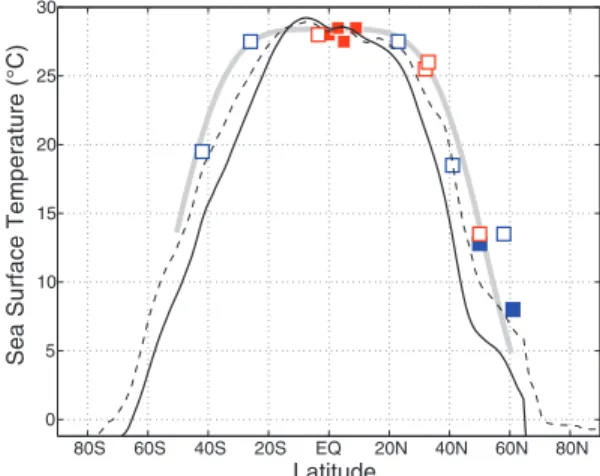
To show that the strong reduction in the merid-ional temperature gradient in the early Pliocene is a robust result, we reconstructed the meridional SST distribution in the mid-Pacific roughly along the dateline (Fig. 2). The period of this reconstruction is ~4 to 4.2 Ma, sometimes called the Pliocene thermal optimum (16). This period coincides with an almost complete collapse of the east-west temperature gra-dient along the equator (6–8) (Fig. 1D); it also fol-lows the closure of the Central America Seaway (2) but precedes climate cooling and the development of large Northern Hemisphere ice sheets (1).
The data in Fig. 2 are based on alkenone and Mg/Ca temperature proxies. Alkenone-derived records for ODP Sites 982, 1012, and 1090 and for Deep Sea Drilling Project Site 607 were produced specifically for this study; the original
temperature records for other sites were published elsewhere (6–10, 17–21). Adjustments were ap-plied to some of the SST data to represent the mid-Pacific in the early Pliocene (15). For example, when using temperatures from the Atlantic to re-construct Pacific SSTs, one must consider that temperatures in the North Atlantic are typically 2° to 7°C higher than in the North Pacific; when using SSTs from the eastern boundary of the basin to re-construct temperatures in the mid-Pacific, one should correct for the effect of coastal upwelling. The over-all temperature distribution in Fig. 2 is robust and does not depend on any individual data point.
Our analysis indicates a considerably warmer Pacific climate in the early Pliocene than that de-termined by the PRISM project in its mid-Pliocene SST reconstructions (5, 22, 23). Furthermore, a strong reduction in the SST gradient from the equator to the subtropics described in our study implies a vast poleward expansion of the ocean low-latitude warm pool (fig. S1), whereas the max-imum tropical temperatures remained close to present-day values (28° to 29°C).
1
Department of Geology and Geophysics, Yale University, New Haven, CT 06520, USA.2Department of Earth Sciences,
University of Hong Kong, Hong Kong, PRC.3Department of
Geological Sciences, Brown University, Providence, RI 02912, USA. 4Geology and Environmental Geosciences, Lafayette College, Easton, PA 18042, USA.5Ocean Sciences, University
of California, Santa Cruz, CA 95064, USA. *These authors contributed equally to this work. †To whom correspondence should be addressed. E-mail: [email protected]
Fig. 1. (A) The evolution of SSTs, as derived from alkenones (15), in two locations: ODP Site 1012 (blue) off the coast of California (32°N, 118°W) and ODP Site 846 (red) in the eastern Pacific just south of the equator (3°S, 91°W). Note the cooling trends over the past 4 million years, shown here as 400,000-year running means (black lines). (B) Locations of the sites in (A). (C) SST difference between the two locations in (B). The meridional SST gradient is minimal at ~4 Ma (2°C) and then increases gradually to modern values (~7.5°C). (D) The zonal SST gradient along the equator (7) from Mg/Ca paleothermometry between ODP Site 806 in the western equatorial Pacific (0°N, 159°E) and ODP Site 847 in the eastern equatorial Pacific (0°N, 95°W). The strength of this temperature gradient varies from 0° to 2°C between 5 Ma and 2 Ma and then increases gradually to modern values (~5.5°C). (E) Locations of the sites in (D).
on March 26, 2009
www.sciencemag.org
The ocean tropical warm pool (currently con-fined mainly to the western equatorial Pacific) is a critical component of the climate system (24), and changes in its meridional extent can have large implications for climate. In particular, me-ridional expansion of the warm pool provides a crucial mechanism for maintaining permanent El Niño conditions in the equatorial region, because cold water in the modern eastern equatorial Pa-cific is sourced from the subtropical subduction zones. Poleward expansion of the warm pool into the subduction regions would lead to warmer waters upwelling in the eastern equatorial Pacific, a deeper ocean thermocline, and consequently a substantial reduction of the SST gradient along the equator. Apparently, such a climate state prevailed at ~4 Ma (Fig. 1, C and D). Thus, to explain the permanent El Niño conditions during the early Pliocene, it is necessary to understand the merid-ional expansion of the ocean warm pool.
To quantify the atmospheric response to the ex-panded tropical warm pool and reduced meridional temperature gradient, we fit a hypothetical SST profile to the data in Fig. 2, which was then used as a boundary condition for an atmospheric general cir-culation model (GCM) (15). In the absence of reli-able simulations of the Pliocene climate with coupled models, simulations with atmospheric GCMs forced with ocean surface boundary conditions arguably re-main the best way to assess climate conditions. Pre-vious studies of the Pliocene with atmospheric GCMs used either earlier PRISM SST reconstruc-tions (5), which lacked adequate data for the tropics and subtropics, or the modern SST profile taken from the dateline and extended zonally (25).
Our numerical calculations confirm that the SST changes in Fig. 2 strongly affect the global climate and atmospheric circulation. As expected, the lack of an SST gradient along the equator acts to elimi-nate the atmospheric zonal circulation [the Walker cell (13)] (fig. S2). However, if the meridional SST gradient were kept at present-day values as in pre-vious studies, the atmospheric meridional circula-tion [the Hadley cells (26)] would compensate by strengthening substantially (25). In contrast, in cal-culations using our Pliocene SST reconstruction, the Hadley circulation weakens (Fig. 3, A and B).
The Northern Hemisphere branch of the Hadley circulation weakens on average by roughly 30%. During boreal winter, the reduction reaches nearly 40%. The center of the Hadley cell moves northward by ~7°, whereas the cell’s latitudinal extent (26) increases by 3° to 4°. These changes of the Northern Hemisphere circulation are a robust response to changes in meridional SST gradient as evinced by additional sensitivity calculations (table S2). The volume transport of the circulation’s southern branch nearly halves, making the southern Hadley cell even weaker than the northern cell. Whether this is a genuine feature of the early Pliocene climate remains to be seen, because there are only a few SST data points currently available in the Southern Hemisphere. Note that coupled models simulating global warm-ing also show a weakenwarm-ing and poleward expansion of the Hadley circulation. However, those effects
are rather modest—roughly 4% and 1° of latitude, respectively, by the end of the 21st century (26).
In our calculations, the reduced meridional temperature gradient also widens the Intertropical Convergence Zone [ITCZ (13)] and decreases its
precipitation intensity (Fig. 3, C and D). A second, weaker ITCZ develops in the Southern Hemisphere, caused by the use of a completely symmetrical SST profile. The spatial structure of Pliocene precipita-tion indicates that the strongest air uplift occurs over Fig. 2. Estimated distribution of SST
with latitude in the middle of the Pacific (roughly along the dateline) at ~4 Ma. This temperature reconstruction uses data from the Pacific and Indian oceans (red boxes) and adjusted data from the Atlantic (blue boxes). Open boxes indi-cate alkenone-based data; solid boxes indicate Mg/Ca-based data. Thin solid line: SST from the dateline for the modern climate. Dashed line: latest estimates of the mid-Pliocene temper-atures (~3 Ma) along the dateline from the PRISM project (22, 23). Thick gray line: a portion of the hypothetical SST profile used as a boundary condition for numerical simulations. The original data
and the temperature adjustments are given in table S1.
Fig. 3. The meridio-nal overturning stream-function (A and B) and the surface precipita-tion (C and D) simulated with the atmospheric GCM (CAM3). Note the reduction in the strength of the Hadley cells and precipitation intensity over the ocean for the Pliocene simulation.
on March 26, 2009
www.sciencemag.org
orographic features (such as the East African High-lands) rather than over the ocean. Weak SST gradients, and hence a lack of localized wind convergence, over the ocean cause orographic air uplift and ocean-land temperature contrasts to become essential for triggering tropical precipitation.
Terrestrial paleodata provide verification of gross changes in precipitation anticipated over land by our calculations. For example, the model pre-dicts stronger precipitation over southwest and east Africa, the Sahara desert, and Australia, consistent with pollen-based precipitation data (table S3). Comparison of changes over North America is inconclusive because of large error bars in the paleodata (27) and large natural variability in precipitation intensity in that region.
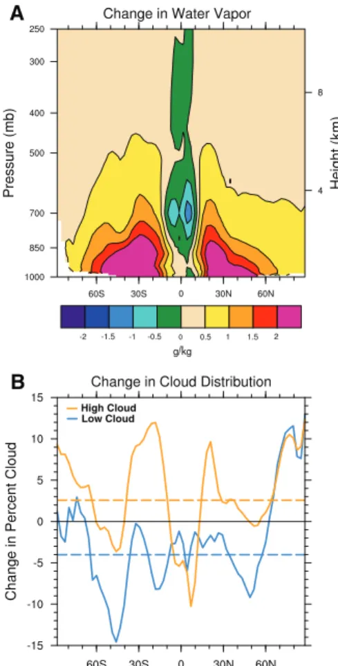
The water vapor content of the atmosphere in-creases significantly (Fig. 4A) as a consequence of the Clausius-Clapeyron relationship (28), despite the substantial reduction in the strength of
atmo-spheric convection over the ITCZ in the Pacific. The increase in water vapor (a potent greenhouse gas) is a major factor in sustaining the warm Plio-cene climate. It causes a reduction of 14.6 W m−2 in outgoing long-wave radiation at the top of the atmosphere (relative to the present); variations in cloud distribution (Fig. 4B) account for a further reduction of 5.6 W m−2. Because the net increase in atmospheric water vapor (by roughly 30%) is large-ly a consequence of the expanded ocean warm pool, a climate model will not be able to capture the full extent of the Pliocene warmth unless it can simulate SST patterns in the tropics and subtropics correctly. Further, our calculations show a slight increase in total poleward heat transport from low to high latitudes (fig. S3). However, the partitioning of the heat transport between the ocean and atmosphere poses the following problem: We find a significant decrease in the heat transport by the atmosphere and an implied increase in ocean heat transport (fig. S3). This result contradicts studies using ocean GCMs with low vertical diffusion, which suggest that a per-manent El Niño should be associated with reduced heat transport by the ocean (29). According to those studies, the ocean typically gains a large amount of heat over the tropical Pacific cold tongue; warmer conditions in that region would entail a reduction in ocean heat uptake there, and hence a smaller ocean heat transport. Attempts to simulate the Pliocene cli-mate with coupled atmosphere-ocean GCMs (14) have not yet succeeded in replicating the collapse of the SST gradient along the equator, presumably because of this issue.
One way to resolve the heat transport problem in such a climate state with weak SST gradients is to allow the ocean to gain heat over a much broader
region of the tropics than just the equatorial cold tongue. This would necessitate a substantial increase in ocean vertical mixing rates (or vertical diffusion), which may result from weaker ocean stratification (20) and/or enhanced mixing of the upper ocean by hurricanes (30). Should such an increase in ocean mixing occur, it would lead to larger heat uptake and greater poleward heat transport by the ocean, even with a weak or absent equatorial cold tongue.
To test this hypothesis, we ran a coupled GCM with elevated atmospheric CO2 concentrations
and vertical diffusion uniformly increased in the upper tropical ocean. Preliminary results with en-hanced mixing produce a mean state much closer to a permanent El Niño (Fig. 5). There is a much greater warming in the eastern equatorial Pacific than in the west, a warming of the upwelling re-gions, and a deeper ocean thermocline. At the same time, interannual variability becomes sub-stantially weaker.
Thus, it may be necessary to incorporate ad-ditional mechanisms for increased ocean heat uptake when simulating the early Pliocene climate and, potentially, the response of the tropics to contem-porary global warming. The enormous impacts of changes in the warm pool (such as shifts in global precipitation patterns and cloud cover), as well as tentative evidence that the tropical belt has been expanding poleward over the past few decades (31), make our findings especially relevant to current discussions about global warming.
References and Notes
1. J. Zachos, M. Pagani, L. Sloan, E. Thomas, K. Billups, Science 292, 686 (2001).
2. G. H. Haug, R. Tiedemann, R. Zahn, A. C. Ravelo, Geology 29, 207 (2001).
High Cloud Low Cloud
A
B
Fig. 4. Factors critical for maintaining a warm Pliocene climate. (A) The increase in zonal-mean specific humidity (or water vapor content) from the present day to the early Pliocene (in g/kg). The only reduction in water vapor occurs in a narrow region above the modern ITCZ location, which indicates a weakening of the deep convection in the tropics. (B) Changes in cloud distribution with latitude (solid lines) and their globally averaged values (dashed lines). There is a net increase in cloud fraction for“greenhouse” high clouds and a net decrease for highly reflective low clouds; both effects tend to warm Earth’s surface.
Fig. 5. Difference in ocean temperatures (averaged over the top 250 m) between two greenhouse-warming simulations: a simulation for which we increased the background vertical diffusivity in the upper 400 m of the ocean by an order of magnitude between 40°N and 40°S, and a control simulation. In each case, the CO2concentration was increased instantaneously from preindustrial levels to 355 ppm, and the coupled
model (CCSM3) has been integrated for 180 years (the plot is obtained from a 30-year average at the end of the simulations). A gradual ocean adjustment will continue after 180 years, but we do not expect large qualitative changes in the warming pattern. The actual values of the ocean vertical diffusivity in the Pliocene are highly uncertain, so these experiments serve only to demonstrate the proposed mechanism.
on March 26, 2009
www.sciencemag.org
3. M. E. Raymo, B. Grant, M. Horowitz, G. H. Rau, Mar. Micropaleontol. 27, 313 (1996).
4. H. Dowsett, J. Barron, R. Poore, Mar. Micropaleontol. 27, 13 (1996).
5. A. M. Haywood, P. J. Valdes, B. W. Sellwood, Global Planet. Change 25, 239 (2000).
6. A. V. Fedorov et al., Science 312, 1485 (2006). 7. M. W. Wara, A. C. Ravelo, M. L. Delaney, Science 309,
758 (2005); published online 23 June 2005 (10.1126/science.1112596).
8. P. S. Dekens, A. C. Ravelo, M. D. McCarthy, Paleoceanography 22, PA3211 (2007). 9. J. R. Marlow, C. B. Lange, G. Wefer, A. Rosell-Melé,
Science 290, 2288 (2000).
10. K. T. Lawrence, Z. Liu, T. D. Herbert, Science 312, 79 (2006).
11. P. Molnar, M. A. Cane, Paleoceanography 17, 1021 (2002).
12. A. V. Fedorov, S. G. Philander, Science 288, 1997 (2000).
13. S. G. H. Philander, El Niño, La Niño, and the Southern Oscillation (Academic Press, New York, 1990). 14. A. M. Haywood, P. J. Valdes, V. L. Peck,
Paleoceanography 22, PA1213 (2007). 15. See supporting material on Science Online.
16. A. A. Velichko, I. Spasskaya, in The Physical Geography of Northern Eurasia, M. Shahgedanova, Ed. (Oxford Univ. Press, Oxford, 2002), pp. 36–69.
17. T. D. Herbert, J. D. Schuffert, Proc. ODP Sci. Res. 159T, 17 (1998).
18. G. Bartoli et al., Earth Planet. Sci. Lett. 237, 33 (2005).
19. J. Tian, Earth Planet. Sci. Lett. 252, 72 (2006). 20. G. H. Haug, D. M. Sigman, R. Tiedemann, T. F. Pedersen,
M. Sarnthein, Nature 433, 821 (2005). 21. J. Groeneveld et al., Proc. ODP Sci. Res. 202, 1
(2006).
22. H. J. Dowsett, M. M. Robinson, Philos. Trans. R. Soc. London Ser. A 367, 109 (2009).
23. Data are available from http://geology.er.usgs.gov/ eespteam/prism/prism_data.html.
24. A. C. Clement, R. Seager, G. Murtugudde, J. Clim. 18, 5294 (2005).
25. M. Barreiro, G. Philander, R. Pacanowski, A. V. Fedorov, Clim. Dyn. 26, 349 (2006).
26. J. Lu, G. A. Vecchi, T. Reichler, Geophys. Res. Lett. 34, L06805 (2007).
27. U. Salzmann, A. M. Haywood, D. J. Lunt, P. J. Valdes, D. J. Hill, Glob. Ecol. Biogeogr. 17, 432 (2008). 28. I. M. Held, B. J. Soden, J. Clim. 19, 5686 (2006).
29. S. G. H. Philander, A. V. Fedorov, Paleoceanography 18, 1045 (2003).
30. R. L. Sriver, M. Huber, Nature 447, 577 (2007). 31. D. J. Seidel, Q. Fu, W. J. Randel, T. J. Reichler, Nat.
Geosci. 1, 21 (2008).
32. A.V.F. thanks G. Philander, M. Barreiro, R. Pacanowski, Y. Rosenthal, C. Ravelo, P. deMenocal, P. Dekens, A. Haywood, and C. Wunsch for numerous discussions of this topic. Supported by NSF grant OCE-0550439, U.S. Department of Energy Office of Science grants DE-FG02-06ER64238 and DE-FG02-08ER64590, and a David and Lucile Packard Foundation fellowship (A.V.F.), NSF grant OCE-0623487 (T.D.H.), and a Flint Fellowship at Yale University (Z.L.).
Supporting Online Material
www.sciencemag.org/cgi/content/full/1167625/DC1 SOM Text
Figs. S1 to S3 Tables S1 to S3 References
24 October 2008; accepted 9 February 2009 Published online 26 February 2009; 10.1126/science.1167625
Include this information when citing this paper.
Structure of P-Glycoprotein Reveals a
Molecular Basis for Poly-Specific
Drug Binding
Stephen G. Aller,1Jodie Yu,1Andrew Ward,2Yue Weng,1,4Srinivas Chittaboina,1Rupeng Zhuo,3 Patina M. Harrell,3Yenphuong T. Trinh,3Qinghai Zhang,1Ina L. Urbatsch,3Geoffrey Chang1† P-glycoprotein (P-gp) detoxifies cells by exporting hundreds of chemically unrelated toxins but has been implicated in multidrug resistance (MDR) in the treatment of cancers. Substrate promiscuity is a hallmark of P-gp activity, thus a structural description of poly-specific
drug-binding is important for the rational design of anticancer drugs and MDR inhibitors. The x-ray structure of apo P-gp at 3.8 angstroms reveals an internal cavity of ~6000 angstroms cubed with a 30 angstrom separation of the two nucleotide-binding domains. Two additional P-gp structures with cyclic peptide inhibitors demonstrate distinct drug-binding sites in the internal cavity capable of stereoselectivity that is based on hydrophobic and aromatic interactions. Apo and drug-bound P-gp structures have portals open to the cytoplasm and the inner leaflet of the lipid bilayer for drug entry. The inward-facing conformation represents an initial stage of the transport cycle that is competent for drug binding.
T
he American Cancer Society reported over 12 million new cancer cases and 7.6 million cancer deaths worldwide in 2007 (1). Many cancers fail to respond to chemotherapy by ac-quiring MDR, to which has been attributed the failure of treatment in over 90% of patients with metastatic cancer (2). Although MDR can have several causes, one major form of resistance to chemotherapy has been correlated with thepres-ence of at least three molecular “pumps” that actively transport drugs out of the cell (3). The most prevalent of these MDR transporters is P-gp, a member of the adenosine triphosphate (ATP)–binding cassette (ABC) superfamily (4). P-gp has unusually broad poly-specificity, recog-nizing hundreds of compounds as small as 330 daltons up to 4000 daltons (5, 6). Most P-gp substrates are hydrophobic and partition into the lipid bilayer (7, 8). Thus, P-gp has been likened to a molecular “hydrophobic vacuum cleaner” (9), pulling substrates from the membrane and expelling them to promote MDR.
Although the structures of bacterial ABC im-porters and exim-porters have been established (10–15) and P-gp has been characterized at low resolution by electron microscopy (16, 17), obtaining an x-ray structure of P-gp is of particular interest because of its clinical relevance. We describe the structure of mouse P-gp (ABCB1), which has 87% sequence
identity to human P-gp (fig. S1), in a drug-binding– competent state (18, 19). We also determined cocrystal structures of P-gp in complex with two stereoisomers of cyclic hexapeptide inhibitors, cyclic-tris-(R)-valineselenazole (QZ59-RRR) and cyclic-tris-(S)-valineselenazole (QZ59-SSS), re-vealing a molecular basis for poly-specificity.
Mouse P-gp protein exhibited typical basal adenosine triphosphatase (ATPase) activity that was stimulated by drugs like verapamil and col-chicine (fig. S2A) (20). P-gp recovered from washed crystals retained near-full ATPase activity (fig. S3). Both QZ59 compounds inhibited the verapamil-stimulated ATPase activity in a concentration-dependent manner (fig. S2B). Both stereoisomers inhibited calcein-AM export with median inhibi-tory concentration (IC50) values in the low
micro-molar range (fig. S4) and increasing doses of QZ59 compounds resulted in greater colchicine sensi-tivity in P-gp–overexpressing cells (fig. S5).
The structure of P-gp (Fig. 1) represents a nucleotide-free inward-facing conformation ar-ranged as two “halves” with pseudo two-fold molecular symmetry spanning ~136 Å perpen-dicular to and ~70 Å in the plane of the bilayer. The nucleotide-binding domains (NBDs) are sepa-rated by ~30 Å. The inward-facing conformation, formed from two bundles of six transmembrane helices (TMs 1 to 3, 6, 10, 11 and TMs 4, 5, 7 to 9, 12), results in a large internal cavity open to both the cytoplasm and the inner leaflet. The model was obtained as described in (18) by using experimental electron density maps (figs. S6 and S7 and table S1), verified by multipleFobs– Fcalc
maps (figs. S8 to S10), with the topology con-firmed by (2-hydroxy-5-nitrophenyl)mercury(II) chloride (CMNP)–labeled cysteines (figs. S6, B to D; S7C, and S11, and table S2). Two portals (fig. S12) allow access for entry of hydrophobic molecules directly from the membrane. The por-tals are formed by TMs 4 and 6 and TMs 10 and 12, each of which have smaller side chains that could allow tight packing during NBD
dimeriza-1Department of Molecular Biology, The Scripps Research
Institute, 10550 North Torrey Pines Road, CB105, La Jolla, CA 92037, USA.2Department of Cell Biology, The Scripps
Research Institute, 10550 North Torrey Pines Road, CB105, La Jolla, CA 92037, USA.3Cell Biology and Biochemistry, Texas Tech University Health Sciences Center, 3601 4th Street, Lubbock, TX 79430, USA.4College of Chemistry and
Molecular Sciences, Wuhan University, Wuhan, 430072 P. R. China.
†To whom correspondence should be addressed. E-mail: [email protected]