Theoretical and
experimental investigation of near-field multi-focusing
systems
RUIZHI LIU
Département de génie électrique
Thèse présentée en vue de l’obtention du diplôme de Philosophiæ Doctor Génie électrique
Octobre 2019
Cette thèse intitulée :
Theoretical and
experimental investigation of near-field multi-focusing
systems
présentée par Ruizhi LIU
en vue de l’obtention du diplôme de Philosophiæ Doctor a été dûment acceptée par le jury d’examen constitué de :
Jean-Jacques LAURIN, président
Ke WU, membre et directeur de recherche Julien COHEN-ADAD, membre
DEDICATION
ACKNOWLEDGEMENTS
I would like to show my highest gratitude and appreciation to my advisor, Professor Ke Wu for his patience, motivation, immense knowledge, and the continuous support and guidance of my Ph.D study. It is him who teaches me not only knowledge, but also the way of being a qualified researcher and a person full of creativity. His rigorous altitude towards science and spirit of pursuing excellence always encourages me in my study.
Besides my advisor, I would like to thank Prof. Jean-Jacques Laurin, Prof. Ahmed Kishk, and Prof. Julien Cohen-Adad for serving as my committee members.
In addition, I want to show my appreciation to my colleagues and the staff in Poly-Grames for instrumental support and advice in the development and publication of my research.
I would like to thank my parents for supporting me spiritually throughout writing this dissertation and my life in general. Their love, care and support all along make me a confident and optimistic person. And I wish to give thanks to all my friends for their support and to my girlfriend for the encouragement and understanding throughout this challenging work.
RÉSUMÉ
Dans les systèmes de communication modernes, les fonctionnalités d’efficacité énergétique et d'efficacité du spectre sont mises en évidence, attirant de plus en plus l’attention dans la conception des systèmes et des appareils grâce à la demande croissante en débit de données, densité et nombre de terminaux utilisateurs. La technique multi-faisceaux est une caractéristique essentielle de la conception du réseau d'antennes pour systèmes sans fil, qui peut être utilisée pour prendre en charge plusieurs utilisateurs et plusieurs spots avec une grande efficacité. Dans ce travail de recherche, une série de méthodes de développement d’un réseau d’antennes comportant multi-faisceaux de rayonnement électromagnétique dans sa région de champ proche est proposée et présentée. Les travaux de recherche sur la mise au point multiple en champ proche couvrent le développement d’algorithmes, la conception de composants associés, la discussion sur les propriétés de focalisation et leurs méthodes d’amélioration, ainsi que le développement de fonctions d’exploitation et de scénarios d’application.
Dans ce travail, un certain nombre d’algorithmes de modélisation du réseau d’antennes prenant en compte le modèle de champ proche, la compensation de phase et la stratégie d’optimisation sont développés afin non seulement d’identifier les emplacements spatiaux de multiples points focaux dans la région de champ proche, mais également de formuler le modèle de faisceau à ou autour de ces points focaux. Dans l'essentiel, les algorithmes proposés visent essentiellement à réaliser une mise en forme de motif dans la région de champ proche en mettant un accent particulier sur les aspects de conception tels que l'ajustement de la localisation spatiale des points focaux, la spécification des distributions d'amplitude et de phase et l'attribution de polarisations.
La réalisation pratique est également une partie importante de ce travail qui s'intéresse au développement de réseaux d'antennes multi-focales dans la région du champ proche. Par conséquent, les composants, notamment les réseaux d’antennes et les réseaux d’alimentation correspondants, sont conçus et fabriqués pour démontrer expérimentalement les propriétés et les applications à focalisation multiple de ce travail de recherche, validant ainsi la modélisation et l’analyse théoriques. Les réseaux d'antennes multi-focales sont conçus et des travaux expérimentaux sont effectués dans les bandes de fréquences radio et ondes millimétriques avec de bonnes performances.
Différent d'une région d'antenne à champ lointain, le champ électromagnétique dans une région à champ proche implique simultanément des composantes d'énergie réactive et radiative. Pour étudier plus en détail les propriétés du multi-focus dans la région de champ proche, certains paramètres sont définis en relation avec des propriétés de champ spéciales dans la région de champ proche. En particulier, un facteur de réseau d'antennes en champ proche et une résolution de focalisation sont définis et déployés pour estimer la capacité de focalisation d'un réseau d'antennes linéaire ou plan. Des caractéristiques telles que le décalage de focale et l'isolation de polarisation croisée sont examinées et une approche d'amélioration correspondante est donc proposée.
De plus, la fonction de multi-focus est étendue dans ce travail de recherche. Avec les algorithmes proposés, le réseau d'antennes est capable non seulement de se focaliser sur plusieurs points focaux, mais également d'éclairer de multiples zones dans la région de champ proche. Par conséquent, la technique multi-faisceaux proposée est étendue au développement de schémas de traitement de signaux spatiaux comprenant la combinaison de puissance, le fractionnement de puissance et le déphasage. Des techniques populaires telles que la diversité de polarisation peut également être réalisées spatialement avec les solutions développées. Grâce à cette recherche, un ensemble de systèmes à focalisation multiple impliquant le traitement de signal spatial et la fourniture de puissance sont développés, montrant une application prometteuse dans le développement de systèmes de communication hautement efficaces.
ABSTRACT
In modern communications systems, the features of energy efficiency and spectrum efficiency are highlighted, attracting more and more attention in the design of systems and devices thanks to the requirement of ever-increasing data rate, density and quantity of user terminals. Multi-beam technique is an essential enabling design feature of antenna array for wireless systems, which can be used in support of multiple users and multiple spots with high efficiency. In this research work, a series of methods for developing an antenna array that features multiple electromagnetic beaming focuses in its near-field region are proposed and presented. The research work on near-field multi-focus covers the development of algorithms, design of related components, discussion about the focusing properties and their improvement methods, and the expansion of operating functions and application scenarios.
In this work, a number of modeling algorithms of antenna array considering near-field model, phase compensation, and optimization strategy are developed in order not only to identify the spatial locations of multiple focal points in the near-field region but also to formulate the beam pattern at or around those focal points. In essentials, the proposed algorithms aim at realizing a pattern shaping in the near-field region with particular emphasis on design aspects such as adjustment of the spatial location of focal points, specification of amplitude and phase distributions, and allocation of polarizations.
The practical realization is also an important part of this work with interest in developing multi-focus arrays in the near-field region. Therefore, components including antenna arrays and related feeding networks are designed and fabricated for experimentally demonstrating the multi-focusing properties and applications in this research work, which also validate the theoretical modeling and analysis. The multi-focusing antenna arrays are designed, and experimental work is carried out in both radio-frequency and millimeter-wave bands with good performance.
Different from a far-field region of antennas, the electromagnetic field in a near-field region involves reactive and radiative energy components simultaneously. To further investigate the properties of multi-focus in the near-field region, some parametersare defined in connection with special field properties in the near-field region. In particular, near-field array factor and focusing resolution are defined and deployed for estimating the focusing ability of a linear or planar antenna
array. Features such as focal shift and cross-polarization isolation are investigated, and thus a corresponding improving approach is brought about by the proposed algorithms.
Furthermore, the function of multi-focus is extended in this research work. With the proposed algorithms, the antenna array is capable of not only focusing on multiple focal points but also illuminating multiple areas in the near-field region. Therefore, the proposed multi-beam technique is extended to the development of spatial signal processing schemes, including power combining, power splitting and phase-shifting. Popular techniques such as polarization diversity can also be realized spatially with the developed solutions. Through this research, a set of multi-focusing systems involving spatial signal processing and power delivery are developed, showing a promising application in the development of highly efficient communication systems.
TABLE OF CONTENTS
DEDICATION ... III ACKNOWLEDGEMENTS ... IV RÉSUMÉ ... V ABSTRACT ...VII TABLE OF CONTENTS ... IX LIST OF TABLES ...XII LIST OF FIGURES ... XIII LIST OF SYMBOLS AND ABBREVIATIONS... XXCHAPTER 1 INTRODUCTION ... 1
1.1 Background ... 1
1.2 Research objectives and methodologies ... 5
CHAPTER 2 THEORY OF NEAR-FIELD ARRAY FOR MULTI-FOCUS ... 8
2.1 Antenna near field ... 8
2.1.1 Near field ... 8
2.1.2 Near-field models ... 10
2.2 Near-field multi-focus ... 14
2.3 Focusing properties ... 17
2.3.1 Near-field array factor ... 18
2.3.2 Focusing resolution ... 20
2.4 Design procedure ... 23
2.5 Examples of NFMF array ... 26
2.5.1 Matrix-form NFMF ... 26
2.6 Conclusion ... 29
CHAPTER 3 ELEMENT TUNING-BASED NFMF ARRAY... 30
3.1 Element tuning-based algorithm for NFMF ... 30
3.2 Focal shift correction ... 33
3.2.1 Focal shift and resolution ... 34
3.2.2 Correction of multi-focus focal shift ... 36
3.3 Amplitude and phase specification ... 39
3.4 Components design ... 42
3.5 Fabrication and experiments ... 45
3.6 Conclusion ... 50
CHAPTER 4 PATTERN TUNING-BASED NFMF ARRAY ... 52
4.1 Pattern tuning-based algorithm for NFMF ... 52
4.2 Spatial signal processing ... 56
4.2.1 Spatial power splitting ... 57
4.2.2 Spatial power combining ... 61
4.2.3 Spatial phase shifting ... 70
4.3 Components design ... 74
4.3.1 End-loaded SIW feeding networks ... 74
4.3.2 Distributed SIW feeding networks ... 81
4.4 Fabrication and experiments ... 84
4.5 Conclusion ... 89
CHAPTER 5 NFMF ARRAY FOR POLARIZATION DIVERSITY ... 90
5.1 NFMF algorithm for polarization allocation ... 90
5.1.2 Cross-polarization isolation ... 93 5.2 Components design ... 95 5.2.1 Interwoven array ... 95 5.2.2 Feeding network ... 97 5.2.3 Design procedure ... 99 5.3 Polarization diversity ... 101
5.3.1 Multi-targets and multi-areas ... 101
5.3.2 Cross-polarization control ... 103
5.4 Fabrication and experiments ... 105
5.5 Conclusion ... 110
CHAPTER 6 CONCLUSIONS AND FUTURE WORK ... 111
REFERENCES ... 114
LIST OF TABLES
Table 2.1 Unequal spaced NFMF on x = -4 (unit: λ) ... 29
Table 3.1 NFMF with matrix form distribution on x = -8 (unit: λ) ... 34
Table 3.2 Focal shift correction (unit: λ) ... 39
Table 3.3 NFMF array with in-phase and equal-amplitude condition on x = -4λ ... 41
Table 3.4 Equal-amplitude and in-phase NFMF z = -8 (unit: λ) ... 46
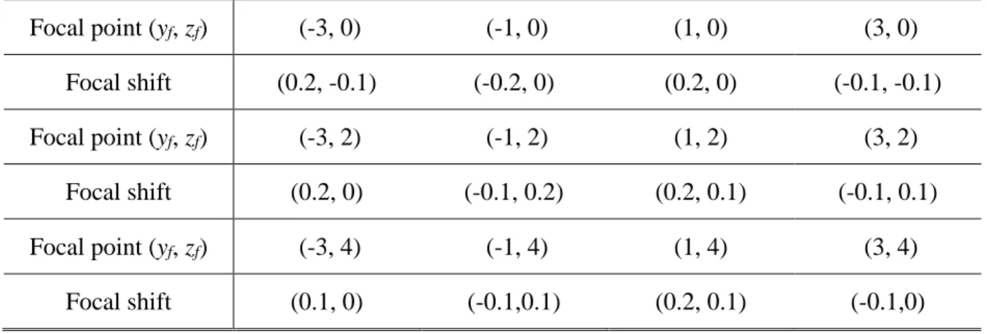
Table 4.1 Focal points and corresponding focal shift of matrix-form NFMF (unit: λ) ... 59
Table 4.2 Focal points and corresponding focal shift of circular form NFMF (unit: λ) ... 61
Table 4.3 Focal points and normalized amplitude of NFMF array prototype ... 88
Table 5.1 Cross-polarization on x = -8λ (Unit: dB) ... 105
LIST OF FIGURES
Figure 1.1 Proposed 5G network and key techniques in 5G networks [3] ... 2 Figure 1.2 NFF technique: (a) planar array for NFF with excitations subjecting to conjugate-phase approach; (b) power pattern in the near-field region realized by an 88 NFF array[7] ... 3 Figure 1.3 8×8 NFMF array (12 GHz) based on numerical algorithm and its corresponding
near-field pattern with a focal distance of 4.8λ (120mm) [14] ... 4 Figure 2.1 Near-field and far-field region of antenna. ... 8 Figure 2.2 Infinitesimal dipole equivalent models for different types of antennas (blue arrows represent infinitesimal electric dipoles, and red arrows represent infinitesimal magnetic dipoles): (a) half-wave dipole; (b) leaky-wave antenna; (c) patch antenna; (d) horn antenna. ... 11 Figure 2.3 Procedure for building an infinitesimal dipole equivalent model for near-field estimation. ... 13 Figure 2.4 Patch antenna and the corresponding infinitesimal dipole model: (a) configuration of infinitesimal dipoles; (b) position for near-field estimation; (c) far-field results on plane θ = 90º; (d) far-field results on plane ϕ = 180º; (e) near-field estimation (x = -8λ, z = 0) ... 13 Figure 2.5 Schematic of N-element near-field array focusing at point f with excitations obeying the conjugate-phase approach. ... 15 Figure 2.6 Near-field focusing cases: (a) focusing on standalone focal point f1; (b) focusing on standalone focal point f2; (c) focusing on focal point f1 and f2 simultaneously. ... 16 Figure 2.7 N-element linear antenna array focusing at focal point fm with: (a) even number of antennas; (b) odd number of antennas. ... 18 Figure 2.8 AF of antenna array: (a) case of focusing at single focal point; (b) case of focusing at multiple focal points with minimum distance. ... 20 Figure 2.9 N-element linear array: (a) θm = 0, relationship between focusing resolution R and lm; (b) focal plane x = -8λ, relationship between R and θm. ... 23
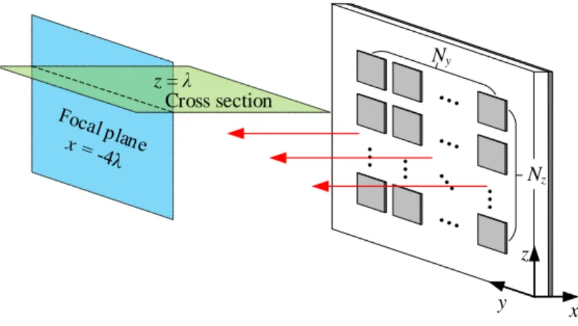
Figure 2.10 General procedure of the proposed NFMF method. ... 24 Figure 2.11 Configuration of antenna and array: (a) patch antenna element and the corresponding infinitesimal dipole equivalent model; (b) rectangular lattice array composed of patch antennas for NFMF. ... 25 Figure 2.12 Configuration of transmitting antenna array on yoz plane and focal plane on yz-plane.
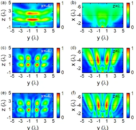
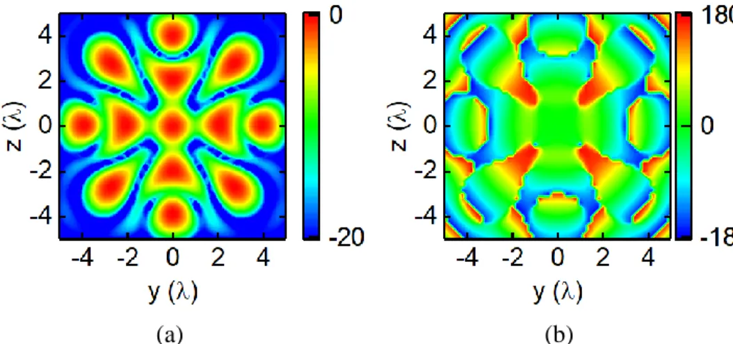
... 26 Figure 2.13 Normalized E-field distribution of NFMF on focal plane x = -4λ and cross section z =
λ, respectively: (a) & (b) Ny = 7 < Ny,min, Nz = 12; (c) & (d) Ny = 12 = Ny,min, Nz = 12; (e) & (f)
Ny = 16 > Ny,min, Nz = 12. ... 27 Figure 2.14 Normalized E-field distribution of NFMF on focal plane x = -4λ: (a) circularly distributed focal points; (b) linearly distributed focal points. ... 28 Figure 3.1 Block diagram of a typical genetic algorithm. ... 32 Figure 3.2 Procedure of element tuning-based algorithm for NFMF. ... 33 Figure 3.3 Normalized E-field distribution of NFMF on focal plane x = -8λ: (a) Ny = Nz = 10; (b)
Ny = Nz = 11; (c) Ny = Nz = 14. ... 35 Figure 3.4 Configuration of NFMF array for focal shift correction. ... 37 Figure 3.5 Focal shift correction of two focal points simultaneously: (a) normalized E-field for initial case on x=-4λ; (b) normalized field for optimized case on x=-4λ; (c) Normalized E-field distribution along transmitting direction of each focal points for both initial case and optimized case. ... 38 Figure 3.6 Pattern of amplitude (left) and phase (right) of NFMF array with in-phase and
equal-amplitude conditions: (a) initial case; (b) optimized case. ... 41 Figure 3.7 Configuration of back-fed patch antenna: (a) patch antenna fed by vertical located coaxial line; (b) patch antenna fed by microstrip line through coupling slot on the ground layer. ... 42 Figure 3.8 Configuration of Pi network as phase and amplitude tuning method. ... 43
Figure 3.9 Cascaded Pi networks for multiple outputs with unequal distributed amplitude and
phase. ... 44
Figure 3.10 Configuration of planar feeding networks for planar array with NaNb elements. ... 44
Figure 3.11 Configuration of unequal-split power divider. ... 45
Figure 3.12 Prototype of antenna array for NFMF: antenna layer, ground layer, and layer for feeding network. ... 47
Figure 3.13 Configuration of testing environment and signal flow. ... 48
Figure 3.14 Facilities and testing environment. ... 48
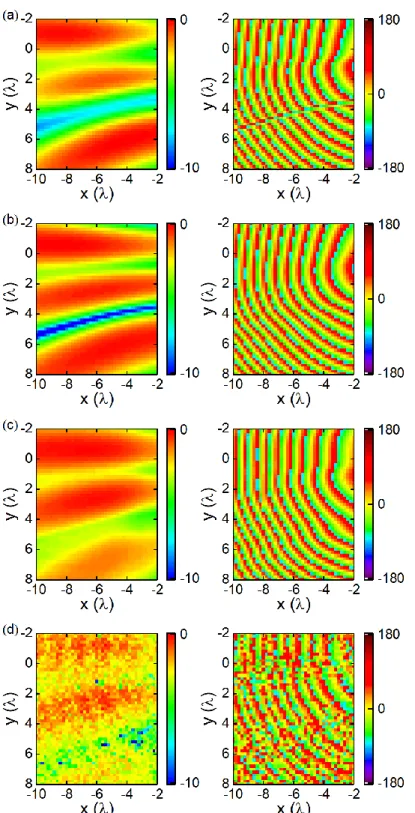
Figure 3.15 Amplitude and phase distribution on focal plane z = -8λ: (a) calculation without optimization; (b) calculation with GA optimization; (c) full-wave simulation based on optimized case; (d) experimental results based on optimized case. ... 49
Figure 4.1 Illustration of pattern-tuning based algorithm including three focal points with different amplitude. ... 54
Figure 4.2 Block diagram for pattern tuning-based NFMF array. ... 55
Figure 4.3 Configuration and procedure of the spatial signal processing. ... 57
Figure 4.4 Schematic of spatial power splitting with one input and spatially distributed multiple outputs with equal or unequal power ratio. ... 58
Figure 4.5 Example of spatial power splitting with matrix-form distributed targets: (a) normalized amplitude (dB); (b) phase (degree). ... 59
Figure 4.6 Example of spatial power splitting with circular distributed form distributed targets: (a) normalized amplitude (dB); (b) phase (degree). ... 60
Figure 4.7 Procedure of pattern shaping on continuous focal region. ... 62
Figure 4.8 Example of 1-D converging case with dual sub-regions. ... 63
Figure 4.9 Distribution of sampling spots for NFMF in a square region (dashed line). ... 64
Figure 4.10 Spatial power combining on square region with uniform distribution: (a) amplitude (dB); (b) phase (degree). ... 65
Figure 4.11 Field distribution of spatial power combining on square region along z = 0 on focal plane. ... 65 Figure 4.12 Distribution of sampling spots for NFMF in a circular region (dashed line). ... 66 Figure 4.13 Spatial power combining on circular region with uniform distribution: (a) amplitude (dB); (b) phase (degree). ... 67 Figure 4.14 Field distribution of spatial power combining on circular region along z = λ on focal plane. ... 67 Figure 4.15 Spatial power combining on square region with: (a) sinusoidal amplitude (dB); (b) uniform phase (degree) distribution. ... 68 Figure 4.16 Field distribution of spatial power combining on square region with sinusoidal amplitude along z = 0 on focal plane. ... 69 Figure 4.17 Spatial power combining: (a) schematic of spatial power combining with single source; (b) schematic of spatial power combining with multiple sources. ... 70 Figure 4.18 Schematic of multiple areas spatial phase shifting with identical or different phase delay in each region with specified shapes. ... 70 Figure 4.19 Distribution of sampling spots for NFMF in triple square regions (dashed line). ... 71 Figure 4.20 Spatial phase shifter: (a) example of spatial phase shifting on three square regions with uniform amplitude in each region; (b) corresponding phase delay of -90, 0, 90 degrees in each region. ... 72 Figure 4.21 Spatial phase shifting on single square region with: (a) uniform amplitude (dB); (b) linearly varied phase (degree) distribution. ... 73 Figure 4.22 Field distribution of spatial phase shifting on square region with linearly varied phase along z = 0 on focal plane... 73 Figure 4.23 Configuration of parallel feeding networks: (a) conventional SIW based parallel feeding network for equal power distribution; (b) end-loaded parallel feeding network for unequal power distribution. ... 75 Figure 4.24 Architecture of SIW-based phase-shifter-attenuator. ... 76
Figure 4.25 Configurations of conventional and proposed components: (a) conventional schematic of planar SIW hybrid coupler reflection type phase-shifter; (b) side view of the proposed folded SIW structure and its equivalent circuit; (c) reflective load in the proposed design and
its equivalent circuit. ... 77
Figure 4.26 Frequency response of proposed device by tuning wi (ls = 46 mils): (a) S21 phase; (b) S21 amplitude. ... 78
Figure 4.27 Frequency response of proposed device by tuning ls (wi = 185 mils): (a) S21 phase; (b) S21 amplitude. ... 79
Figure 4.28 Top and bottom view of the prototypes of phase-shifter-attenuator circuit with microstrip to SIW transitions. ... 80
Figure 4.29 Results of prototypes with different wi (ls = 0 mil): (a) measured and simulated results of S21 phase; (b) measured and simulated results of S21 amplitude. ... 81
Figure 4.30 Configuration of feeding networks: (a) end-loaded parallel feeding network; (b) distributed parallel feeding networks. ... 82
Figure 4.31 SIW T-junction featuring a function of power and phase allocation. ... 83
Figure 4.32 Simulation results of amplitude and phase tuning of SIW T-junction with different l1 and l2: (a) amplitude ratio (dB) between output ports 2 and 3; (b) phase difference (degree) between output ports 2 and 3; (c) S11 (dB) of T-junction. ... 84
Figure 4.33 Configuration of millimeter-wave NFMF array and corresponding feeding networks. ... 85
Figure 4.34 Prototype of 4×4 NFMF array: (a) antenna array as top layer; (b) corresponding distributed feeding network as bottom layer. ... 86
Figure 4.35 Schematic of testing environment. ... 86
Figure 4.36 Practical testing environment for near-field scanning of 4×4 NFMF array. ... 87
Figure 4.38 Near-field pattern of prototype: (a) simulated performance of prototype involving nine discrete converging targets on plane x = -8 with a matrix form distribution; (b) measured performance of prototype. ... 88 Figure 5.1 Near-field AF calculated at a distance of 8 away from linear array of 10 antenna elements with conjugate-phase and different amplitude weights w including: uniform weight (green line); Dolph-Chebyshev weight with 20 dB SLL (blue line); Dolph-Chebyshev weight with 40 dB SLL (red line); binomial weight (black line). ... 94 Figure 5.2 Two types of architectures of dual-polarization near-field antenna array: (a) hybrid array with separated vertically and horizontally polarized sub-arrays; (b) hybrid array with interwoven-style vertically and horizontally polarized sub-arrays. ... 96 Figure 5.3 Proposed T-junction for amplitude and phase allocation: (a) original design of feeding networks tuned by two parameters along horizontal direction; (b) schematic of improved T-junction including three geometric parameters l1, l2 and l3 introduced for tuning purpose. .. 97 Figure 5.4 Equivalent model of the proposed T-junction. ... 97 Figure 5.5 Amplitude and phase tuning results of the T-junction with different l1, l2 and l3. ... 98 Figure 5.6 Block diagram for design NFMF array with polarization diversity. ... 100 Figure 5.7 NFMF on multiple targets with orthogonal polarizations at plane x = -8λ: (a) E-field components along horizontal direction; (b) E-field components along vertical direction. .. 102 Figure 5.8 Normalized E-fields of NFMF on triple square regions with horizontal, vertical and 45 polarization respectively at x = -8λ: (a) field component along horizontal direction; (b) field component along vertical direction; (c) field component along 45 direction; (d) E-field components along 135 direction... 102 Figure 5.9 NFMF array focuses on two square areas having orthogonal polarizations with different amplitude weights: (a) uniform; (b) Chebyshev with -20 dB SLL; (c) DolphChebyshev with 40 dB SLL; (d) binomial; (e) hybrid (uniform and DolphDolphChebyshev with -40 dB SLL). ... 104 Figure 5.10 44 interwoven array and the corresponding SIW feeding networks. ... 106
Figure 5.11 Prototype of 4×4 NFMF array: (a) top layer for dual-polarization array; (b) bottom layer for improved distributed feeding network. ... 107 Figure 5.12 Schematic of dual-polarization test of NFMF array. ... 107 Figure 5.13 Configuration of the testing platform and the installation of NFMF array. ... 108 Figure 5.14 NFMF on two discrete focal points with 45 and 135 polarization respectively: (a) Calculation results of E-field components along different directions; (b) Simulation results of E-field components along different directions; (c) Experimental results of E-field components along different directions. ... 109
LIST OF SYMBOLS AND ABBREVIATIONS
4G The fourth generation of broadband cellular network technology 5G The fifth generation cellular network technologyAF Array factor
GA Genetic algorithm
LM Levenberg-Marquardt algorithm MIMO Multiple-input and multiple-output
NF Near field
NFF Near-field focus NFMF Near-field multi-focus PSO Particle swarm optimization
RF Radio frequency
SIW Substrate integrated waveguide SLL Side-lobe level
CHAPTER 1
INTRODUCTION
1.1 Background
For the fifth generation (5G) wireless communication system, the network is supposed to provide up to ten gigabit-per-second average data transmission rates in support of high-speed datalink, autonomous driving and other applications. As a result, networks and devices should be developed to feature high spectrum efficiency, high energy efficiency, high power capacity and low connection latency, which are essential in fulfilling the ultra-high-speed requirement of 5G networks.
As a key technique in the 4G wireless network, the multiple-input multiple-output (MIMO) scheme has been widely used as it offers multipath transmitting and receiving functions, which ensure its high spectral efficiency [1]. In the 5G wireless system, the concept of MIMO is again continued to be applied by adding multiple antennas in both transmitters and receivers on a much larger scale compared to its 4G counterpart, usually tens or even hundreds of antennas. In this case, the spectral efficiency could be enhanced in a significant manner, which is now named massive MIMO system. Small cells are introduced as base stations to ensure the capability of handling a high data rate of signal transmission, which commonly includes femtocells, picocells and microcells. They feature low power and high geometrical density to cover the communication in a small area compared with the conventional macro base station. A shorter or even line-of-sight distance between small cells leads to higher capacity of the network. In addition, a combined network of macro base stations and small cells is robust and flexible with high spectral efficiency for a complex environment [2]. In the 5G network, another key problem is energy efficiency, as the fading scenario in an environment would influence the quality of communications a lot. With the help of massive MIMO and small cells, indoor scenarios (line-of-sight or pure environment) are connected to outdoor scenarios (noisy environment with multipath interference) with lower penetration loss. By doing so, the spectral and energy resources can be allocated separately in different scenarios in order to save energy. In view of circuit and source types, millimeter-wave and visible light communication techniques would be considered as suitable solutions.
In all 5G and future wireless communication systems, high spectrum efficiency and high energy efficiency are expected to be two important metrics that are usually used to highlight the requirements related to the scenarios of high data rate and multiple user terminals (Figure 1.1).
Figure 1.1 Proposed 5G network and key techniques in 5G networks [3]
As a result, proximity or short-range wireless devices and systems have become flourishing thanks to their potential integration with various handheld mobile and flexible or wearable platforms. Therefore, simultaneous wireless power, data transmission and sensing operation within a near-field region may become an indispensable or even a desired choice in support of emerging super-high-speed wireless applications such as 5G and beyond. Depending on the target range and operating wavelength, more signal routing and lower transmission loss can readily be achieved in the Fresnel region (radiative near-field region) compared to the far-field region. In order to increase the power/energy efficiency further and/or to deploy low-loss spatial powering or signal delivery, flexible near-field focusing (NFF) and multi-focus beaming techniques are preferred and should be created.
Similar to the operation of a convex lens used over the visible light band, the power transmission or signal delivery of an antenna array can be concentrated at a focal point or distributed in the area around that point. This can be enabled by the use of an NFF technique. In the NFF technique, a conjugate-phase approach is utilized to designate the phase of an excitation signal for each element in the transmitting array such that the transmitted wave of each antenna is in phase at the focal point [4-6]. Research work related to NFF has been conducted since the last century including the
development of the principles and features of NFF [7-11], the schematic of NFF array based on the conjugate-phase approach and corresponding near-field pattern is displayed in Figure 1.2. The optimization and shaping/synthesis of fields in NFF scenarios have been also considered [12, 13].
(a) (b)
Figure 1.2 NFF technique: (a) planar array for NFF with excitations subjecting to conjugate-phase approach; (b) power pattern in the near-field region realized by an 88 NFF array[7]
NFF is known to offer a solution for efficient power transfer, communication and imaging in a short range. Moreover, a near-field technique is now evolving to what should support multiple targets at random locations and/or serves as a wireless power transfer of multiple devices. By assigning an appropriate condition of excitation related to amplitude and phase for each antenna in an array, the resulting antenna array is able to exhibit multiple focal points in a near-field region. This phenomenon is called near-field multi-focus (NFMF), which may provide an alternative approach to the classical power/signal combining and splitting through physically-connected transmission lines. It also offers a solution for the communications of small cells in the case of multi-users. By applying this technique, power/signals from transmitters are concentrated at multiple focal points or areas instead of radiating to the entire space.
Figure 1.3 8×8 NFMF array (12 GHz) based on numerical algorithm and its corresponding near-field pattern with a focal distance of 4.8λ (120mm) [14]
Earlier works have been carried out about NFMF concerning the focusing algorithm, optimization method, field model, RF front-end and related circuits. Ayestarán et al. realized the focusing of two points with a planar antenna array [14-17], whose prototype and corresponding near-field pattern are shown in Figure 1.3. Feeding weights for amplitude and phase were introduced to define the excitation condition of each antenna. Levenberg-Marquardt algorithm was used for optimizing the values of those weights in order to achieve the desired focusing status. Furthermore, the mutual coupling between antennas was taken into account with neural networks [18, 19]. By employing a coupling matrix in the weight evaluating process, the accuracy of the model and values of excitation can be enhanced. Cheng et al. concentrated on designing the RF front-end design of NFMF, and their leaky-wave antenna is able to accomplish the sweeping beam in the near-field region with continuously varied operating frequency [20]. Not only the antenna array but also the lens placed before the antennas can change the focusing status. Hassan et al. developed a porous dielectric lens for changing the phase condition in the near-field region [21], a symmetrical beam with angle of 40 degrees in both near-field and far-field was successfully proposed and realized.
Previous research work was mainly focusing on defining the spatial locations of multi-focus points, while some key features of multi-focus were merely mentioned such as focal width, focal shift, focusing resolution, polarization, amplitude and phase distribution, and so on. In addition, the algorithms for NFMF are numerical-solution-based, whose computational speed mainly relies on the convergence speed of the optimization method adopted. As a result, the previous solutions are
suitable for NFMF with fixed locations. Functions such as multiple beam tilting and multi-target tracing are hardly realized because the numerical solution is not fast enough.
1.2 Research objectives and methodologies
With the above-mentioned background work in mind, a method for NFMF is proposed and demonstrated in this research work. The method of designing a multi-focus antenna array is developed and improved in different aspects. It is detailed and validated in the thesis through both theoretical and experimental approaches.
The first goal is the development of an analytical algorithm for NFMF. The computational speed of the numerical algorithm adopted in the previous works is mainly constrained by the convergence rate of iteration in the optimization method, which is not suitable for circumstances with multiple movable focal targets or with a large number of focal points. In this work, an analytical algorithm will be developed, which features high computational efficiency.
The second goal is the expansion of focusing abilities. In conventional works, NFMF is only valid at several discrete points in the Fresnel region. While in this work, a large number of focal points can be defined by the proposed method. Moreover, a focusing phenomenon on multiple continuous regions with regular or irregular shapes is exploited and investigated, which performs as a pattern shaping in the near-field region.
The third goal is the understanding and exploitation of unique geometrical features in NFMF. Different from NFF patterns, an NFMF pattern has some unique geometrical features due to the coexistence of multiple focal points. For example, the focusing resolution is defined in NFMF to clarify the minimum spacing between two adjacent focuses that are distinguishable from each other. The relationship between the scale of a near-field antenna array and its corresponding resolution is investigated in this work. Interesting technical features such as focal depth and focal width of NFMF are explored too.
The last goal of this work is related to some concrete applications of NFMF. As NFMF is able to perform pattern shaping, the applications can be expected in many ways such as power combining or splitting, energy delivery and allocation, signal processing, and polarization diversity. These
applications are accomplished in a spatial way, and they are promising for a wide range of system and device applications such as 5G networks.
The framework of this research description through this thesis is arranged as follows.
In Chapter 2, the fundamental theories for developing NFMF antenna arrays are introduced and investigated. Near-field antenna and corresponding field model are studied for analytical estimation of field behavior of the proposed NFMF arrays. Subsequently, the conjugate-phase approach is formulated and improved with a superposition theorem, which serves as the foundation for the proposed analytical algorithm. Furthermore, the concept of near-field array factor is introduced, and then the focusing resolution is developed with the help of a near-field array factor to estimate the proper array scale for a specified NFMF condition. Finally, the procedure of designing an NFMF antenna array is developed and discussed.
In Chapter 3, the NFMF method is further developed by introducing the tuning factor for each antenna element. By introducing the element-based tuning factors, not only locations, but also amplitude and phase of each focal point can be specified with a semi-analytical algorithm with the help of iterative optimization method. With this improved method, the field distribution can be specified on or around the focal points. Array and corresponding microstrip-line based circuits are designed and tested in X-band for demonstration purposes.
In Chapter 4, the function of NFMF arrays is further extended by introducing a pattern based tuning vector. Different from the element-based tuning, pattern-based tuning can be achieved without adopting any optimization method. As a result, the pattern-based tuning algorithm can deal with NFMF having a large number of focal points with a rapid computational speed. With this algorithm, the antenna array is able to focus on not only discrete points, but also continuous regions with specified shapes as an ability of near-field pattern shaping. This feature provides a foundation for accomplishing many circuit and system functions such as power combing, power splitting and signal processing in the near-field region, which is discussed and demonstrated theoretically and experimentally in this thesis.
In Chapter 5, the NFMF method is improved with a function of polarization diversity. In the conventional NFMF method, the antenna array is identically polarized and all the focal points share the same polarization. In this chapter, an algorithm for polarization allocation on multiple focal
points or regions is formulated. Furthermore, cross-polarization isolation of each focal point or region can be controlled by the proposed method. Corresponding dual-polarized array and SIW based circuit are designed and fabricated for demonstration purpose in millimeter-wave band. In Chapter 6, the research work is concluded, current issues and future work are discussed to appreciate the tremendous values and potential impacts of this research.
CHAPTER 2
THEORY OF NEAR-FIELD ARRAY FOR MULTI-FOCUS
The behavior of antenna arrays is generally determined by their antenna elements. To develop the multi-focus antenna arrays in the near-field region, the properties of an antenna near-field and corresponding model are introduced in this chapter. Furthermore, an analytical algorithm is developed for NFMF, and the procedure of designing an NFMF array is discussed.2.1 Antenna near field
2.1.1 Near field
Antenna near-field (reactive and Fresnel) region and far-field (Fraunhofer) region are the regions around antenna which are defined by distance. For an antenna or array physically larger than a half-wavelength with maximum geometrical length D, its far-field region is defined with distance
2
2
r D , and the reactive region is located in a range of
3
1 20.62
r D , while the Fresnel region is defined as the space between them [22] (Figure 2.1).
Reactive region Fresnel region Fraunhofer region Near-field Far-field 2 2D 3 0.62 D
Figure 2.1 Near-field and far-field region of antenna.
In conventional research, performances like pattern and polarization are investigated in connection with the far-field regions as antennas are mainly applied as part of transmitters or receivers with a relatively long distance from the originating radiation source. However, the field property in the near-field region is different from that in the far-field region.
First of all, we need to highlight that when an antenna is utilized within the near-field region, the nature of electromagnetic waves it transmits is different from that in the far-field region. With the
help of a Wilcox expansion [23], the space-expanding electromagnetic waves generated from a source of radiation can generally be expressed by [24]
0 0 , , jkr i i i jkr i i i e r r e r r
A E r B H r . (2.1)The above equations cover the entire space around an antenna in question including near-field and far-field regions. It can be observed that in the near-field region the electromagnetic field is formulated as a function of the combination of 1/ri (i = 1,…∞). While in the far-field region, high-order terms of 1/r can be neglected with increasing r, which can be simplified as
0 0 , , jkr jkr e r e r A E r B H r . (2.2)The above-described equation is coincident with the classical expression of antenna fields for the far-field region. The difference in expression between the near-field and far-field regions is caused by the different types of energy that these two regions accommodate. In the far-field region, only radiative energy takes place. However, in the near-field region, there exist both radiative energy and reactive energy simultaneously. The higher-order terms of 1/r stand for the reactive energy that is maintained or transmitted inside the near-field region. As the distance goes far and far away from the antenna, the reactive energy becomes weaker and weaker. Therefore, only radiative energy exists in the far-field region. However, to estimate or evaluate the field behavior in the near-field region, both reactive and radiative energy should be taken into consideration.
On the other hand, the transmission mode in the near-field region is different from that in the far-field region. In the far-far-field region, the electromagnetic wave radiates with a TEM mode as there are no longitudinal electric and magnetic components (in the propagation direction) with a boundary condition of free space. However, in the near-field region, the modal behavior is quite astonishing because of reactive energy. By solving the Wilcox expression with spherical harmonics, the electromagnetic waves can be expressed with both TEr and TMr modes in the near-field region as follows [24]:
1 1 lm 1 1 lm , , TE mode 0 , , TM mode 0 l l TE lm E k l lm TE lm l l TE lm M k l lm TE lm a l m h kr Y a l m h kr Y r H r E r E r H . (2.3)The equations (2.3) define the transmission modes in the near-field region with spherical Hankel functions. Waves in the near-field region are transmitted with TEr, TMr modes or a combination of them as the longitudinal field component exists due to the reactive field in this region [24, 25]. In the end, the behavior of electromagnetic waves in the near-field region is different from those in the far-field region. Therefore, the behavior of electromagnetic fields in the near-field region cannot be evaluated by the conventional approach deployed for the far-field region.
2.1.2 Near-field models
Specific models or methods need to be introduced for the field evaluation related to the near-field region. As a classical approach, the dyadic Green function theorem makes use of the current distribution of antenna to calculate the E-field in the near-field region [26, 27]. Another approach is the use of a far-field-to-near-field (FF-NF) transformation method [24], combining the Wilcox expansion with antenna radiation pattern in the far-field, E-field in the near-field region can then be derived. With reference to each other, the dyadic Green function theorem is used to derive the fields from the source while the FF-NF transformation method relies on the far-field. Both of them require a massive data acquisition to ensure the accuracy of the finally derived fields.
In the previous works, the concept of equivalent source model was adopted in predicting and estimating of the field behavior, which accomplished near-field-to-far-field transformation [28, 29], also some applications in the area of antenna measurement [30, 31]. In order to accelerate the field calculation process while maintaining an excellent accuracy, an infinitesimal dipole equivalent model [32, 33] is studied and adopted as the antenna near-field model in this work. The main idea of this equivalent method is to synthesize a specific radiation pattern of a single antenna with a cluster of infinitesimal dipoles. It combines the background thoughts of the dyadic Green function and the FF-NF transformation method altogether. With regard to the aspect of a current source, an infinitesimal dipole antenna has a simple current distribution, by which a quasi-analytical
closed-form expression of field distribution in both near- and far-field regions can be provided in a concise manner. With regards to radiation pattern, an arbitrary form of antenna can be equivalently thought of as a group of infinitesimal electric or magnetic dipoles or their combinations. Previous researches point out that, the entire field in the exterior region of an antenna can be completely determined from the radiation pattern [23], and a given far-field radiation pattern of antenna can be used to estimate its near-field field distribution except the field close to the source with evanescent modes [24, 27].
(a) (b)
(c)
(d)
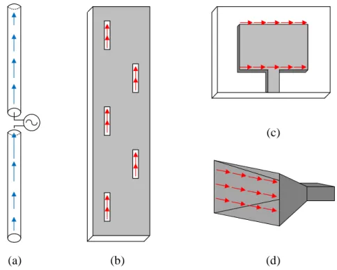
Figure 2.2 Infinitesimal dipole equivalent models for different types of antennas (blue arrows represent infinitesimal electric dipoles, and red arrows represent infinitesimal magnetic dipoles): (a) half-wave dipole; (b) leaky-wave antenna; (c) patch antenna; (d) horn antenna.
For a conventional antenna with a regular shape, the basic forms of an equivalent model based on electric or magnetic infinitesimal dipoles can be predefined. Figure 2.2 shows some models for typical antennas. Dipoles such as half-wave dipole and broadband dipoles or monopoles can be treated as a cluster of infinitesimal electric dipoles, while the slot antenna, horn antenna, leaky-wave antenna and patch antenna can be represented by infinitesimal magnetic dipole as their apertures are mainly slots.
Following the creation of an initial equivalent model, parameters of infinitesimal dipoles such as location, and excitation status and so on require optimization to fit with the radiation pattern of a target antenna. With the optimized parameters, the E-field pattern of an antenna can be written as
1 1 Q P p q p q A A
E p
M q E r E r E r , (2.4)where P and Q are the total numbers of infinitesimal electric and magnetic dipoles defined in the equivalent model, respectively. The number and location of the infinitesimal dipoles are determined by the antenna type and its current distribution. In addition, the parameters such as location, amplitude and phase of infinitesimal dipoles adopted are to be optimized to get an accurate model of the selected antenna. rp and rq stand for the vectors pointing form infinitesimal dipoles
to target point. EE (EM) represents the general E-field of the infinitesimal electric (magnetic)
dipoles that are valid for either estimated near-field or synthesized far-field as
2 3 2 0 2 1 3 4 1 1 4 jkr jkr o e k jk r r r e k Z r jkr E M E n p n n n p p E n m , (2.5)where n is the unit vector pointing to target point; p and m are the electric and magnetic dipole moment, respectively; Z0 stands for the impedance of free space, and k is the wavenumber. The detailed procedure of building such an infinitesimal dipole model is shown in Figure 2.3. Let’s consider the patch antenna in Figure 2.4(a) as an example. The antenna is located at the center of Cartesian coordinate with its broadside pointing to negative x-direction. This antenna is represented by a 5×2 array of infinitesimal magnetic dipoles which are located at the edges perpendicular to the polarization direction. As mentioned above, the near-field pattern can be estimated by a given far-field pattern. As a result, we can optimize the location, the amplitude and phase of the infinitesimal dipoles to fit with the far-field result of the target antenna obtained by full-wave simulations or experimental tests in order to generate the near-field model of the chosen antenna element.
No Calculate far-field
Coincident with full wave results?
Yes Build model & parameters
Calculate near-field
Figure 2.3 Procedure for building an infinitesimal dipole equivalent model for near-field estimation. y x z NF estimation position x = -8λ z = 0 Antenna x y o (a) (b)
Figure 2.4 Patch antenna and the corresponding infinitesimal dipole model: (a) configuration of infinitesimal dipoles; (b) position for near-field estimation; (c) far-field results on plane θ = 90º; (d) far-field results on plane ϕ = 180º; (e) near-field estimation (x = -8λ, z = 0)
Figure 2.4 (c) and (d) show the full-wave simulation-based far-field of the antenna and the fitting results of its equivalent model. With the optimized equivalent model, the near-field distribution on
estimation position (Figure 2.4(b)) of the equivalent model is calculated and compared with the full-wave simulation-based near-field of the antenna element in Figure 2.4(e), which shows an agreement between each other with a minor difference.
As mentioned above, the equivalent model adopted for the patch antenna is composed of two group of infinitesimal magnetic dipoles, which represent the ideal case of the patch antenna. While the practical patch would introduce cross-polarization and other radiation caused by finite ground, which leads to the difference between simulated and calculation results. The accuracy of this model can be further improved when introducing more infinitesimal dipoles in the equivalent model [34]. With the near-field equivalent model, we can now calculate fields at certain locations through the quasi-analytical equation discussed above instead of time-consuming full-wave simulations.
2.2 Near-field multi-focus
The physical focusing of transmitted energy by a cluster of antennas is a field interference phenomenon in nature. Physically alternating constructive or destructive interferences can define specific areas with increased or decreased wave/field strength. Furthermore, the antenna array with designated amplitude and phase conditions can form a specified or wanted interference pattern at certain locations in an open space. In order to converge the maximum power at one specified point in the near-field region, a conjugate-phase approach was utilized to designate the phase of an excitation signal for each element in the array [4-6].
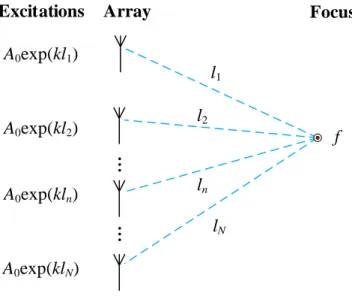
In the conjugate-phase approach, the antenna array is composed of N identical elements (Figure 2.5). All the elements are excited with identical amplitude, while the phases of excitations are different for the convergence purpose, which obeys the rule of “conjugate-phase”. Electromagnetic wave transmitted from nth antenna to a certain focal point has a phase delay of -kln, where k is the wavenumber and ln is the geometrical distance from the nth antenna to the focal point. To make sure that waves from all the elements are converged at the specified focal point with the maximum power level, the waves should be superimposed with an in-phase condition. The in-phase condition can be artificially created by applying conjugate-phase n = kln (n = 1, 2… N) as the phase of excitation. This conjugate-phase compensates the phase difference at the focal point introduced by different positions of antennas, so it serves as the principal design technique for an NFF antenna array having single focal point.
However, in some application cases like multi-target communication and wireless power supply, a designed NFF array may be required to yield two or more focal points for which the conjugate-phase approach is no longer applicable because it is only capable of accounting for one focal point.
f A0exp(kl1)
A0exp(kl2)
A0exp(kln)
A0exp(klN)
Excitations Array Focus
l1
l2
ln lN
Figure 2.5 Schematic of N-element near-field array focusing at point f with excitations obeying the conjugate-phase approach.
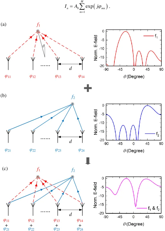
To realize a multi-focusing function of an antenna array, one should extend the conjugate-phase approach. For instance, the antenna array in Figure 2.6 is constructed to focus at f1 and f2 simultaneously. When the conjugate-phase approach is used for each standalone case, the proposed array is able to focus on single point as shown in (a) or (b). We can notice if the two focal points are located at the side-lobe region of each other. According to the superposition theorem, we can superimpose the two groups of excitation
11 14
0 , , 0 A e A e and
21 24
0 , , 0 A e A e , this combined excitation
11 21
14 24
0 , , 0A e e A e e is capable of generating two patterns with a superimposed status and yield the dual-focusing results simultaneously in (c).
The proposed method is also applicable to the case of multiple focal points. For N elements array with M focal points, the phase compensation for element n corresponding to focus m is
2
2
2mn k xm xn ym yn zm zn
By calculating (2.6), M groups of excitations are obtained for the antenna array. Taking the normalized amplitude into account, the excitation signal for each antenna is defined by
0 1 exp M n mn m I A j
. (2.7) f2 f1 d f2 d f1 d φ11 φ12 φ13 φ14 φ21 φ22 φ23 φ24 φ11 φ12 φ13 φ14 φ21 φ22 φ23 φ24 + + + + (c) (b) (a) θFigure 2.6 Near-field focusing cases: (a) focusing on standalone focal point f1; (b) focusing on standalone focal point f2; (c) focusing on focal point f1 and f2 simultaneously.
With the above excitations, the field distribution in a near-field region can be written as
1 N n n I
n E r E r , (2.8)wherern
xx yn, y zn, zn
. We can see that E-field is calculated for the near-field region where the nature of electromagnetic waves is different from that in the far-field region. The E-field of each antenna can be expressed with the quasi-analytical infinitesimal dipole model as discussed earlier. As a result, the total E-field pattern for NFMF can be written as
1 1 1 Q N P p q n n p q I A A
E p
M q E r E r E r . (2.9)With this equation, the near-field distribution of the antenna array can be formulated for multiple focal points at the target location. The proposed method can realize a multi-focusing feature with designated excitation In (n = 1, 2… N) based on the improved conjugate-phase approach presented above. The infinitesimal dipole equivalent model is adopted for a quasi-analytical near-field expression. As the quasi-analytical expression of an infinitesimal dipole field is known, the estimation of the array’s near-field is fast, and the accuracy of the near-field pattern is determined by its equivalent model.
2.3 Focusing properties
The proposed method above offers an analytical derivation of excitations and an estimation of near-field, which targets two or more multi-focus points in the near-field region. While the properties of multi-focusing features rely not only on the excitations but also on the configuration of antenna array itself, such as the width of focal point, resolution, side lobe level etc. which are directly influenced by the array form. Therefore, the relationship between the configuration of the antenna array and the focusing properties will be discussed in this section.
In conventional research works, the antenna is located in a 2D plane with rectangular lattice [4-6, 35-38] as it is convenient to design, calculate and manufacture, and some properties of NFF are investigated and discussed [10, 11]. To simplify the calculation process, antenna elements in the
NFMF antenna array discussed in this work are equally spaced with a linear or rectangular lattice form. With this topology, some typical features will be discussed below.
2.3.1 Near-field array factor
Array factor (AF) is a common tool widely used in estimating the behavior or function of an array utilized in the far-field region as it can represent the general properties of an array with certain configuration and excitation condition. Furthermore, AF serves as an outline in designing the process of a far-field array. As the basic assumption of employing the AF, the array element is omnidirectional and the fields emitted by the array obey the superposition principle. Electromagnetic waves in the Fresnel region share the same properties in superpositionas those in the Fraunhofer region even though the energy in the Fresnel region is composed of both radiative and reactive ones. Therefore, in the Fresnel region, the concept of AF is also valid as an index for generally estimating the transmitting features such as main lobe direction, side-lobe level (SLL), beamwidth etc. regardless of the type of element in the near-field array.
In this section, we employ a “near-field AF” as a guiding parameter for designing an NFMF array governed by the proposed method.
fm d θm lm o fm o 1 2 -2 -1 -2 -1 0 1 2 d (a) (b) θm lm
Figure 2.7 N-element linear antenna array focusing at focal point fm with: (a) even number of antennas; (b) odd number of antennas.
To study the AF of an NFMF array, a linear N-elements array with equal spacing d serves as a typical example here. First of all, let us consider the case of mth focal point with a position of (lm,
θm) as described in Figure 2.7. Using the conjugate-phase approach, the excitation phase of element n is
2 2 2 2 2 sin 2 1 2 1 sin 2 omn m m m emn m m m k l nd nl d N odd n k l d n l d N even . (2.10)Assuming each element in the array shares the same normalized amplitude, i.e. A0=1, we can obtain the AF for the proposed array with the superimposed fields
2 2 2 2 1 2 2 sin 1 2 2 1 2 2 1 sin 2 2 1 m m omn m m emn N jk l nd nl d j N m n N jk l d n l d j N e N odd AF e N even
. (2.11)By employing the Taylor series of first order 1 x 1 x 2 with the condition of lm > Nd (which results in a maximum error of 2% in calculating the AF), where most of the radiative near-field region is considered, and the AF can be simplified as
sin 2 sin 2 m m m N AF , (2.12)
where m kd
sin sinm
. According to the superposition theorem, the general AF for a multi-focusing case 1 sin 2 sin 2 m M m m N AF
. (2.13)It is worthwhile to mention that approximations and assumptions are applied during the derivation of AF in (2.12) and (2.13) with a Taylor expansion in order to obtain a general analytical solution with concise expressions. The reason is that the above near-field AF serves as an approximate reference for deriving the required minimum scale of an antenna array for corresponding
multi-focus conditions in the following part. Therefore, one should refer to the accurate expression (2.9) in evaluating the exact near-field pattern or field distribution instead of considering the near-field AF.
It can also be noticed that the near-field AF derived above has a similar form as the conventional AF applied in the far-field region. However, they are different physically. The far-field AF is defined to calculate the only focal direction while the near-field AF is defined to estimate the focal point including both direction and distance simultaneously. Furthermore, the usage of them is also different. The AF for the far-field is used for calculating a far-field pattern of antenna array while the near-field AF derived above is adopted for estimating the scale of near-field antenna array. As a result, the near-field AF is specified for a near-field focus and cannot be applied to a far-field array even though they share a similar form.
2.3.2 Focusing resolution
With the above-described general near-field AF, we can investigate and estimate the properties of antenna array such as the geometrical parameters of antenna array for NFMF.
θm
Θ h
θm,-1 θm,1
θ θm-1θm θ
(a) (b)
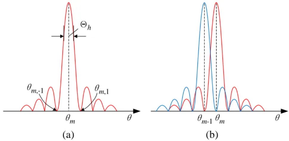
Figure 2.8 AF of antenna array: (a) case of focusing at single focal point; (b) case of focusing at multiple focal points with minimum distance.
For an antenna array with a high transmitting efficiency, the side-lobe or grating lobes should be prevented by adjusting the geometrical parameters of antenna array (Figure 2.8). Considering the case of a single focal point by solving (2.12), we can derive the peak(s) occurring at the direction
2 arcsin u sin m u kd . (2.14)We impose the AF to have only one peak that occurs at θm in the region
2, 2
to prevent the grating lobes. Under the circumstance of u = 0, and each nonzero u that cannot yield valid θ, we can then derive the range of distance between elements in an array by (2.14) as follows,max 1 sin m 2 d . (2.15)
Subsequently, we can come to the conclusion that in order to acquire NFF or NFMF in the half-space, the maximum distance dmax between neighboring antennas of an array should not be larger than a half free-space wavelength at operating frequency. Meanwhile, the spacing between elements also influences the mutual coupling effect between antennas. In order to reduce the coupling, antennas should be placed far away from each other. Therefore, a distance of half wavelength is mainly adopted as the spacing between antennas in this work.
The near-field AF derived above represents a general focusing property for multi-focus cases. Therefore, the concentrating level around each focal point in the case of NFMF can also be manifested. In the cases of a multi-focus development, depth of focus [7] is defined as the range between locations with -3-dB suppression around focal point along the broadside direction of antenna array; while focal width [7] is the corresponding -3-dB range along the direction parallel to antenna array. According to the expression of the derived near-field AF, it can estimate the trend of focal width at a focal plane for the multi-focus. By solving (2.12), we can derive Θh as the parameter representing the size of focal spot in one dimension of a general array with certain numbers of elements. As a result, the focal width of near-field array is positively correlated with Θh
2.782
focalwidth h arcsin sin m
kNd
. (2.16)This means that the focal width can be controlled by the number of antennas in each row or column in an array with fixed element spacing d. This suggests that a larger array scale should lead to narrower focal width and more concentrated transmitting energy.
As the NFMF feature is obtained by superimposing multiple near-field patterns, one cannot distinguish the two focal points if they are too close to each other. From (2.12), we know that the first zero-crossing response occurs at
, 1 2 arcsin sin m m kNd . (2.17)
In order to minimize the interference between the focal points, the focal point should be located at least away from the first zero-crossing region (Figure 2.8). Thus, we can obtain the minimum spacing between the focal points, i.e. the focusing resolution over the focal plane is
1 2
max mcos mtan sin sin m msin m
R l l kNd . (2.18)
The resolution defined above represents that of a one-dimensional condition, and the minimum spacing is defined as a line segment parallel to the linear array. For a two-dimensional case, the resolution should be calculated in two orthogonal directions according to the arrangement of antenna array. There are four main parameters that influence the focusing resolution R, including
lm, θm, N and d. In order to prevent grating lobes as discussed in the last part, d is fixed as a constant. In Figure 2.9(a), θm is fixed to be at 0 degree, and the focusing resolution of array with a different number of antennas is displayed. We can draw the conclusion that when more antennas are included in the array, the minimum spacing decreases, i.e. the focusing resolution can be improved by increasing the scale of array. Moreover, the focusing resolution could be better if the focal point is closer to the antenna array.
A similar conclusion can be drawn from Figure 2.9(b). In this figure, the focal plane is located at x = -8λ (array locates along yoz plane and faces negative x-direction) in order to detect the influence of θm. On one hand, the multi-focusing features are achieved in part of the space which is determined by the scale of antenna array N. For example, an array with four antennas can cover 96º, while an array with eight antennas can cover 120º, which is 25% wider than the former one. As a result, more antennas are employed and the NFMF will be realized in a wider space. On the other hand, with a fix scale N, the focusing resolution gets the best results when a focal point is located at θm = 0º, which is just facing the center of antenna array.