HAL Id: hal-02699213
https://hal.inrae.fr/hal-02699213
Submitted on 1 Jun 2020
HAL is a multi-disciplinary open access archive for the deposit and dissemination of sci-entific research documents, whether they are pub-lished or not. The documents may come from teaching and research institutions in France or abroad, or from public or private research centers.
L’archive ouverte pluridisciplinaire HAL, est destinée au dépôt et à la diffusion de documents scientifiques de niveau recherche, publiés ou non, émanant des établissements d’enseignement et de recherche français ou étrangers, des laboratoires publics ou privés.
with remotely sensed reflectance and surface
temperature : a case study for the HAPEX - Sahel
grassland sites
P. Cayrol, L. Kergoat, Sophie Moulin, Gérard Dedieu, A. Chehbouni
To cite this version:
P. Cayrol, L. Kergoat, Sophie Moulin, Gérard Dedieu, A. Chehbouni. Calibrating a coupled SVAT - vegetation growth model with remotely sensed reflectance and surface temperature : a case study for the HAPEX - Sahel grassland sites. Journal of Applied Meteorology, American Meteorological Society, 2000, 39 (12), pp.2452-2472. �10.1175/1520-0450(2000)0392.0.CO;2�. �hal-02699213�
q 2000 American Meteorological Society
Calibrating a Coupled SVAT–Vegetation Growth Model with Remotely Sensed
Reflectance and Surface Temperature—
A Case Study for the HAPEX-Sahel Grassland Sites
P. CAYROL
CNRS/CNES/UPS, Centre d’Etude Spatiale de la Biosphere, Toulouse, France
L. KERGOAT
CNRS/UPS, Laboratoire d’Ecologie Terrestre, Toulouse, France
S. MOULIN ANDG. DEDIEU
CNRS/CNES/UPS, Centre d’Etude Spatiale de la Biosphere, Toulouse, France
A. CHEHBOUNI
IRD/IMADES, Institut de Recherche pour le Developpement, Hermosillo, Mexico
(Manuscript received 30 August 1999, in final form 7 February 2000)
ABSTRACT
Models simulating the seasonal growth of vegetation have been recently coupled to soil–vegetation–atmosphere transfer schemes (SVATS). Such coupled vegetation–SVATS models (V–S) account for changes of the vegetation leaf area index (LAI) over time. One problem faced by V–S models is the high number of parameters that are required to simulate different sites or large areas. Therefore, efficient calibration procedures are needed. This study describes an attempt to calibrate a V–S model with satellite [Advanced Very High Resolution Radiometer (AVHRR)] data in the shortwave and longwave domains. A V–S model is described using ground data collected over three semiarid grassland sites during the Hydrological Atmospheric Pilot Experiment (HAPEX)-Sahel experiment. The effect of calibrating model parameters with time series of normalized difference vegetation index (NDVI) and thermal infrared (TIR) data is assessed by examining the simulated latent heat flux (LE) and LAI for a suite of calibration experiments. A sensitivity analysis showed that the parameters related to plant growth vigor and to soil evaporative resistance were the best candidates for calibration. The NDVI and TIR time series were used to calibrate these parameters, both independently and simultaneously, to assess their synergy. Ground-based, airborne, and satellite sensor (AVHRR) data were successively investigated. Both air-borne and AVHRR NDVI data could be used to constrain the vegetation growth vigor. These calibrations significantly improved the simulation of the LAI and LE (rmse decreased by 21% for LE), and the site-to-site variability was greatly enhanced. The soil resistance could also be calibrated with ground-based TIR data, but the effect on the simulated variables was small. Although both NDVI and ground-based TIR data were suitable to constrain the V–S model, the synergy between the two wavelengths was not clearly established. Last, satellite TIR data from the AVHRR proved unsuitable for model calibration. Indeed, the AVHRR surface temperature values were systematically lower than both ground-based data and model outputs. The authors conclude that the calibration of a vegetation–SVAT model with shortwave AVHRR time series can be used to scale the energy and water fluxes up to the regional scale.
1. Introduction
The role of vegetation canopies in regulating bio-sphere–atmosphere interactions has long been recog-nized (e.g., Monteith 1975; Sellers 1986; Pielke and Avissar 1990). This important role has led to the
de-Corresponding author address: Pascale Cayrol, CESBIO, 18 Av.
E. Belin, BPI 2801, 31401 Toulouse Cedex 4, France. E-mail: pascale.cayrol@cesbio.cnes.fr
velopment of the soil–vegetation–atmosphere–transfer schemes (SVATS), which solve the surface energy and water budgets in such a way that the contribution of the vegetation is explicitly described (Shuttleworth and Wallace 1985; Taconet et al. 1986; Noilhan and Planton 1989; Shuttleworth and Gurney 1990; Braud et al. 1997; Flerchinger et al. 1998 among others). Additionally, it becomes increasingly apparent that accurate represen-tation of heat and mass transport between the land and the atmosphere requires that the dynamics of the veg-etation is taken into account. Seasonal and interannual
climate or hydrological cycle simulations are good ex-amples of this requirement (e.g., Dirmeyer 1994). In-deed, at these time scales, the plant canopies may dis-play drastic changes; within a few weeks, bare soil may turn into fully developed grassland, which will have a great impact on the turbulent fluxes as well as on the partition of the precipitation between runoff and infil-tration. During the last decades, vegetation models have been designed to simulate the seasonal and interannual variability in plant structure and function. Some of these vegetation models are now being coupled to SVATS (e.g., Lo Seen et al. 1997; Calvet et el. 1998b) and even to atmospheric models [to a mesoscale model (Pielke et al. 1997), or a general circulation model (Dickinson et al. 1998)]. This coupling may provide much needed insights on the interactions between terrestrial ecosys-tems and atmosphere. The drawback, however, is the tremendous number of parameters that will be required to calibrate such models. In fact, both soil and vegetation characteristics exhibit large spatial and temporal vari-ability. Therefore, effective and time-efficient calibra-tion procedures need to be used (Gupta et al. 1998).
Remotely sensed data, by providing frequent obser-vations at different spatial scales, have been used in-creasingly to validate or to control the model’s simu-lations. This is performed either through a periodic up-date of the model state variables, or through reinitiali-zation of the model, or by calibrating some of the model parameters. Some of these techniques are referred to as data assimilation. Assimilation of satellite observations is widely used in atmospheric and oceanographic sci-ences, and is currently being investigated for modeling surface processes (e.g., Entekhabi et al. 1994; Calvet et al. 1998a; Houser et al. 1998; Jones et al. 1998b; Olioso et al. 1999).
Previous works have shown that the visible and near-infrared reflectances, acquired by the earth observing satellites, can be used to calibrate vegetation growth models (Maas 1991; Bouman 1992; Dele´colle et al. 1992; Kergoat et al. 1995a; Moulin et al. 1998). Indeed, surface reflectances in these wavelengths have long been related to the amount of green tissue (Tucker 1979) and have proved useful to monitor the seasonal evolution of plant canopies. They can therefore be used to constrain a prognostic vegetation model, using, for example, the Leaf Area Index (LAI) as a control variable. However, most of the models calibrated with remotely sensed re-flectance were dedicated to crops.
Similarly, thermal infrared and microwave emissions have long been related to surface temperature and soil moisture respectively. Some studies have shown that these data could be used to calibrate SVAT models (Olioso et al. 1999). Taconet et al. (1986) used Ad-vanced Very High Resolution Radiometer (AVHRR) surface temperature and an SVAT model to calibrate the canopy resistance to water diffusion and to infer the surface fluxes and soil water content. Most of these SVAT model calibrations were feasibility studies that
were mainly focused on crops or bare soil (Camillo et al. 1986b; Burke et al. 1997; Mattikalli et al. 1998). With the exception of Taconet et al. (1986) and Mattikali et al. (1998), most of the results were obtained with ground-based measurements, as opposed to satellite data. Furthermore, most of these studies considered stat-ic vegetation and did not address the impact of vege-tation temporal development.
The objectives of this paper are twofold: 1) to present a coupled SVAT (Lo Seen et al. 1997) and vegetation growth model (Kergoat et al. 1995b) and 2) to evaluate the impact of the calibration of the model with time series of AVHRR surface reflectance and temperature on the model performance. Data were collected over semiarid grassland sites during the Hydrological At-mospheric Pilot Experiment (HAPEX)-Sahel experi-ment. This paper is organized as follows. Section 2 de-scribes the site and data. In section 3, we introduce a description of the coupled vegetation–SVAT model. Section 4 presents a sensitivity analysis of the vegeta-tion–SVAT model to different parameters values and also describes the calibration technique. In section 5, we evaluate the impact of the calibration with short-wavelength satellite observations on the vegetation growth, and the impact of the calibration with longwave observations on the SVAT model. Last, the potential and the limitations of this approach are discussed in section 6.
2. Sites and data
a. Description of the site
The HAPEX-Sahel experiment was conducted in Ni-ger during the 1992 rainy season. Measurements of both atmospheric and surface processes were performed in a 18 3 18 area. Detailed field measurements were con-centrated in three sites: Central East Site (CES) (138339370N, 28409440E), Central West Site (CWS) (138329420N, 28309540E), and Southern Site (SS) (138149370N, 28149430E), which were divided into sev-eral subsites [see Goutorbe et al. (1994) for details]. Tiger bush, fallow fields, and crops (mainly millet) cov-ered the 18 square area. The fallow fields had not been cropped for several years (2–7 yr), allowing a ‘‘natural’’ vegetation to regenerate. This consists of a layer of an-nual forbs and grasses, which we call grassland in the following. Grasslands represent 39% of the total area (d’Herbes and Valentin 1997). The Sahel region is char-acterized by a single and short annual rainy season ex-tending from June to September with a maximum of precipitation in August. As a result, the grass layer de-veloped rapidly during August and September and reached an LAI of about 1 by the end of the season.
b. Ground and airborne measurements
The energy balance components, some biological var-iables (biomass, LAI) and ground or airborne radiative
FIG. 1. (a) NDVI profile of the grassland component obtained for airborne NDVI on CES (solid line) and on CWS (dashed line), Also shown is SS (dash–dot line), which represents NDVI profile of the grass–shrub components. (b) NDVI profiles of the grassland component obtained from unmixing of the AVHRR signal on CES (solid), on CWS (dashed), and SS (dash–dot).
measurements were collected for the three supersites, along with meteorological data. For each supersite, the rainfall data coming from the nearest rain gauge of the Estimation des Precipitations par Satellite network were used (Lebel et al. 1992). We computed hourly values from the 20-min meteorological and energy flux mea-surements. LAI values on CES (Monteny et al. 1997) were deduced from biomass measurements. On CWS, the values of LAI are based on growth curves fitted to the measured data (Prince et al. 1995), and on SS, the LAI were measured by Levy et al. (1997).
Three series of brightness temperatures (in the
8–14-mm domain) were acquired over grassland and one
se-ries was acquired over bare soil on SS, whereas one series of measurements was performed on CES. In the following, surface temperature will refer to a temper-ature that has been corrected for surface emissivity, as opposed to brightness temperature, for which an emis-sivity of 1 is assumed. In general, the term radiative temperature is used for both surface and brightness tem-peratures. Reflectances were measured on the grassland subsites of CES and CWS. For the SS, reflectances were measured over a mixture of grasses and shrubs as op-posed to LAI and temperature measurements, which were acquired over grasses only. This area is called the grass–shrub subsite. The measurements were acquired with an Exotech, Inc., 100 BX radiometer operated from a light aircraft in the red [R, (0.63–0.69mm)] and near-infrared [NIR, (0.76–0.90mm)] Landsat TM (Thematic Mapper) wavebands (Hanan et al. 1997). The normal-ized difference vegetation index (NDVI) (Rouse et al. 1974) was computed from red and near-infrared reflec-tances as NDVI 5 (NIR 2 R)/(NIR 1 R).
c. Satellite measurements
AVHRR data (1.1-km resolution) were acquired from the afternoon NOAA-11 satellite overpass, around 1400 LT, from May to October 1992. The red and near-in-frared data were partly corrected for atmospheric effects (water vapor, ozone, and Rayleigh diffusion) (Rahman and Dedieu 1994). In this semiarid region, the vegeta-tion cover is very heterogeneous and the AVHRR pixel is a so-called mixed pixel. A linear unmixing algorithm was applied to the AVHRR dataset in order to retrieve the pure grassland signature for the three sites (e.g., Ouaidrari et al. 1996). The NDVI temporal profiles of the different components on CES, CWS, and SS were compared to the airborne NDVI (Fig. 1a) acquired over the same sites (Hanan et al. 1997). The NDVI profiles of grassland on the three supersites match the unmixed AVHRR profiles (Fig. 1b) reasonably well. They show consistent patterns and timing, although the spectral bands and instrument field of view are different. The AVHRR NDVI time-series exhibit larger day-to-day variations. The drops are most probably due to residual noises caused by the atmosphere (e.g., pixel contami-nated by small clouds, aerosols). When compared with the original AVHRR mixed pixel, the unmixed NDVI is much higher for grasslands and much lower for millet crop (Fig. 2).
Surface temperature measurements were derived from AVHRR thermal infrared (TIR) channels 4 (10.3–11.3
mm) and 5 (11.5–12.5 mm), using a split window
al-gorithm (Kerr et al. 1992, 1993). This split window algorithm provides a surface temperature, as opposed to a brightness temperature (emissivity is 1). The
ac-FIG. 2. NDVI profiles of the pure grassland (cross) and pure millet (circle) components resulting from the unmixing process of the AVHRR signal. The dotted line represents the NDVI over the mixed pixel, before cloud screening. The grassland NDVI is significantly higher than the mixed-pixel NDVI, whereas the millet NDVI is lower.
curacy of the split window technique will be discussed in section 6.
3. Model description
A detailed description of the coupled vegetation– SVAT model can be found in appendix A and an ex-tensive list of symbols is given in appendix B.
The coupled vegetation–SVAT model (hereinafter V–S model) can be schematically presented as two interacting submodels. Figure 3 shows the state variables, the main fluxes and some of the model linkages. The coupling of the vegetation growth model with the water and energy budget model is performed by exchanging the relevant variables between the models. The vegetation growth model provides the LAI, which is used by the SVAT in the computation of the energy partitioning between the soil and the vegetation as well as in the parameterization of turbulent transport and evapotranspiration. The SVAT model updates the soil water content in the root zone, which, in turn, has an impact on plant physiology through the canopy resistance (rc), and also tissue mortality rate.
The canopy resistance is used by both submodels, to compute either transpiration or photosynthesis. The soil and the vegetation are considered as two different sources of latent and sensible heat fluxes (Shuttleworth and Wal-lace 1985). The incoming solar energy is partitioned be-tween bare soil and vegetation through a screen factor. The scheme uses the force and restore model for soil heat and water content (Deardoff 1978). The model is con-trolled by meteorological forcing such as air temperature,
air humidity, wind speed, precipitation, and solar radia-tion; soil parameters such as soil texture (percent clay, percent sand), soil thermal and hydraulic properties, root depth, and vegetation parameters such as specific leaf area (maximum rate of photosynthesis).
4. Methodology
a. Predicting the radiative variables
1) SURFACE REFLECTANCE
Visible and near infrared reflectances were estimated with the SAIL model, which is used to process the out-put (LAI) from the V–S model. Scattering by Arbitrarily Inclined Leaves (SAIL) (Verhoef 1984) is a turbid me-dium reflectance model, which considers a homoge-neous canopy and uses the Kubelka–Munk approxi-mation to the radiative transfer equation (Goel 1988). The model describes the dependence of spectral reflec-tance on LAI, leaf and soil optical properties, leaf angle distribution, acquisition geometry, and the diffuse part of the incoming solar radiation. The ratio between leaf size and vegetation height accounts for the hot spot, which represents the local maximum of reflectance when the solar illumination and viewing observation angles coincide (Kuusk 1991). Other input parameters come from literature (see Table 1), except for the geometric conditions, which correspond to the acquisition config-urations. The simulated red and near-infrared reflec-tances were combined to compute NDVI in either the airborne or satellite acquisition conditions.
2) RADIATIVE TEMPERATURE
The composite radiometric temperature of the surface (i.e., the radiative temperature, Tr) was computed from
canopy and ground temperatures, Tc and Tg, predicted
by the SVAT, by the following approximate expression:
Tr5 [sf«cT4c1 (1 2 sf)«gT4g]1/4, (1)
where «g and «c are ground and canopy emissivities,
respectively, and sf is defined as a screen factor. The
radiative temperature defined in Eq. (1) corresponds to a brightness temperature.
b. Model sensitivity tests
Because the objective of this study is to use short- and longwave remotely sensed data to calibrate some param-eters of the vegetation growth-SVAT model, the first step consists of identifying the relevant parameters. Here we are specifically interested in parameters that (a) are poorly known and may present large spatial variability, (b) have an important impact on the model’s outputs, and (c) sig-nificantly affect the short- and longwave radiative transfer simulations.
Because both the SVAT and the vegetation submodels require a significant number of input parameters, we first
FIG. 3. Coupled vegetation growth and energy–water budget models (V–S). The large bold arrow indicates carbon, water, and energy fluxes. The state variables are the carbon contents in the shoots and the roots, and the water content of the soil. The thin arrow represents some of the model links. The dashed-line arrow shows how radiative properties are derived from model variables. The outlined arrow represents the meteorological forcing (air temperature, relative humidity, wind speed, solar radiation, and precipitation).
performed a sensitivity analysis to identify the best can-didates for the calibration. Except for the specific leaf area and maximum leaf stomatal conductance [taken from ground measurements [(Hanan et al. 1997)] the model parameters were derived from literature review (Ko¨rner 1994; Amthor 1989; see also Kergoat et al. 1995b; Kergoat 1998). Rough estimates of the potential errors were de-termined for every parameter (from 1% to 25%, see Table 2). Each parameter was varied independently. The impact on the model outputs was assessed from the variations of LAI compared to the LAI at peak biomass [day of year (DoY) 270]), and from the variations of latent heat flux and surface temperature at 1400 LT averaged over 31 days (255–285 DoY). The results were ranked by decreasing LAI sensitivity (Table 2). The parameters showing an LAI variation lower than 0.2% are not shown, and are consid-ered unsuitable for calibration. Table 2 clearly shows that the vegetation development is highly sensitive to several parameters, since there is a strong positive feedback loop between the LAI and the canopy productivity. Moreover,
an increase in LAI is generally associated with a decrease of the radiative temperature and an increase of the latent heat flux. As a result, the surface temperature proved to be very sensitive to the same ‘‘vegetation-related’’ param-eters, in addition to the expected ‘‘water and energy-re-lated’’ parameters, like the soil resistance, the vegetation height and the soil emissivity. This sensitivity study high-lights two main conclusions: (i) The vegetation submodel is sensitive to several parameters, which have similar or nearly similar effects; and (ii) the radiative temperature is equally sensitive to the vegetation parameters and to the water and energy parameters (Table 2).
c. Calibration technique with short-wave and long-wave measurements
1) THE METHODOLOGY OF CALIBRATION
The principle of the calibration technique is to derive some of the model parameters from remotely sensed
TABLE1. Specification of the SAIL model input parameters. Soil and canopy optical parameters were prescribed for visible (l1) and near infrared (l2) after Van Leuwen et al. (1997). Leaf properties are computed as the average of green and yellow leaf properties, weighted by the biomass/phytomass and necromass/phytomass ratios. The view and solar angles for the AVHRR conditions vary for every pixel and are found in the HSIS database (Kerr et al. 1993). Canopy structure parameters
LAI
Hot spot parameter* Leaf angle distribution
As predicted by the coupled model 0.01
Spherical (mean leaf angle5 57.308) TM wavebands
l1 l2
AVHRR wavebands
l1 l2
Canopy and soil optical properties Soil reflectance
Green leaf reflectance Yellow leaf reflectance Green leaf transmittance Yellow leaf transmittance
0.30 0.12 0.45 0.06 0.12 0.40 0.48 0.52 0.37 0.10 0.28 0.16 0.45 0.03 0.12 0.40 0.43 0.50 0.32 0.10 Illumination and view conditions
Diffuse fraction of solar radiation 20% Exotech conditions AVHRR conditions View zenith angles
Solar zenith angles Relative azimuth 08 32.48 208 Varying Varying
wsolar2wsensor**, varying
* Ratio between leaf size and vegetation height. **w is for azimuth.
TABLE2. Sensitivity tests. Variations in LAI, in radiative temperature (Tr), and in latent heat flux (LE) as simulated by the model for
different values of the input parameters. The third column corresponds to a priori values parameters (simulation S0). The results were ranked by decreasing LAI sensitivity (fifth column). Note that the sensitivity bias is applied to the soil resistance rssand to canopy height, and not
independently to the different parameters used in these equations. For the soil resistance, this is equivalent to applying the same sensitivity bias to both parameters a and b at the same time.
Parameters Units A priori values A priori error Qi(%) Variation in LAI (%) Variation in Tr (8C) Variation in LE (W m22) SLA0 as IC a a, b or r*ss gs d2 Clay Pmax Sand gsmax ss 0 ms 0 Height** eg Trans mg2kgC21 Unitless kgC m22 molCO2mol(PAR)21 s m21(m3m23)21, s m21 g g21 cm % mmolCO2m22s21 % m s21 day21 day21 cm Unitless kgC m22day21 23 0.56 0.00369 0.04 7000, 1520 0.6 60 6 30 85 0.0078 0.01 0.0003 F(Ms) 0.96 0.0004 15 10 20 10 15 10 15 15 5 15 10 15 15 25 1 15 45 22 11 9 8.5 27.5 27.5 25 3.2 3.9 3 21.5 21.1 1.1 0.4 20.2 22.2 21.3 20.71 20.4 0.93 0.12 0.51 20.05 20.28 20.8 20.26 0.003 0.06 20.91 1.1 0.014 11.8 4.25 2.58 1.6 221.6 21.8 1.92 4.7 0.97 7.16 5.2 20.21 20.25 26.5 20.98 20.045
* See appendix C for the equation. ** See appendix B for the equation.
data in order to calibrate the model wherever and when-ever ground or literature estimates are missing or in-accurate. One originality of this study consists of per-forming the calibration with measurements acquired in two different wavelength domains. The model-derived radiative properties are compared to shortwave mea-surements via NDVI, and to longwave meamea-surements through the radiative temperature (Fig. 3).
The calibration of the coupled model was based on an iterative procedure, which compared the time series of simulated variables (Ysim) and of observed variables
(Yobs) and minimized their difference by adjusting some
chosen parameters. The optimization was obtained by minimizing the root-mean-square error (rmse), which characterizes the distance between observed and sim-ulated variables, according to
1/2 N
1 i i 2
rmse5
[
O
(Yobs2 Y )sim]
, (2)N2 2 i51
where N is the number of observations. The downhill simplex method (Matlab, from The MathWorks, Inc.) was used for the optimization. Least squares methods are popular for solving inverse problems and confidence intervals can easily be computed. At this stage, model or observations errors are not specifically addressed. In the case of shortwave data assimilation, the simulated variable Y was the NDVI, whereas the simulated vari-able was the radiative temperature for the calibration with the longwave data. We choose here a ‘‘model to satellite’’ approach (Hollingsworth 1990), which con-sists of predicting NDVI and radiative temperature from the model state variables (e.g., LAI). An alternative would be to infer LAI from NDVI data, through
inver-TABLE3. Impact of the different calibration schemes on the radiative temperature (Tr) and latent heat flux (LE) for CES and SS. The rmse
is in watts per meter squared for latent heat flux and in kelvins for radiative temperature. R2is the Nash–Sutcliffe efficiency.*Here V is the
vigor parameter, and a/b corresponds to the parameters a and b of the soil resistance parameterization.
Simu-lations Calibration CE site V a/b Trrmse TrR2 LE rmse LE R2 S site V a/b Trrmse TrR2 S0 No 0 7000/1520 4.92 0.44 75 0.42 0 7000/1520 3.1 0.67 S1 V/airborne NDVI 1.34 7000/1520 4.2 0.6 63 0.45 0.05 7000/1520 3.1 0.68 S2 V/satellite NDVI 0.87 7000/1520 4.26 0.6 60 0.5 20.42 7000/1520 3.2 0.65 S3 a, b/ground TIR 0 3720/898 4 0.62 89 0.5 — — — — S4 V/airborne NDVI 1 a, b/ground TIR 1.34 6021/1330 4.1 0.59 62 0.48 0.05 7730/1609 3 0.69 S5 V/ground TIR 1.2 7000/1520 4.2 0.6 61 0.48 — — — — N i i 2 (Y 2 Y )
O
obs sim i51 *R25 1 2 N i 2 (Y 2 Y )O
obs obs i51sion of the SAIL scheme and then to compare inferred LAI and modeled LAI to calibrate the V–S model. This would be a ‘‘satellite to model’’ approach. However, the LAI inversion is likely to add significant errors, because of the inversion lack of robustness and sensitivity to outliers in the remote sensing data.
2) CHOICE OF THE PARAMETERS FOR THE
CALIBRATION WITHNDVI
The model sensitivity tests have shown that several vegetation model parameters are good candidates for calibration: namely the initial specific leaf area (SLA0),
the shoots allocation (as) the initial carbon storage (IC),
the quantum yield (a), and the growth respiration co-efficient (gs). The sensitivity tests also suggest that these
parameters cannot be calibrated separately because they impact the LAI in similar ways (not shown). Conse-quently, even a large number of NDVI observations does not allow to infer their respective roles. A reason-able solution would be to lump these parameters into a single parameter, which could then be calibrated. How-ever, because of the model structure, these five param-eters cannot be replaced by a lumped parameter. Here we propose to apply a single calibration coefficient to these five parameters. The objective was to distribute the correction between the five parameters, according to their a priori errors. The set of calibrated parameters (Pari) can be written as follows:
Pari5 Parrefi (11 diVQi) with i 5 1 to 5, (3)
whereParrefare the reference values of the parameters,
i
V is the calibration factor, andQiis the a priori
uncer-tainty of each parameter (Table 2). Thedifactor is set
to 1 or 21 depending on whether the parameter has a positive or negative impact on plant growth. When V equals 1 or21, the parameters reach the extreme values used in the sensitivity analysis. The V coefficient can be seen as a measure of the ‘‘vigor’’ of the vegetation.
High positive V would increase plant growth, whereas negative V would decrease it.
3) CHOICE OF THE PARAMETERS FOR THE
CALIBRATION WITH THERMAL INFRARED(TIR)
According to the sensitivity tests, the variations of the soil resistance coefficients (appendix C), the vege-tation height and the soil emissivity have the strongest impact on the radiative temperature simulation (Table 2). The soil resistance, rss, which depends on the soil
hydraulic properties, is expected to display a high spatial variability even at the regional scale. In consequence, the minimization of rmse [Eq. (2)] was performed by tuning the soil resistance coefficients (a, b). The same relative correction is applied to a and b to keep the parameterization consistency, so that the calibration af-fects the soil resistance as a whole.
4) SIMULATIONS AND CALIBRATION DESIGN
A set of calibrations was performed to investigate in detail the relative interest of using short-wave and long-wave data to calibrate the V–S model. The reference simulations (S0) make use of the a priori parameters values given in Table 3. For the S1 simulations, the plant vigor parameter (V ) was adjusted for each site to match the airborne NDVI data. For the S2 simulations plant vigor V was calibrated using satellite NDVI data. The S3 simulation used only ground-based TIR data to calibrate the soil resistance parameters. The S4 simu-lations used airborne data to calibrate V and then ground-based TIR data to calibrate the soil resistance parameters, whereas the S5 simulation, which will be discussed in the section 6 used ground-based TIR data to calibrate plant vigor parameters (V ).
FIG. 4. Comparison of NDVI time-profile generated with the SAIL model and simulated LAI with airborne measurements (asterisk) over the CES grassland. The dashed line is the NDVI resulting from the reference V–S simulation (simulation S0), solid line is the NDVI after calibration of the V–S model with airborne NDVI data (simu-lation S1).
FIG. 5. Comparison of NDVI time-profile generated with the SAIL model and simulated LAI, with AVHRR unmixed NDVI (asterisk) on the CWS grassland site. The dashed line is the NDVI resulting from the reference V–S simulation (simulation S0), (solid line) is the NDVI after calibration of the V–S model with the AVHRR data (simulation S2).
TABLE4. Detailed parameters values resulting from the calibration of the vegetation vigor for the S1 and S2 simulations. These simulations correspond to the calibration of the V–S model with airborne and AVHRR NDVI data on the CES, CWS, and SS, respectively. Here [ ] corresponds to the confidence interval at 95% on the vegetation vigor parameter.
Parame-ters A priori values A priori error, Qi(%) CES (S1, V5 1.34) [0.94 1.74] CES (S2, V5 0.87) [0.61 1.14] CWS (S1, V5 1.2) [0.6 1.8] CWS (S2, V5 1.36) [0.9 1.76] SS (S1, V5 0.05) [21.6 1.77] SS (S2, V5 20.42) [21 0.44] SLA0 as IC a gs 23 0.56 0.00369 0.04 0.6 15 10 20 10 10 27.6 0.63 0.00467 0.045 0.52 26 0.61 0.00433 0.043 0.55 27 0.63 0.00457 0.045 0.53 27.7 0.63 0.00469 0.045 0.52 23.2 0.56 0.00372 0.04 0.6 21.6 0.54 0.00339 0.036 0.62 5. Results
a. Results of the model calibration with airborne and satellite NDVI data
This section presents the results of the calibration of the V–S model with NDVI time series. In a first step (simulations S1), the vigor parameter (V ) was adjusted to match airborne measurements collected over the three sites (shown in Fig. 1a). In a second step (simulations S2), the same parameter was adjusted to match the AVHRR NDVI time series (see Fig. 1b). The impact of the calibration on the model’s results was evaluated with regards to NDVI, LAI, and latent heat flux.
The adjustment of the vigor parameter V allows the modeled NDVI to fit the airborne and unmixed AVHRR observations over the three sites (see Figs. 4 and 5 for the CES and CWS, respectively, the SS is not shown). A slight discrepancy is observed after DoY 280 for the CE and CW sites. The modeled NDVI do not decrease
as fast as the observed NDVI. Because this is the se-nescence period, this suggests that our treatment of dry and green tissue radiative properties may not be accurate enough and would benefit from future dedicated field studies. The resulting parameters are found in Table 4. The adjustment results in plausible parameter values. The confidence intervals at 95% on the retrieved pa-rameter (V ) are reasonably well defined, except for the SS (simulation S2, V5 0.05), for which the number of NDVI observations is only 4. With both airborne and unmixed NDVI data, the calibrations increase plant vig-or (V parameters.0 for simulations S1 and S2) for the CES and CWS, and decrease it slightly (V5 20.45 for the simulation S2) for the SS. In terms of LAI, the calibrations lead to good agreement with the ground measurements over the three sites. Figures 6a,b,c show the a priori LAI (simulations S0) and the LAI obtained after calibration of the vigor parameter (simulations S1 and S2). In comparison with the reference simulations
FIG. 6. (a) Comparison of LAI time-profiles measured over grass-land (asterisk) with simulations of the V–S model on CES. The dotted line is the reference V–S simulation (simulation S0), the solid line is the simulation after V–S calibration with airborne shortwave data (simulation S1), the dash–dot line is the simulation after V–S cali-bration with satellite shortwave data (simulation S2). (b) Comparison of LAI time profiles measured over grassland (dashed line) with sim-ulations of the V–S model on CWS. The dotted line is the reference V–S simulation (simulation S0), the solid line is the simulation after V–S calibration with airborne shortwave data (simulation S1), the dash–dot line is the simulation after V–S calibration with satellite shortwave data (simulation S2). (c) As Fig. 6a but for SS and over grass–shrub subsite (solid line).
(simulations S0), the fits produce a more vigorous growth for the CES and CWS, but a similar growth or a slightly decrease for the SS. Over the CES, there seems to be a 10-day lag between the modeled and measured LAI (simulation S1). This is due to a 10-day lag between the NDVI and LAI values (Figs. 4 and 6a). This lag was also reported by van Leuwen et al. (1997) who suggested that plants and radiometric measurements were not taken exactly within the same area. As shown in Fig. 7, the SS received more precipitation than the CES and CWS, and the rain season started considerably earlier. Consequently, vegetation growth took place ear-lier. However, this site suffered from significant dry
spells. According to Moncrieff et al. (1997), dry spells severely impaired the grass cover, which did not fully recover despite significant rainfall from DoY 200 to 260. Interestingly, the low vigor parameter retrieved for the SS from both airborne and satellite NDVI correspond to a damaged or less efficient vegetation although the scarcity of LAI measurements precludes definitive con-clusions.
The overall good agreement between the simulated and measured LAI leads to the conclusion that the V–S model can be calibrated with remotely sensed NDVI measurements. After calibration, the model captures the intersite variability of LAI much better. The SS shows
FIG. 7. Precipitation (mm) measured at the CES, CWS, and SS sites during HAPEX-Sahel 1992.
an earlier growth, but a lower maximum LAI. The CES and CWS data show a higher maximum LAI, with CWS being slightly higher than CES. These features are cap-tured by the calibrated model and reflect a difference in the rainfall distribution, according to Levy et al. (1997). Interestingly, the results obtained with satellite NDVI seem to be even more consistent than the air-borne-based results.
These calibration procedures (i.e., with either air-borne or satellite NDVI data) also have a large impact on the latent heat flux, (LE), simulations. Figure 8a shows the simulated (simulations S0, S1, and S2) and measured latent heat flux over a 10-day period at peak biomass for the CES. As expected from the sensitivity study, the a priori S0 simulation of LE flux is constantly lower than the observations, because the vegetation growth is underpredicted. After calibrations, the simu-lated (simulations S1 and S2) and observed fluxes are in good agreement. The root-mean-square error is 60 W m22 (Table 3, simulation S2). This is satisfactory,
considering the error associated with the measurements over such complex terrain (Lloyd et al. 1997). The di-urnal cycle and the day-to-day variability are reasonably reproduced (Fig. 8a). Since this 10-day period takes place after the main rainfalls, there is a trend in the observed daily maximum LE. It decreases from 350 W m22on DoY 262 to 270 W m22on DoY 271. This trend
is due to a decrease in soil moisture and is also captured by the model. Figure 8b shows the seasonal course of the latent heat flux observed and simulated at 1400 UTC, averaged over five-day periods. Again, the calibrations
from the NDVI time series improve the simulations (Fig. 8b). The drying period (DoY 265–290) presents larger scattering, but the overall agreement is satisfactory.
b. Results of the model calibration with thermal infrared data
Given the significant sensitivity of radiative temper-ature and latent heat flux to the LAI development, it is pointless to calibrate the SVAT model with radiative temperature data if the LAI is poorly reproduced. Cal-ibration of the ‘‘thermal’’ parameters (coefficients for the soil resistance, section 4c), when using the a priori estimates of the vegetation vigor parameters, leads to unrealistic soil parameter values and poor rmse of latent heat fluxes (Table 3, simulation S3). For example, over the CE site, the a priori S0 simulation shows an un-derestimated LAI and the radiative temperature is too high. To match the observed radiative temperature, the system tends to cool and drastically decreases the soil resistance. The soil dries rapidly and the vegetation growth is even further reduced. Therefore, in the fol-lowing, the temperature data are used to refine the veg-etation–SVAT calibration after the ‘‘shortwave data’’ calibration described in the previous section has been applied.
1) GROUND-BASED THERMAL INFRARED
Ground measurements of radiative temperature over the grassland showed high spatial variability in addition
FIG. 8a. Time series of simulated and measured hourly latent heat flux on the CES during a 10-day period of the growing season (Day of Year 262–271). The dashed line represents the reference V–S simulation (simulation S0), the solid line is the simulation after V–S calibration with airborne NDVI data (simulation S1), and the dash–dot line is the simulation after V–S calibration with satellite NDVI data (simulation S2). The circles are the measurements.
FIG. 8b. As in Fig. 8a, but for the latent heat flux at 1400 LT averaged over every five-day period of the 1992 season.
FIG. 9. (a) Comparison between V–S simulated and measured radiative temperature over the SS grassland: the circles are simulation S0, the asterisk are simulation S1, and the crosses are simulation S4. The measured radiative temperatures are the average of four measurements simultaneously performed at different locations. (b) As Fig. 9a but for CES.
TABLE5. Measured ground (Tground) and modeled (Tmodel) brightness
temperature and coincident AVHRR surface temperature (Tsat). The
satellite data were retained only if the zenith view angle (uy) is less
than 258 and the pixel is cloud free. Site Date uy Tsat(8C) (surface) Tground(8C) (brightness) Tmodel(8C) (brightness) CES CES CES CES CES CES CWS CWS SS SS SS 174 190 198 232 249 290 232 249 232 249 272 9.8 5.27 11.79 4.39 14.17 7.43 8.33 18.46 20.17 21.02 23.27 46.85 43.65 43.05 35.65 32.45 37.25 37.25 38.85 32.45 37.25 38.8 1* 1 1 40.3 38.71 47.3 1 1 1 37 37.4 48.38 48.36 49.5 38.47 38.79 38.17 39.74 40.81 35.82 37.8 36.5
*The symbol ‘‘1’’ means no data available.
to large temporal variability. The average standard de-viation of four temperature sensors operating over the SS was 4.25 K. Differences as large as 5 K were com-monly found between two sensors measuring similarly vegetated areas. The grassland SS where several syn-chronous temperature series were acquired, was there-fore the best site to investigate the calibration of the vegetation–SVAT model with temperature data. How-ever, the LAI and fluxes measurements over the SS grassland were scarce or lacking. The impact of the TIR calibration on LAI and latent flux was therefore assessed for the CE site, bearing in mind that a single temperature record may not be representative of the whole site.
Over the SS, the simulation of the brightness
tem-perature was reasonably good for the reference simu-lation. The rmse was 3.1 K and the Nash–Sutcliffe ef-ficiency R2was 0.67 (Table 3, simulation S0). Since the
calibration of the vegetation vigor parameters with air-borne and satellite NDVI only slightly changed the sim-ulation (Fig. 6c and Table 4), the impact on the simulated temperature was also weak (Fig. 9a, Table 3, simulations S1 and S2). This first step calibration resulted in an rmse of 3.1 K and a Nash–Sutcliffe efficiency of 0.68 (Table 3, simulation S1). When the soil resistance pa-rameters were adjusted to match the measured temper-ature (simulation S4), the rmse was slightly improved (3 K), as was the Nash–Sutcliffe efficiency (0.69). This was mainly due to a slight improvement of the tem-perature of about 0.58 at the end of the season. Over the 44-day period, the average latent heat flux at 1400 UTC was 190 W m22for the a priori S0 simulation and
179 W m22after calibration (simulation S4). Due to the
lack of latent heat flux data over the SS grassland, the impact of this TIR calibration could not be further as-sessed for this site.
For the CES, the reference simulation S0 was poor in terms of LAI and LE (rmse5 75 W m22, Table 3).
As previously shown, the calibration of plant vigor with shortwave data improved both LAI and LE (rmse5 63 W m22and 60 W m22, Table 3, simulations S1 and S2). It also improved the simulation of the brightness tem-perature. The rmse was 4.92 K before (simulation S0) and 4.2 K after the shortwave calibration (simulation S1). The calibration of the soil resistance with thermal infrared data, which was performed after the shortwave calibration, increased the brightness temperature (Fig.
9b) and brought the temperature rmse to 4.1 K (simu-lation S4). However, this longwave calibration did not add much to the simulation of the latent heat flux when compared with the shortwave calibration (rmse 5 62 W m22 instead of 63 W m22, Table 3, simulations S4
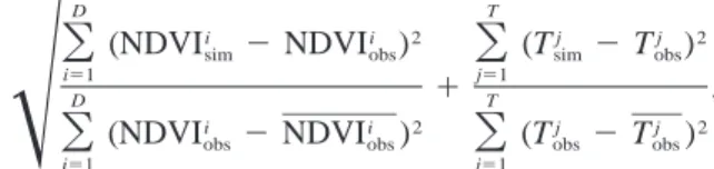
and S1, respectively). These results do not change when simulation S4 is iterative. The vigor parameter and soil resistance coefficients stabilize at 1.34 and 8300/1900. Similar results are obtained when all these parameters are calibrated simultaneously using the following cost function
D T
i i 2 j j 2
(NDVI 2 NDVI ) (T 2 T )
O
sim obsO
sim obsi51 j51
1 ,
D T
Î
O
(NDVIi 2 NDVI )i 2O
(Tj 2 T )j 2obs obs obs obs
i51 j51
(Tjis the radiative temperature, D and T are the number
of observations, the indices ‘‘sim’’ and ‘‘obs’’ refer to simulated and observed, respectively). Thus, our con-clusions seem to be robust.
2) SATELLITE THERMAL INFRARED DATA
Table 5 presents the AVHRR surface temperature ob-tained with a split window technique (Kerr et al. 1992), along with the ground measurements of brightness tem-perature (emissivity is 1) for the same sites and the same hours. It also shows the brightness temperature esti-mated by the V–S model, [Eq. (1)], that was calibrated with AVHRR shortwavelength data (S2 simulations) on the three sites. The model therefore has realistic vege-tation dynamics. Because of cloud contamination and view angle restriction, the number of afternoon AVHRR scenes with coexistent ground data is low. Table 5 shows that the AVHRR temperature is significantly lower than the simulated brightness temperature. On the CES, dif-ferences of 58 are common during the growing season. The difference is larger when the emissivity is consid-ered. As shown by van de Griend et al. (1991), thermal infrared emissivities (8–14mm) of natural surfaces with-in the savanna environment may vary between 0.914 for bare soil and 0.986 for a vegetated surface. The corresponding surface temperatures are 6 and 1 K higher than the brightness temperature, respectively, for a brightness temperature around 300 K.
Not surprising, this difference between AVHRR tem-perature and simulated brightness temtem-perature has a large impact on the calibration scheme, even if a very high emissivity is assumed. An adjustment of the soil resistance parameters was performed to match the AVHRR surface temperature after the plant vigor had been calibrated with AVHRR NDVI time series. No emissivity correction was applied to the AVHRR surface temperature, so the difference between modeled and measured temperature is underestimated. Because the model attempts to drastically cool the surface, the cal-ibration leads to unrealistic parameters values. As a
re-sult, the calibration of the vegetation–SVAT model with AVHRR surface temperature data was unsuccessful at this stage. Some reasons for these discrepancies are dis-cussed in the following section.
6. Discussion
This study describes the first attempt to calibrate a V–S model with satellite shortwave and longwave data over several uncultivated vegetation sites. This meth-odology produced several interesting results and is suit-able to address upscaling problems for surface fluxes and vegetation growth modeling. On the other hand, it also pointed out some difficulties in using satellite long-wave data. Among the more interesting results was the ability to constrain the V–S model using shortwave sat-ellite data. Similar conclusions were obtained with crop-growth models (Moulin et al. 1998). However, crop models benefit from numerous control studies that sim-ply do not exist for natural vegetation. It was therefore important to establish the suitability of the calibration methodology in the case of natural vegetation. These results also showed that modeling of the canopy short-wave radiative properties (NDVI) with the SAIL model is robust and can be applied to multispecies sparse can-opies. The results obtained with airborne and satellite shortwave data were similar. This shows that the data processing, the heterogeneity treatment (linear unmix-ing), and the links between LAI and NDVI are accurate enough to make full use of operational sensors and data streams. One should note that the initial conditions for growth had to be prescribed in this study, especially for the CWS and SS. Therefore, the ability to constrain the phenology (i.e., growth timing) could not be completely assessed. Yet, phenology may also be a good candidate for calibration (Kergoat et al. 1995a; Moulin et al. 1997). Reducing the number of parameters, as we did for the vegetation ‘‘vigor,’’ should allow us to constrain both vigor and phenology with NDVI time series. The second interesting result was that the simulation of the surface fluxes was fairly good (rmse for heat latent flux on the grassland CES is 60 W m22), once the V–S model
had been calibrated from satellite shortwave data. In particular, the simulation of the site-to-site variability was greatly enhanced by the calibration procedures. As-similating shortwave satellite data into a V–S model appears to be particularly suited to assess the water and energy exchanges at the regional scale, as well as their seasonal variations.
The use of radiative temperature was less successful. We showed that some parameters that are directly related to the energy balance could be calibrated with ground-based brightness temperature measurements. However, this further calibration did not add much to the simu-lation of surface fluxes. Two different reasons could explain this result: (a) the NDVI data may possess a ‘‘better’’ information content, or (b) this may simply reflect the greater sensitivity of the fluxes to the LAI
FIG. 10. Comparison of the LAI time profile measured over the CES grassland (asterisks) with the V–S simulations. The dotted line is the reference simulation (simulation S0), and the solid line is the LAI simulation after V–S calibration with ground-based radiative temperature data (simulation S5).
calibration than to the resistance parameters. To assess further these questions, we performed a calibration of the vegetation vigor parameters V using the ground TIR data instead of the NDVI (simulation S5, V5 1.2 with a confidence interval at 95% of [0.96, 1.43]). As shown by Fig. 10, this calibration improved the LAI simulation, as compared with the a priori S0 case for the CES. It also improved the simulation of the latent heat flux and radiative temperature (Table 3, simulation S5). Indeed, using either ground-based TIR or NDVI data lead to very similar results. The conclusion of this test is that the TIR data also contains ‘‘useful’’ information. Al-though both NDVI and TIR data were suitable to con-strain the V–S model, the synergy between the two wavelengths was not clearly demonstrated. The main reason for that is the high sensitivity of the V–S model’s temperature and fluxes to vegetation cover. This con-clusion is probably valid for semiarid areas only, where vegetation development and soil moisture are highly correlated on a seasonal basis [see Ottle´ and Vidal-Mad-jar (1993) for a different case].
The last insight was that satellite longwave data proved unsuitable for model calibration at this stage. The AVHRR surface temperature values were found to be much lower than the ground-based measurements over the grassland sites, and this brings into question the temperature retrieval algorithm. Based on very lim-ited datasets over some HAPEX-Sahel subsites, the split window algorithm used in this study was favorably com-pared to other algorithms by Andersen et al. (1997), whereas Caselles et al. (1997) suggested that it could
underestimate surface temperature by 3.58. Indeed, com-parison between satellite data and ground data is often a challenge in itself. This is particularly true for the AVHRR over land. As noted by Kerr et al. (1998) and Zhihao Qin and Karnieli (1999), the main problems for comparison can be summarized as follows:
R It is difficult to assess the emissivity values to correct
the ground measurements.
R The AVHRR sensor and the radiometers used for
ground measurements have different spectral respons-es.
R The pixels are not pure and the ground data
repre-sentativeness may be questioned. Unlike in the red and near-infrared bands, the linear unmixing method cannot be applied to the AVHRR surface temperature measurements because the assumption that each veg-etation type shows the same surface temperature over contiguous pixels does not hold.
R The difference in the acquisition time at the ground
and satellite level can be a major source of error sec-ond to the heterogeneity problem.
For all these reasons, it is extremely difficult to compare ground measurements and satellite data. As a result, the interpretation of remotely sensed longwave data has not reached the same maturity that the interpretation of shortwave data has. The results from the FIFE experi-ment lead to similar conclusions (Schmugge and Schmidt 1998). In that case, the spatial heterogeneity was also the best candidate to explain the discrepancies. The use of differential measurements of surface tem-perature may circumvent some of the measurement problems. For example, the diurnal cycle provided by
GOES-8 and future Meteosat second-generation may
help to constrain SVAT (Jones et al. 1998a) or V–S models, even in the presence of systematic biases be-tween modeled- and satellite-derived temperatures. In this study, the results based on ground data established that there is potential to use the temperature measure-ment in conjunction with V–S models. In comparison with the shortwave data, there is more room for im-proving the satellite-based algorithms.
7. Conclusions
This study presented a coupled vegetation–SVAT model (V–S model) and investigated the feasibility in calibrating the V–S model with ground-based, airborne, and satellite data in the shortwave and longwave do-mains. The coupled vegetation–SVAT model was de-scribed and calibrated using ground data collected over three semiarid grassland sites during the HAPEX-Sahel experiment. A sensitivity analysis showed that the pa-rameters related to plant growth vigor and to soil evap-orative resistance were the best candidates for calibra-tion. The radiative temperature is equally sensitive to the vegetation parameters and to the water and energy parameters (i.e., the vegetation cover has considerable
effect on radiative temperature). This emphasizes the importance of the accuracy of LAI simulation. The im-pact of calibrating model parameters with time series of AVHRR normalized vegetation index and thermal infrared data was assessed by examining the simulations of latent heat flux and LAI for a suite of calibration experiments. The results showed that both airborne and AVHRR NDVI data can be used to constrain the V–S model. These constraints significantly improved the simulations of the LAI and latent heat flux. In particular, the site-to-site variability was greatly enhanced by the calibration procedures. The model can also be calibrated with ground-based radiative temperature data. Although both NDVI and temperature data were suitable to con-strain the V–S model, the synergy between the two wavelengths was not clearly demonstrated. Moreover, satellite surface temperature data proved unsuitable for model calibration at this stage. The AVHRR surface temperature values were found to be much lower than the ground-based measurements over the grassland sites. Therefore, the best simulations of LAI and latent heat flux were obtained by constraining the V–S model with NDVI satellite data; the main reason was that the re-lationships between the satellite signal and the surface variables seem to be more robust in the short-wave do-main than in the thermal infrared dodo-main. The use of satellite thermal infrared still requires further work to alleviate the challenging heterogeneity and accuracy problems. As a conclusion, we think that the calibration of a coupled vegetation growth–SVAT model (V–S) with shortwave satellite data can now be used to im-prove the simulation of the seasonal and spatial vari-ability of the surface energy and water exchanges. This approach may be used to address the scaling of the surface fluxes up to the regional scale.
Acknowledgments. This work was made possible
through a Ph.D. grant from French MESR (Ministe`re de l’Enseignement Supe´rieur et de la Recherche), the support of the European Commission to the Vegetation Preparatory Program, and of the Fourth Environment and Climate Program. The authors wish to express their sincere gratitude to the HAPEX-Sahel Information Sys-tem at CESBIO. Yann Kerr is gratefully acknowledged for stimulating discussions. Special thanks are due to the many people involved in the implementation of the experiment, particularly to Drs. B. A. Monteny, S. D. Prince, N. P. Hanan, and P. E. Levy. The authors also thank Cristina Kaufman for carefully reading and ed-iting the manuscript. We would like to thank gratefully the anonymous reviewers for their constructive criti-cism.
APPENDIX A
Description of the Coupled Vegetation–SVAT Model
a. Water and energy balance submodel
The SVAT model presented in this paper describes the major land surface water and energy exchange
pro-cesses between the biosphere and the atmosphere. The surface is represented using the two-sources approach proposed by Shuttleworth and Wallace (1985). Soil and vegetation contributions to sensible and latent heat flux-es are explicitly parameterized. The incoming solar ra-diation is partitioned between bare soil and vegetation through a screen factorsf(i.e., Deardorff 1978; Taconet
et al. 1986). The shielding factor sf is expressed as a
function of the LAI following Beer’s law: sf 5 1 2
exp(0.4LAI). Note that variables are defined in Appen-dix B. The energy balance, written separately for the soil and the vegetation, gives
Rns2 LE 2 H 2 G 5 0 ands s (A1)
Rnc2 LE 2 H 5 0,c c (A2)
where Rn is the net radiation, LE is latent heat flux, H is sensible heat flux, G is ground heat flux, and the indices s and c refer to soil and canopy, respectively.
The network of resistances from Shuttleworth and Wallace (1985), between the soil surface, the within-canopy source level, and the above-within-canopy reference level allows estimation of the latent and sensible heat fluxes through differences in vapor pressure and in tem-perature: rC e 2 ep o a LE5
1
2
and (A3) g raa rC (T 2 T )p 0 a H5 . (A4) raaFor the soil component:
rC e (T ) 2 ep sat g o LEs5
[
]
and (A5) g ras 1 rss rC (T 2 T )p g o Hs5 . (A6) rasFor the vegetation component:
rC e (T ) 2 ep sat c o LEc5
[
]
and (A7) g rac 1 rc rC (T 2 T )p c o Hc5 . (A8) racThe resistance formulations are found in appendix C, except for the canopy resistance (rc), which is detailed
in appendix Ab(3).
The volumetric soil water content of ground surface (wg) and of roots layer (w2) result from the water
bal-ance, which is based on the force–restore approach de-veloped by Deardorff (1978) and adapted by Noilhan and Planton (1989):
]wg C G1 C2 5 (P2 E ) 2g (wg2 w )eq ]t r dw 1 t when 0, w # wg fc (A9) and (P2 E 2 E ) ]w2 g tr 5 when 0, w # w . (A10)2 fc ]t r dw 2
b. Vegetation growth submodel
The vegetation model aims at simulating the time evolution of three compartments: the shoots biomass, (Ms), the roots biomass, (Mr), and the standing
necro-mass, (Mn). The main processes that drive these three
variables are photosynthesis, allocation of photosyn-thates to both shoots and roots, respiration, and senes-cence. The overall structure of this vegetation model is similar to some crop growth or grassland models (e.g., Spitters et al. 1989; Mougin et al. 1995; Lo Seen et al. 1995; Nouvellon 1999). The canopy gas exchange scheme, that is, stomatal and canopy resistance and pho-tosynthesis, has been used for various biomes, and is described in Kergoat (1998).
1) CARBON BALANCE
The dynamics of the three carbon compartments are described by a set of differential equations:
dMs 5 a Pn 2 m M 2 Rg 2 s M ,s s s s s s (A11) dt dMr 5 (1 2 a )Pn 2 m M 2 Rg 2 s M , and (A12)s r r r r r dt dMn 5 s M 2 d M .s s n n (A13) dt
Equation (A11) expresses that the daily carbon incre-ment of the shoots is the result of the carbon gain [pho-tosynthesis, Pn, minus the carbon losses (respiration and senescence: ssMs)]. Plant respiration consists of the
maintenance (ms, Ms) and growth respiration (Rgs). The
carbon fixed through photosynthesis is partitioned be-tween the shoots and roots according to the allocation coefficient (as). The roots obey a similar equation [Eq.
(A12)], with a symmetric allocation coefficient (1 2
as). The necromass dynamics depend on the difference
between necromass production, which is equal to the shoots senescence, ssMs, and necromass decay, dnMn.
The LAI is computed from the shoots biomass ac-cording to a nonlinear relationship that accounts for the increasing importance of stems and other nonleaf tissues at high levels of biomass [empirical relationship, e.g., Le Roux (1995)] by the expression
LAI5 SLA0[12 0.48(1 2e225.5Ms)]Ms, (A14)
where SLA0is the specific leaf area for low levels of
the shoots biomass.
The carbon balance equations [Eqs. (A11)–(A13)] are solved on a daily basis, whereas the photosynthesis (Pn) is computed and accumulated on an hourly basis. In-deed, it depends on the stomatal resistance, which is also involved in the SVAT model, and computed on an hourly basis.
2) CARBON POOLS INITIALIZATION
For the annual vegetation considered in this study, the shoots and roots compartments are initially empty at the beginning of the rain season. Model initialization consists of using a prescribed amount of carbon, which represents the seeds that germinate, to grow the first leaves and roots. This process is parameterized using an initial amount of carbon and a daily rate at which this carbon is injected into the two compartments (IC and Trans parameters in appendix B). For two sites (CWS and SS), the meteorological data during the first part of the growing season were not available. There-fore, the shoots biomass was initialized to correspond to the biomass field measurements for the first day of the simulations (Day 231 of 1992 for CWS and SS). Moreover, as the simulations do not really extend into the dry season, the necromass decay was neglected (dn set to 0, appendix B). For the CES site, the start of the growing season (germination) was set to day of year (DoY) 180.
3) PHOTOSYNTHESIS AND RESISTANCE SCHEME
The vegetation model uses a scheme that accounts for the response of canopy photosynthesis to soil and atmosphere forcing. At an hourly time step, a leaf level photosynthesis model is integrated to the canopy level according to canopy LAI. The rate of leaf photosyn-thesis, Pl, is given by
Ca2 G
Pl5 , (A15)
rs1 rr
where Ca 2 G is the difference in CO2concentration
between the chloroplast and the atmosphere; rs and rr
are the stomatal and residual resistances to CO2transfer
(e.g., Running and Coughlan 1988). The stomatal re-sistance is a Jarvis type rere-sistance (Jarvis 1976), where a minimum resistance, rsmin, is increased according to
stress factors, rs5 rs minf (I )g(w )h(VPD)2 w 2 w Is1 I fc wp40002 1000 5 rs min , (A16) I w22 w 4000 2 VPDwp
where I and Isrepresent the incoming Photosynthetically
Active Radiation (PAR) and the PAR level for stomata half-closure (Saugier and Katerji 1991), respectively; here, w2 is the soil moisture content of the root zone;
and wwp and wfc are the soil moisture at wilting point
and at field capacity, respectively. The term VPD is the water vapor deficit (Pa).
Photosynthesis biochemistry is represented by the g1
and g2 factors in the residual resistance equation and
accounts for PAR and temperature effects (Running and Coughlan 1988), rr5 rr ming (I )g (T )1 2 2 Ir1 I (Tmax 2 T )min 5 rr min , (A17) I 4(Tmax 2 T)(T 2 T )min
where T is the air temperature.
For both resistances [Eqs. (A16) and (A17)], the light factors are simple analytical functions, which ensure a classical hyperbolic light response of leaf photosynthe-sis, P1, versus PAR, in the absence of stresses. The
parameters for the residual resistance, rrmin and Ir, are
calibrated according to Eqs. (A18) and (A19) to match literature values for the maximum rate of photosynthe-sis, Pmax [Eq. (A18)], and the quantum yield, a [Eq.
(A19)]:
Ca2 G
Pmax 5 and (A18)
rs min1 rr min
Ca2 G
a 5 . (A19)
(rs min sI 1 rr min rI )
The minimum stomatal resistance, rsmin, comes from
ground measurements of Hanan et al. (1997). This pho-tosynthesis scheme reproduces the main features of plant photosynthesis response, that is, the effects of PAR, soil water, air temperature, water vapor deficit, and seasonal variations. Combined with a classical Beer’s law for light extinction in the canopy, this leaf level model leads to an analytical expression when in-tegrated to the canopy level:
LAI Pc5 tp
E
P dL1 0 i.e., t (Ca 2 G)p Pc5 k (re s9 1 r9)r r9I 1 r9I 1 k I (r9 1 r9)s s r r e 0 s r 3 ln ,rs9I 1 r9I 1 k I (r9 1 r9) exp(2k LAI)s r r e 0 s r e
(A20) where Pcis the hourly canopy photosynthesis, I0is the
incoming PAR at the top of the canopy,tpis the SVAT
time step, keis the extinction coefficient for PAR in the
canopy; r9s is for rsming(W )h(VPD), and r9r is for
rrming2(T ). The hourly canopy photosynthesis, Pc, is
ac-cumulated to produce the daily photosynthesis (Pn) used in Eqs. (A11) and (A12).
The canopy resistance for water vapor diffusion, rc,
which is used by the SVAT submodel, is also given by an analytical formula: LAI 1 1.6 5
E
dL rc 0 rs 1 1.6 Is1 k Ie 0 i.e., 5 ln , (A21) rc k re s9 I 1 k I exp(2k LAI)s e 0 ewhere 1.6 is the ratio of the CO2and water vapor
dif-fusivities.
4) RESPIRATION AND SENESCENCE
Following McCree (1970) and Amthor (1986, 1989), the total respiration consists of maintenance and growth respirations. The maintenance respiration is proportion-al to the biomass and its rate [msor mrin Eqs. (A11)
and (A12)] depends on air temperature according to a classical Q10 relationship:
ms5 ms0Q10T/10, (A22)
where T is the daily average air temperature and ms0
(mr0) is the respiration rate at 08C for the shoots (roots).
The growth respiration is proportional to the amount of new tissues and therefore Eqs. (A11) and (A12) are rearranged as follows: dMs 1 5 (a PNs 2 m M ) 2 s M ands s s s (A23) dt 11 gs dMr 1 5 [(1 2 a )PN 2 m M ] 2 s M , (A24)s r r r r dt 11 gr
where gs(gr) is the amount of carbon released by growth
respiration per unit of new shoots (roots) tissue. Typical values for the respiration parameters were taken from Amthor (1989). Last, the dry matter is lost through the senescence of shoots and roots tissues [Eqs. (A23) and (A24)]. We considered here a senescence rate, ss0, (sr0
for roots) and a water stress effect that increases se-nescence: s Ms s5 s f (w )Ms0 2 s w22 wwp 5 s 1 1 1 2s0
[
1
2
]
M .s (A25) wfc2 wwp APPENDIX BVariables, Parameters, and Constants Used in the Vegetation–SVAT Model
Symbol Definition Type
Ca2 G CO2concentration gradient
be-tween leaf surface and chloro-plast (Ca2 G 5 0.640 g CO2
m23)
Parameter
Cp Specific heat at constant pressure
(J kg21K21)