HAL Id: inserm-00250168
https://www.hal.inserm.fr/inserm-00250168
Submitted on 11 Feb 2008
HAL is a multi-disciplinary open access
archive for the deposit and dissemination of
sci-entific research documents, whether they are
pub-lished or not. The documents may come from
teaching and research institutions in France or
abroad, or from public or private research centers.
L’archive ouverte pluridisciplinaire HAL, est
destinée au dépôt et à la diffusion de documents
scientifiques de niveau recherche, publiés ou non,
émanant des établissements d’enseignement et de
recherche français ou étrangers, des laboratoires
publics ou privés.
high-dimensional data.
Sylvain Lespinats, Michel Verleysen, Alain Giron, Bernard Fertil
To cite this version:
Sylvain Lespinats, Michel Verleysen, Alain Giron, Bernard Fertil. DD-HDS: A method for
visualiza-tion and exploravisualiza-tion of high-dimensional data.. IEEE Transacvisualiza-tions on Neural Networks, Institute of
Electrical and Electronics Engineers, 2007, 18 (5), pp.1265-79. �inserm-00250168�
Abstract— Mapping high-dimensional data in a low-dimensional space, for example for visualization, is a problem of increasingly major concern in data analysis. This paper presents DD-HDS, a nonlinear mapping method that follows the line of Multi Dimensional Scaling (MDS) approach, based on the preservation of distances between pairs of data. It improves the performance of existing competitors with respect to the representation of high-dimensional data, in two ways. It introduces i) a specific weighting of distances between data taking into account the concentration of measure phenomenon, and ii) a symmetric handling of short distances in the original and output spaces, avoiding false neighbor representations while still allowing some necessary tears in the original distribution. More precisely, the weighting is set according to the effective distribution of distances in the data set, with the exception of a single user-defined parameter setting the trade-off between local neighborhood preservation and global mapping. The optimization of the stress criterion designed for the mapping is realized by "Force Directed Placement". The mappings of low- and high-dimensional data sets are presented a s illustrations of the features and advantages of the proposed algorithm. The weighting function specific to high-dimensional data and the symmetric handling of short distances can be easily incorporated in most distance preservation-based nonlinear dimensionality reduction methods.
Index Terms — high-dimensional data, neighborhood visualization, non-linear mapping, Multi Dimensional Scaling.
I. INTRODUCTION
isualization of high-dimensional data is intended to facilitate the understanding of data sets by preserving some "essential" information. It generally requires the mapping of the data into a low (usually 2- or 3-) dimensional space. However, high-dimensional data raise unusual problems of analysis, given that some properties of the spaces they live in cannot be extrapolated from our common experience. In particular (notably in the case of Euclidian spaces), we often face the problems of empty space and concentration of measure: when the number of dimensions is high, the neighborhood of each object is
Manuscript received December 28, 2005, accepted in 14 December 2006. This work was supported in part by the Action INTER EPST Bio-informatique 2001 Grant, contract N° 120910.
S. Lespinats, A. Giron and B. Fertil are with the UMR INSERM unité 678 - Université Pierre et Marie Curie-Paris 6;, boulevard de l'hôpital, 75634 Paris. France (corresponding author phone: 0033 (0) 1 53 82 84 07; fax: 0033 (0) 1 53 82 84 46; e-mails: [email protected] ,
[email protected] , [email protected] ).
M. Verleysen is with Université catholique de Louvain, 3, place du Levant, B-1348 Louvain-la Neuve (Belgium) and SAMOS-MATISSE, Université Paris 1 Panthéon-Sorbonne, 90 rue de Tolbiac, 75634 Paris Cedex 13 (France); e-mail: [email protected]
scarcely filled whereas most of the other objects are found in a thin outer shell. Distances between high-dimensional objects are usually very concentrated around their average [1].
Exploration and analysis of high-dimensional data are often made by means of dimension reduction techniques [2, 3]. Since human experience mostly deals with three-dimensional space (and most data display devices are two-dimensional), finding a meaningful mapping of high-dimensional data into such low-high-dimensional spaces is a major issue. Often linear mapping methods do not lead to satisfactory representations. Indeed real data most often show nonlinear relationships that cannot be approximated in a satisfactory way by linear methods. Nonlinear mappings (also called nonlinear methods for dimensionality reduction) offer more flexibility, often at the price of an additional complexity.
In this paper, we propose a nonlinear dimensionality reduction method specifically adapted to high-dimensional data. It follows the line of Multi Dimensional Scaling (MDS) methods, based on the preservation of distances between pairs of data [4]. However, it differs from existing methods in two ways. First, it includes a weighting of distances that takes the concentration of measure phenomenon into account (see section IV.A); this is of primary importance when dealing with high-dimensional data, for which the concept of "small" and "large" distances strongly differ from the traditional view in low-dimensional spaces. Secondly, existing nonlinear dimensionality reduction methods either favor the preservation of small distances in the original space ([5] for example), at the risk of collapsing far points together in the representation, or favor the preservation of small distances in the output space ([6] for example), allowing sometimes unwanted tears in the original distribution. The method proposed in this paper is symmetric with respect to distances in the original and output spaces (see section IV.B), leading to better and more intuitive representations, as attested by experiences. Finally, the optimization of the method-specific objective function is performed by Force Directed Placement (FDP), as an alternative to more traditional gradient-based algorithms (see section IV.C).
This paper is organized as follows. Section II shows known phenomena occurring in high-dimensional spaces, and how metric transformations can deal with them. Section III briefly reviews dimensionality reduction methods, and highlights the difficulties encountered in these methods with high-dimensional data. Section IV presents our original nonlinear mapping algorithm called DD-HDS for Data
DD-HDS: a method for visualization and
exploration of high-dimensional data
Sylvain Lespinats, Michel Verleysen, Senior Member, IEEE, Alain Giron, Bernard Fertil
Driven High-Dimensional Scaling. Section V defines efficiency measures used in section VI that presents experimental results and comparisons with existing methods.
II. DISTANCES IN HIGH-DIMENSIONAL SPACE
Mapping methods based on the comparison of distances between pairs of data in the original and output spaces, such as MDS, need to take care of how distances are measured. Specific distances are often used to measure similarities in the original space; distances in the (low-dimensional) output space are usually measured in a more conventional way. In this paper, we focus on Euclidean and derived metrics (section II.A and section II.B, respectively) for the representation of data in the original space and on the Euclidean metric for the output space for sake of simplicity. However, most results in this work may be easily extended to other metrics.
A. Euclidean distances in high-dimensional space
Several surprising phenomena appear when dealing with high-dimensional data. This fact is known as the "curse of dimensionality" [1], and has strong impact on the validity and performances of data analysis tools [7]. In particular, the Euclidean metric ( x =
∑
xi2) is known to suffer from theunwanted concentration of measure phenomenon [8]. Let us consider the distances between pairs of uniformly distributed data in a n-dimensional unit-edge hypercube. It can be shown that the mean of the distances increases with the square root of n, while the variance remains constant. This is illustrated in Fig. 1. As a result, it is much more difficult to discriminate between small and large distances in a relative way (e.g. when distances are normalized) in a high-dimensional space. As we will see in a short review in the next section, nonlinear dimensionality reduction tools will thus fail to give more weight to small and/or large distances, as it should be the case for a proper functioning of the algorithms.
The Euclidean norm is not the only one to suffer from the concentration of measure phenomenon. All other Minkoswki metrics, Minkowski pseudo-metrics (fractional norms), Pearson correlation metric, etc… have this characteristic, though at different levels [8]. Transformations of distances may be used to overcome these problems. We briefly review such transformations in the next subsections.
B. Derived metrics
It is common practice changing data representation to help the mapping procedure and, eventually, to add supervised information (see [9] for example). Three powerful approaches are particularly useful as preprocessing when dealing with high-dimensional data.
1- Nowadays kernel methods have a huge attractiveness in data analysis [10]. Kernel methods rely on the principle of first mapping data onto a (usually higher-dimensional) space before further processing. In practice, the mapping is not explicitly calculated: a so-called kernel k(.,.) is used to calculate distances between the mapped data. If the kernel is positive definite, it can be verified that it is indeed the scalar product between data in a transformed space: k(xi,xj)=
<φ(xi), φ(xi)> where <. , .> denotes the scalar product and
φ(.) a mapping to a possibly high-dimensional space. The so-called kernel trick avoids calculating both the mapping and the distances (here scalar products) in the original spaces: only the outputs of kernels have to be evaluated.
By using nonlinear transformations of data, kernel methods succeed in building nonlinear models (e.g. for classification and regression) keeping many advantages of linear tools. Their optimization procedure is also simplified compared to many other nonlinear models.
Kernels are used in the context of nonlinear dimensionality reduction too. This leads for example to the Kernel Principal Component Analysis (KPCA) method consisting in applying the linear PCA method in a kernel-induced space [10-13]. As kernels are defined as a dot product between nonlinear data transformations, Kernel PCA can be viewed as PCA applied after a transformation of metric. As in MDS methods, the user is faced to the crucial choice of an adequate metric transformation, more precisely to the choice of the kernel [11, 14]. Weinberger et al. for example use semidefinite programming for manifold learning that provides optimized kernels for high-dimensional data projection [15, 16]. In this context, it must be pointed out the high similarity of this approach with Fast Mixing Markov chains [17]. A variant, described in [10] page 436, consists in using classical MDS on a distance matrix generated through a kernel function. Taking the exponential of (Euclidean) distances is a possible transformation that enhances the contrast between small and large distances.
dim=1
dim=2
dim=5
dim=10
dim=20
dim=50
dim=200
0
0
distance
count
5
10
15
20
25
Fig. 1. Histogram of distances between uniformly distributed data in a unit cube, according to space dimension. Histograms for dimensions larger than 200 would have the same Gaussian-like shape, but their centers would be shifted to the right proportionally to the square root of the dimension.
2- Geodesic metrics (also called curvilinear metrics) may offer interesting data representations when dealing with high-dimensional spaces. They are based on the fact that if data occupy a non-convex part of the space, it seems legitimated to force distances to be measured through the cloud of data, instead of using a conventional Euclidean distance. Intuitive justifications for the interest of curvilinear distances may for be found for example in [18, 19]. The curvilinear distance is measured in a graph the nodes of which are the data themselves (or a reduced set). Close data in the space are linked together to form a connected graph (the way they are connected define the type of distance; classically, each node is connected to the k closest nodes). The curvilinear distance between any pair of data xi and xj is
subsequently the sum of Euclidean distances between all pairs of data connected in the shortest path on the graph between xi and xj.
Floyd's and Dijkstra algorithms may be used to compute such distances [20, 21]. Isomap [18] and Curvilinear Distance Analysis (CDA) [19, 22] are methods belonging to this category, the difference resulting in the way distances are weighted: Isomap extends classical MDS [4] while CDA extends the "Curvilinear Component Analysis" [6]. Extensions to these methods have been published, e.g. to allow the possibility for tears in the original distribution, avoiding loops or other closed surfaces to collapse in the mapping (see for example [23]).
3- A last class of derived metrics discussed here consists in using rank orders. Indeed on some data (such as genomic signatures [24]), the ranking of neighbors is important, while the distance itself may be less [25]. Switching from distance to rank order may thus reveal interesting data properties. Kruskal's criterion is close to such a transformation [26, 27].
Rank orders are not symmetric: let’s note
X= x
(
1, x2,..., xN)
the data in the original space; if data xi isthe k-th neighbor of xj, xj is not necessarily the k-th neighbor
of xi. In order to use the rank as a distance,
d
ijr
may be defined as the average of the rank order of xi with respect to
xj and vice-versa. Note that, nevertheless,
d
r
must be called a pseudo-distance as it is does not respect the triangular inequality. Furthermore this pseudo-distance is data set dependent (just as curvilinear distance is), as
d
ijr may be influenced by the addition of a data xk (k ≠ i and k ≠ j) inthe data set; to limit this effect, it is possible to normalize the pseudo-distances (for example by their maximum value). By construction, rank orders do not suffer from the concentration of measure phenomenon; however, they are not commonly used in nonlinear dimensionality reduction methods, probably due to the lack of conventional distance properties.
All these derived metrics are designed to enhance the contrast between small and large distances. However, whatever is the method used for that purpose, they fail to address the specific properties of high-dimensional data. The concentration of distances phenomenon detailed in section II.A makes that all distances are approximately equal. Transforming these distances by a nonlinear function such a kernel does not help, unless the transformation is designed specifically to take the concentration phenomenon into
account. This is the goal of the algorithm described in section IV.
III. DIMENSION REDUCTION TECHNIQUES
Data X = x
(
1, x2,..., xN)
are defined in the vector space E1with associated metric m1. Our goal is to represent X in a vector Euclidian space E2 of lower dimension than N.
Mapping data from a high-dimensional space to a low-dimensional one, keeping exactly all distances between the pairs of points in the original and output spaces, is most often impossible whatever is the distance used to measure similarities in the original space. Then, a data representation has to release some constraints according to a specific “point of view”. Numerous dimensionality reduction methods have been proposed, with variants in the methodology and in the criterion (the point of view) to optimize. In this section, we briefly present the main aspects of these techniques, before providing some insight about the difficulties encountered when the dimension of the original space is high.
A. Approaches for dimension reduction
Because keeping exactly all distances between pairs of points unchanged in the representation is most often impossible, all methods emphasize the preservation of some distances or types of distances, therefore privileging a specific point of view. For example, Principal Component Analysis (PCA) and classical MDS [4, 28, 29] maximize the variance of the data cloud after projection, under linear projection hypothesis; the resulting representation expresses the overall form of the data set. Locally Linear Embedding (LLE) [30], Laplacian Eigenmaps [31] and Hessian-based Locally Linear Embedding (HLLE) [32] assume that data are located on a manifold, smooth enough to be reasonably well approximated by local linear models ; these methods unfold the set of data through local linear projections. The merging of local projections may be optimized afterward [33]. Supervised methods such as Discriminant Analysis and Partial Least Squares (PLS) regression [34] use a dependent variable (discrete or continuous, respectively) to guide the mapping. Self-Organizing Maps (SOM) [35, 36] visualize data on a grid obtained by a topology-preserving vector quantization. ViSOM and PRSOM merge SOM and MDS algorithms in order to map data based both on topology and distance preservation [37-39]. The Generative Topographic Mapping (GTM) is also inspired from SOM [40]: a lower-dimensional manifold is optimized to approach data in the original space (see [41] for discrete data). The Gaussian Process Latent Variable Model (GP-LVM) results from a novel probabilistic interpretation of PCA [42]. This non-linear method is close to KPCA and GTM. Methods such as Sammon’s mapping [5], non linear MDS [26, 27, 43], Curvilinear Component Analysis (CCA) [6, 44], and Isotop (a SOM the nodes of which are positioned by CCA) [45, 46] emphasize on local neighborhood preservation, often at the price of allowing huge deformations of the global shape of the data cloud. Note that the CCA acronym used in this paper according to the literature covering this algorithm does not mean here Canonical Correlation Analysis. As detailed in the previous section, derived distances in the original space may be used, entitling for example the use of MDS after a kernel transformation, or the replacement of Euclidean
distances by curvilinear distances in MDS and CCA, leading to Isomap and CDA respectively.
The method introduced in the next section is placed in the context of neighborhood preservation. The goal is to build a method emphasizing on the preservation of small distances, possibly at the price of distortions in large distances. The difference with respect to previously mentioned methods arises from the fact that the specific properties of high-dimensional spaces are taken into account when measuring distances in the original space. Furthermore, the question whether to emphasize on small distances in the original or output space is answered in a symmetric way, offering a compromise between the risk of mapping far points together and the possibility to tear the initial distribution for a better representation.
B. Sammon’s stress and high-dimensional data
Distance preservation methods such as Sammon's mapping, CCA and CDA, minimize the differences between
di j, the distance between xi and xj in the original space, and
d'i j, the distance between their representations x'i and x'j in
the output space. Small distances are emphasized in order to preserve local topology (and small distances). An objective criterion
ς
=
F d
(
ij− ′
d
ij.
k d
( )
ij)
i< j
∑
similar to the originalSammon's stress, where k(di j) is a monotonically decreasing
function giving more weight to small distances in the F criterion is generally used. Sammon's stress [5] is for example :
ς
sammon=
1
d
ij i< j∑
(
d
ij− d'
ij)
2d
ij i< j∑
, (1)and Kruskal criterion [27] is:
∑
<−
=
j i ij ij ijd
d'
d
2 2 kruskal'
)
(
ς
. (2)Stress functions as (1) and (2) are also called error functions, energy function or loss functions, depending on the literature.
In both cases, the weighting function is related to the inverse of the distance. In high-dimensional spaces however, as detailed in section II.A, all distances tend to be similar. The weighting factor in (1) and (2) does not play its role anymore. The criterions then give similar weights to small and large distances, leading to a mapping that mixes global representation and local neighborhood preservations. Such a poor behavior of Sammon's stress was already mentioned by its author, who noted that linearly separable classes in high-dimensional spaces might not be separable in the mapping [5].
C. Representation with false neighborhoods or tears
Distance preservation methods penalize more heavily mismatches in small distances, by weighting the stress criterion with a decreasing function of either the distances in the original space (see (1) for example), or the distances in the output space (see (2) for example). However, in the first case, it is difficult to tear distributions with loops, leading to the so-called "false neighborhood" representation: data far from each other in the original space could be mapped to
close points, exactly as PCA "flattens" volumes when the number of principal components used in the projection is not sufficient. As an example, the extreme points of a "C" shape (two-dimensional space) with two long branches (with respect to their inter-distance) will be projected as neighbors (in a one-dimensional space), although their distance in the original space is large (compared to distances between neighbouring points in the "C" shape); a good mapping procedure would unroll the "C" shape instead of flattening it.
In the second case, tears are allowed, with the risk that neighbor points in the original space may be found widely separated in the output space; tears are sometimes necessary, but may lead to wrong interpretations of neighborhoods in the output space. For example, mapping a "O" shape requires tears to avoid flattening and false neighbors, but the location of tears appears randomly in some methods, or depends more strongly on the density of data in the original space than on the manifold geometry.
False neighbors and tears are limitations of nonlinear dimensionality reduction methods, which cannot be avoided in most cases due to the intrinsic nature of the manifold. Illustrations of tears and false neighbors are provided in section VI.E, where mappings of open boxes with various algorithms are shown.
However, in most cases, there is no reason to favor a
priori false neighbors or tears. See the recent paper of
Lawrence and Quiñonero-Candela for a comprehensive discussion of this problem in terms of similarities and dissimilarities between data [47]. There is thus a need for a method that implements a compromise and reduces the risk of both false neighbors and tears.
IV. DD-HDS: PRINCIPLES RULING THE METHOD
In this section a new nonlinear dimensionality reduction method is proposed, which addresses the two shortcomings detailed above: the method implements a weighting of distances specifically adapted to high-dimensional data, and avoids too high risks of both tears and false neighbors through a symmetric weighting approach.
A. The sigmoid balancing function
Based on Fig. 1, it seems obvious that a discrimination between small and large distances cannot be achieved in high-dimensional spaces by a simple inverse of distances (or inverse of squares of distances) as in Sammon's-like (or Kruskal's-like) criteria. We thus suggest using a weighting function of the form
k d
( )
ij= 1−
f u,
(
µ
,
σ
)
du
−∞
dij
∫
, (3)where f(u,µ,σ) is the probability density function of a Gaussian variable with mean µ and standard deviation σ. An example of such function is shown in Fig. 2, where it can be seen that small distances in their effective range will contribute to the objective stress, while large ones will not. Sigmoid-like weighting functions were already proposed by Demartines [6]. Here, the shape of the weighting function is adapted to the effective distribution of the data in the high-dimensional space. Note that using a cumulative Gaussian function as weighting does not assume, in practice, that the distribution of distances is Gaussian. What we are interested in is to discriminate between small and large effective distances in the distribution, with respectively a large and a small weighting. We mayobserve thus that the beginning and the end of the decreasing part of the weighting function are located at distances that correspond approximately to small and large effective distances in the distribution, respectively. Besides these characteristics, the exact shape of the weighting is not important, similarly to other choices of weighting functions in other mapping methods. In this case, the cumulative Gaussian function has been chosen because the central limit theorem ensures that distances in high-dimensional spaces will be Gaussian distributed, at least when the marginal distributions are i.i.d. The weighting function is called a sigmoid balancing function, because of
its similarity in shape with the sigmoid function, and its balancing role in the weighting of small and large distances.
Of course, mean µ and standard deviation σ must be chosen in order to adapt to the effective distribution of data. As a rule-of-thumb, it is suggested to take
µ
= mean
1≤ i< j≤ N( )
d
ij− 2 1−
(
λ
)
std
1≤ i< j≤ N( )
d
ij (4) and( )
ij N j i< ≤d
≤=
1std
2
λ
σ
, (5)where the mean and standard deviation (std) are taken over the distribution of distances between all pairs of data in the original space. Thus, the weighting function can make the difference between small and large distances even if data come from a high-dimensional space. Such data-dependent weighting is similar to the p-Gaussian kernel proposed in [48] to take into account the effects of dimensionality. λ is a positive user-defined parameter (usually to be taken between 0.1 and 0.9). Section IV.D details how λ is varied during the course of the algorithm, and section VI.B shows the effect of λ on the resulting mapping in the case of the two open boxes problem. This single parameter allows controlling how large distances are taken into account in the stress objective function, as compared to small distances. Making it vary leads to weighting functions k(di j) as shown
in Fig. 2. Of course, for more flexibility or for the fine-tuning of the weighting function, µ a n d σ could be individually considered. 0 0 weighting functions histogram of distances distance λ=0.1 λ=0.9 λ=0.5 λ=0.5 λ=0.5 weighting value histograms : count 5 10 15 20 25 0 1 0.5
Fig. 2. The weighting function as implemented by (3) fits the distributions of distances in n-dimensional spaces (see Fig. 1; histograms from left to right are drawn with n = 1, 10, 50 and 200 respectively). For n = 200, the effect of varying parameter λ (λ = 0.9, 0.7, 0.5, 0.3 and 0.1) is illustrated.
B. The importance given to a distance depends on original space and output space
Section III.B detailed how existing nonlinear dimensionality reduction methods either avoid tears in the original distribution or false neighborhood representations (see also [49]). It is suggested here to avoid as much as possible both drawbacks, by using a weighting function that is symmetric with respect to distances in the original (di j) and output (di j’)
spaces: short distances both in the two spaces will be emphasized. The weighting function is subsequently defined by
k min d
(
(
ij,
d'
ij)
)
= 1−
f u,
(
µ
,
σ
)
du
−∞ min
(
dij,d 'ij)
∫
, (6)Fig. 3 shows the mismatch level between a distance in the original space and the corresponding distance in the output space, in three different situations: without any weighting, with a weighting using the distance in the original space, and with the weighting given by (6): it clearly shows the symmetry of the weighting with respect to both original and output spaces. The symmetric function prohibits that far points in the original space could be displayed as neighbors in the output space, while still allowing tears when they are necessary to map distributions with closed loops.
Note that a symmetric use of distances in the original and output spaces is made possible by the fact that Sammon-like methods precisely aim at making these distances equal. There is thus no scaling problem or risk that the distances in both spaces could not be comparable.
The resulting stress function is given by
ς
=
d
ij− ′
d
ij. 1
−
f u,
(
µ
,
σ
)
du
−∞ min(
dij,d′ij)
∫
i< j∑
. (7)Usually, the stress function is related to the square of differences between distances. However, absolute values are used here instead of squares, to avoid giving a too high importance to large distances (often responsible of large differences) in the criteria. Moreover, the formulation of the stress proposed in this paper is consistent with the optimization procedure described in section IV.C (the spring
metaphor).
C. Optimization by Force Directed Placement
In general, the optimal position of the data in the output space, resulting from the optimization of stress (7), cannot be obtained analytically. It is necessary to implement a function minimization algorithm with widely recognized robustness and convergence properties. Classically, in the context of dimensionality reduction, one uses the generalized Newton-Raphson algorithm [50], TABU Search [51], genetic algorithms [52, 53], simulated annealing [54] or neural networks [6]. To optimize (7) in the context of the proposed method, it is suggested here to use an algorithm based on the "Force Directed Placement" paradigm (FDP).
FDP is an optimization technique for graph visualization introduced by Eades [55]. It compares graphs to spring systems: nodes are associated to masses and edges to springs between masses [56, 57]. Such system generates forces on the masses, inducing their movement. After a transition phase the system stabilizes; the assumption is made that the final organization corresponds to an acceptable graph representation. The stopping criterion of the algorithm may be a maximum number of iterations, but it has been shown (c.f. [56, 57]) that it is possible to define an energy function whose minimum is attained when the algorithm stabilizes; this function may then be used to control the convergence and stop the algorithm.
FDP principles are commonly used in graph representation [56]. They are also used for data visualization [58-60], as a data set may be seen as a complete graph, the distance matrix defining the edge lengths. A similar approach is also used for the design of printed circuit boards [61, 62]. Although defining objective performance criteria for a mapping must obviously reflect the goal of the user, FDP is known to give satisfying results in mappings for visualization [55-57, 60]. One of the main advantages of FDP over other optimization techniques for graph and data visualization is its plasticity: adding or removing a node or edges rarely induces a strong change in the graph mapping. When new data are added, this makes it possible for the user to keep its intuitive view of the graph and be familiar with the new representation [56, 57]. In addition, FDP makes it possible to escape easily from local minima of the mapping
distance in original space (d)
d
ist
a
n
ce
i
n
o
u
tp
u
t
sp
a
ce
(d
’)
distance in original space (d)
d
ist
a
n
ce
i
n
o
u
tp
u
t
sp
a
ce
(d
’)
distance in original space (d)
d
ist
a
n
ce
i
n
o
u
tp
u
t
sp
a
ce
(d
’)
No weighting k = 1− f u,(
µ,σ)
du −∞ dij∫
k = 1− f u,(
µ,σ)
du −∞ min(dij,d 'ij)∫
Fig. 3. Stress (weighted mismatch between dij and d'ij) when (left) no weighting is used, (center), the weighting is based on the distances in the original space,
stress thanks to the iterative algorithm and the extra random force that accounts for pressure as detailed in section IV.E [58-60]. Computational complexity of FDP is O(N2) per iteration [58, 59] but can be reduced to O N
(
N)
[59].Despite its advantages, FDP is not a central feature of the method presented in this paper. FDP is used as one way to minimize the stress function (7), but other ways could be used as well. In particular, any gradient-based procedure compatible with the high number of parameters (the locations of the data in the mapped space) could be used. Advantages and drawbacks may be found both in the use of FDP and gradient-based optimization procedures. They depend on the number of data, the number of parameters, the complexity of the stress function that results e.g. from the complexity of the initial manifold, on the need for an easy addition of new data in the mapping, etc.
In the case of the proposed algorithm (FDP), each data xi
is associated to a node x’i in the output space. Each node is
linked to all others through springs whose lengths at rest correspond to the distances between nodes in the original space; in this way, FDP places the nodes in the output space keeping all distances as similar as possible to those in the original space.
The stiffness of the springs is adjusted to give more importance to small distances; according to the discussion in sections IV.A and IV.B, the stiffness is given by (6). The force acting on node i by node j is thus given by
r
F
x' i ,x j'=
(
d
′
ij− d
ij)
.
k min d
ij,
d
′ ij(
)
(
)
.
u
r
ij=
(
d
′
ij− d
ij)
. 1
−
f u,
(
µ
,
σ
)
du
−∞ min(
dij,d′ij)
∫
.
r
u
ij . (8) wherer
u
ij is the unitary vector oriented fromx
′
i tox
′
j. At time t, a node is characterized by its position (noted′
x
i), its speed (noted
r
v
i) and its acceleration (noted
r
a
i).r
a
i is given by the resultant of forces on the node:r
a
i(t) =
r
F
x ′ jx ′ i j=1 N∑
. Δ t being the time increment,r
v
i is modified according tov
r
i( )
t
=
θ
×
r
v
i(t − Δt)
+
r
a
i(t) × Δt
whereθ
∈ 0,1
[ ]
is a damping coefficient (here θ = 0.7). The node i is then moved in the direction ofr
v
i (′
x
i( )
t
= ′
x
i(
t
− Δt
)
+
r
v
i(t) × Δt
).Applying these formula for acceleration, speed and position forces the positions
x
′
i to converge toward a minimum of the stress function (7). Indeed the system is relaxed until stability. Stability of each node means that the acceleration of each node, or the sum of the forces applied to it, vanishes. Comparing (7) and (8) shows that this situation is reached when the forces themselves vanish, which results in a minimum of the stress function. However, stability could also be reached when the sum of forces applied to a node vanishes, while forces do not. This situation corresponds to a local minimum of the stress function; section IV.E will describe a stochastic perturbation scheme designed to escape from such a minimum.
The system is relaxed until stability. The level of stability may be measured by the total energy in the system
given by
E
=
1
2
r
v
i 2 i=1 N∑
, (9)where N is the number of nodes. When the system becomes stable, the positions of the nodes x’i in the output space
form a mapping of the original data. Using criterion (9) instead of (7) to measure the level of stability is justified by the fact that (9) can be compared to 0 with a simple, not critical threshold, while (7) never reaches 0; using (7) would mean to develop a strategy based on the empirical derivative, which reveals much more critical in practice. Using a stopping criterion like (9) is also standard practice within FDP framework [56, 57].
Of course, as it is the case in any distance-based dimensionality reduction method, the orientation of the resulting graph has no specific meaning, as any result obtained by rotation or symmetry would be equivalent. The possibility to obtain different mappings when the algorithm is run several times on the same data results from its stochastic character; the only stochastic part of the method is described in section IV.E.
D. The dimensionality reduction algorithm
The proposed dimensionality reduction algorithm is detailed here, based on the concepts described in the previous subsections.
The goal of the algorithm is to find the locations
x
′
i of the points in the output space. The unknowns of the optimization procedure are thus these locations. To find them, the stress function given by (7) is minimized. In practice, if the FDP optimization algorithm is used, this is done by moving the points so as to minimize (7) after the computation of acceleration, and speed.
The algorithm first builds a global representation based on a limited number of data, and then iteratively adds subsets of data to refine the mapping at the local level, possibly at the price of a global distortion. Each addition of new data is followed by a learning phase aimed at refining the mapping.
The order of selection of data is obtained thanks to a procedure that was described by Hastie et al to select adequate "seeds" before a clustering procedure [2]. The advantage of this procedure is that the selected data are guaranteed to spread over the whole domain of the original data; the well known drawback of Hastie’s clustering procedure i.e. the need for the complete distance matrix is not relevant here since this matrix is also required for the mapping within the DD-HDS framework. More precisely, the prototypes are selected as follows:
The first prototype is selected as the data for which the sum of distances to all other data is minimum (it is the closest data to the center of gravity).
The (i+1)th prototype is selected as the one giving the best quantization of the data when it is associated to the i already selected ones. The best quantization is defined as the minimum of the quantization error, i.e. the sum of distances between all data and their nearest prototypes.
Once the full data set is sorted as described above, data are positioned in the output space. It is always possible to
place p +1 data in a p-dimensional output space, while exactly preserving their distances in the original space. The
p+1 first data (prototypes) are therefore first placed in this
way. Next, the number of prototypes to map onto the output is increased (multiplied by two for example) according to the selection order. The FDP algorithm is then used to find a stable configuration considering the new prototypes. Steps of prototype choice, and steps of subset representation are alternated until the total number of data is used. In practice, doubling the number of prototypes after each relaxation step appears to be a good tradeoff between the number of partitions and the relaxation time.
As the stiffness of springs (8) makes use of
k min d
(
(
ij,
d
′ij)
)
, it is necessary to choose the value of λ for insertion in (4) and (5). At the beginning of the algorithm, prototypes are far one from another, due to the data ordering procedure. It is thus legitimate to choose a high value for λ , so that large distances will influence the mapping. When the number of data is increased, the value of λ is decreased to give more importance to neighborhoods and small distances. The effect of λ is therefore similar to the neighborhood parameters in Kohonen's self-organizing maps. Its final value reflects the user-driven compromise between the efficiency of local representations and a global view of the data cloud or manifold.For the experiments presented in the result section, the number of data was doubled and λ was monotonously decreased from 0.9 to 0.1 after each step.
E. Pressure allows avoiding local minima
Forces given by (8) are applied to each node of the graph; the resultant of forces moves the node. The sum of the modules of these forces may be interpreted in terms of “pressure”:
P
i=
r
F
x'i,x'j j=1, j≠i N∑
(10)Our use of the “pressure” term is not academic: it does not strictly follow the physical definition of pressure. Nevertheless, it allows differentiating stable nodes because forces are weak (low value of Pi), from stable nodes because
non-null forces mutually compensate (high value of Pi). In
the latter case, the position of the node corresponds to a local minimum of the stress function. In order to escape from this minimum, a supplementary force is added along a random direction (simulating a Brownian movement). Its intensity is function of the local pressure:
r F browniani =α iteration
(
)
×Pi N× r u i (11)where u r i is an unit vector randomly oriented and α tends
toward 0 when the number of iterations increases to allow system relaxation. Equation (11) describes the only stochastic part of the method. It is responsible for the fact that slightly different mappings could result from different runs of the algorithm, as detailed in section IV.C.
The resulting algorithm is called DD-HDS, for Data Driven High-Dimensional Scaling.
F. Computational complexity
Computational complexities of DD-HDS and other
nonlinear mapping algorithms such as CCA and Sammon's mapping are similar. Compared to CCA and Sammon's mapping, the sigmoid balancing function replaces other weighting functions with similar complexity, and the FDP optimization procedure is used as an efficient alternative to gradient-based procedures. The computational complexity of all nonlinear mapping methods is of course larger than the complexity of PCA; the latter relies only on linear algebra computations, while nonlinear mappings require optimization procedures. This difference is essential in terms of computational complexity; the computational load of the optimization procedures themselves is however quite impossible to evaluate in practical situations, as it depends dramatically on the content of the initial data set, which determines when the stopping criterion is reached. FDP methods are however reputed to be fast and robust [57]; the reader is referred to [56] for a discussion about the computational complexity of FDP.
V. VISUALIZATION OF THE MAPPING EFFICIENCY
Local and global visualizations may be used in order to explore the efficiency of the mapping with DD-HDS.
Pressure (10) gives valuable information about the efficiency of mapping: the better the placement of a data with respect to its neighbors, the smaller the pressure it undergoes. It must be kept in mind however that the pressure depends on λ , i.e. on the size of the effective neighborhood (set by the user).
Criterion (10) may be averaged over all data x’i for a
global measure of the representation efficiency. Alternatively, Demartine's dy-dx diagram [6, 63] may be used to view how distances are preserved in the output space. The principle of this diagram is to plot d'i j as a
function of di j for all pairs of data. All pairs for which the
distance in the output space is exactly equal to the one in the original space fall on the diagonal of this graph; if short distances are mapped without much distortion, only small departures from the diagonal may be seen close to the origin of the dy-dx diagram axes.
VI. EXPERIMENTAL RESULTS
In this section, four databases are mapped on a two-dimensional space (2D space). The two first examples (earth globe and open boxes) are 3D distributions for which the intrinsic dimension is two (two coordinates are sufficient to describe the location of a point on the distribution).
The two last examples are high-dimensional distributions. The first one is the set used by Tenenbaum [18]: data are pictures of a virtual face viewed under various angles and illumination conditions. As no preprocessing is used, the dimension of the data is the number of pixels in the images, i.e. 4096. However, the intrinsic dimensionality is three, as two viewing angles and one illumination angle are sufficient to characterize each image. As in [18], the data are mapped here on a 2D surface.
The last example is a real-world high-dimensional data set, carrying some information extracted from genome sequences of living species. The intrinsic dimension of these data is not known, as traditional dimension estimation techniques do not result in convincing results. Nevertheless, a two-dimensional mapping is of interest in order to make it possible browsing the data space.
A. Earth globe
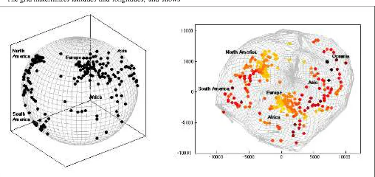
Data to be mapped are 273 large cities around the world. Their distances in the original space are calculated in the 3D space (Fig. 4-left). The mapping by DD-HDS is given in Fig. 4-right. It can be seen that the mapping accounts for the local density of cities. The north hemisphere is properly developed. Continents can be identified. Cities-free areas (like Pacific ocean, Antarctic, …) are distorted although continuity is preserved in most places.
The grid materializes latitudes and longitudes, and shows
the deformations resulting from the mapping. The grid was not used during the mapping process. It has been placed on the representation a posteriori, through interpolations between mapped cities: each intersection between latitude and longitude lines were placed in order to best fit its distances with cities in the original space (according to (8)). Points were then connected to give a lattice. This interpolation procedure is not specific to DD-HDS and could be used in a similar way with other mapping methods.
This example makes it possible to understand the viewpoint proposed by DD-HDS. Short distances are properly represented, while large ones are not necessarily mapped in a realistic way.
Fig. 4. Mapping of the earth globe (defined by large cities) in a 2D space. Color (right part) indicates the satisfaction of pairwise distances for the corresponding city (pressure, Eq. (10)). Darkest points indicate highest pressures. For clarity, the part of the grid close to the South Pole is not displayed.
B. Open boxes
Original data live in a 3D space. They are situated on the sides of two open cubes with open sides pointing toward two different directions (Fig. 5, upper left part). The mapping by DD-HDS is shown to its right. Under these plots, the Pi criterion (10) for each point (left), and the dy-dx
diagram (right) are shown. Others subplots display mappings achieved by competing methods.
This simulation illustrates on a simple example the advantages of DD-HDS. It correctly develops the two boxes, despite a twist on a large scale. The method effectively combines obvious nonlinear properties with a faithful representation of neighborhoods. Sammons' mapping gives a more expected view, but the lateral faces of the cubes are drastically compressed.
Even if nonlinear mappings are achieved with most methods, it can be seen that more or less intuitive representations are obtained. In the case of SOM, the two clusters are correctly found and neighborhoods are preserved, but the shape of the original objects is not recovered. Methods based on the geodesic concept (Isomap and LLE) give two disconnected plots for the two boxes as there is no path available between them (see § II B 2). The black line between the two box representations expresses this segmentation. The impact of long distances does not allow the development of the sides adjacent to the open side of the
boxes.
On the one hand, Sammon’s mapping does not generated any tear, but many false neighborhoods (just as PCA does). On the other hand, CCA succeed in mapping data without any false neighborhood, but some tears can be observed. This result was expected (see section III.B).
Except for the mapping produced by DD-HDS, all other show false neighborhoods and/or tears.
The two open boxes data set can be used to visualize the impact of λ (Fig. 6). High values for λ increase the quality of global structure representations (highest left panels) but neighborhood relations are jeopardized. Low values for λ (0.1 for example) permit a better neighborhood representation, but the overall shape is not guaranteed. Very low values for λ (here 0.05) generate “unreasonable” weighting functions although the mapping may be still found acceptable.
Fig. 5. Mapping of two 3D open boxes in a 2D space (The color codes for the position of the data in the original space (except for the local mapping efficiency and global mapping efficiency plots). Upper left set of subplots: upper left: original data (3D space), upper right: mapping by DD-HDS (2D space), lower left: pressure (Color lut is similar to Fig. 4), lower right, pairwise distance preservation (color codes for density of distances). Other subplots are self-explanatory. Isomap code used for this simulation is from http://isomap.stanford.edu/ , SOM is from Matlab Neural Network Toolbox (nnet), Sammon’s mapping and LLE are from http://www.cis.hut.fi/projects/somtoolbox/ .
Fig. 6. Mapping of the two boxes data set according to λ: left side; color code is the same as in Fig. 5; right side: associated distances in output space and corresponding weighting functions.
C. Face data
The set contains 698 pictures of the same virtual face under different angle and illumination conditions. It has been used by Tenenbaum [18] to test Isomap on high-dimensional data. The original dimension of the data is 4096 (number of pixels), and their intrinsic dimension should is 3 (two viewing angles and one illumination angle). Fig. 7 shows the mappings achieved by PCA, Sammon’s mapping, CCA and DD-HDS with Euclidean distance, and Isomap and DD-HDS with geodesic distance (five neighbors have been used to build the grid for geodesic distance). Each resulting map is displayed three times, from top to bottom in each column, but points are colored differently: from top to bottom, they are colored according to the horizontal viewing angle, the vertical viewing angle, and the illumination angle. Typical examples of images bordered by the color corresponding to the respective angle are shown in the left part of Fig. 7.
The intrinsic dimension of this data set is 3. Actually, most of the tested methods succeed in mapping these data onto a 3D space. However, maps on Fig. 7 are generated in a 2D space. This test cannot be perfectly passed: tears or false neighborhoods are unavoidable. Here, the challenge is to get as less tears as possible while avoiding false neighborhoods. As expected, PCA and Sammon’s mappings display high levels of false neighborhood and tears. DD-HDS and CCA with Euclidean distance effectively place points close from one another when their characteristics are similar. This can be seen through the fact that close points have similar colors on the three graphs. Nevertheless, much more exceptions (close points with different colors) are found with CCA. The methods illustrated in the two last columns of Fig. 7 (Isomap and DD-HD) use geodesic distance in the original space. It is much easier to observe
the continuity of the three intrinsic parameters (the three angles) in these two mappings. The horizontal angle is properly mapped by both methods. The vertical angle is also properly captured by Isomap, whereas DD-HDS provides a smooth mapping of light rotation. However, only DD-HDS mapping is such that almost all pairs of close points have similar values (colors) for each of the three angles. Having all three angles similar in a pair of points that are close in the mapping is indeed the necessary condition to have two close points corresponding to close faces (closes faces means that all three angles are similar). Although both Isomap and DD-HDS lead to close points that do not fulfill these requirements (again, tears and false neighbors are unavoidable in this application), Fig. 7 shows that the number of such situations is much lower in DD-HDS: a large number of false neighbors (in Isomap) has been replaced by a lower number of tears (in DD-HDS).
D. The genomic signature issues
Dealing with real data often rises problems that are not encountered with simulated data. In particular, the eventual complexity of real data distribution in high-dimensional space may strongly reduce mapping efficiency.
Genomic signatures are high-dimensional data resulting from the analysis of DNA sequences in terms of short oligonucleotide frequencies. Within the paradigm of genomic signature, DNA sequences are considered as “texts” build with a 4-letter alphabet (nucleotides A, T, C, G). Short oligonucleotides are small DNA sequences (usually 2 to 8 nucleotides long). It has been shown that the set of oligonucleotide frequencies calculated from a DNA sequence at least several thousands nucleotides long (the so-called genomic signature) is species specific i.e. different species have different signatures [24].
Similarities between species allow building a taxonomy of life, usually displayed as a tree (the famous tree of life).
Fig. 7. Representation of face data by PCA, Sammon’s mapping, CCA and DD-HDS (4 first columns, Euclidean distances) and Isomap and DD-HDS (2 last columns, geodesic distances). See text for details. Scales of distances are shown for the methods that respect Euclidean distances (Sammon’s mapping, CCA and DD-HDS on Euclidean distances).
Traditional taxonomy is essentially based on macroscopic observations about species. Genomic features may also be used. Along branches of the tree of life, successive refinements lead to an accurate description of species that are the leaves of the tree. For example, "root; cellular organims; Eukaryota; Fungi/Metazoa group; Metazoa; Eumetazoa; Bilateria; Coelomata; Deuterostomia; Chordata; Craniata; Vertebrata; Gnathostomata; Teleostomi; Euteleostomi; Sarcopterygii; Tetrapoda; Amniota; Mammalia; Theria; Eutheria; Euarchontoglires; Primates; Simiiformes; Catarrhini; Hominoidea; Hominidae; Homo/Pan/Gorilla group; Homo sapiens" is the path in the tree to a well k n o w n s p e c i e s ( N C B I : www .ncbi.nlm.nih.gov/Taxonomy/taxonomyhome.html ).
It has been shown that close species in terms of taxonomy have close signatures and vice versa. It is not realistic (yet?) to observe (and corroborate) the full tree of life using the genomic signature as a criterion. However, large partitions (at the bottom of the tree) as well as some specific branches are already properly described with it (see [64-66] for examples). It seems therefore interesting to check the ability of dimensionality reduction methods to preserve the taxonomic features of genomic signatures.
Depending on the size of examined oligonicleotides, the genomic signature may have a various number of dimensions, ranging usually from 16 to 65536. For this paper, we focused on 256-dimension signatures that have the most interesting properties with respect to taxonomy. The study presented here concerns 2046 genomic signatures illustrating the diversity of living organisms (697 Eukaryotes (plants, vertebrates, fungus, ...), 1349 Prokaryotes made up of 1287 bacteria and 62 archebacteria).
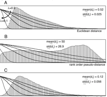
It has been shown that taxonomic information can be derived from genomic signatures by means of the Euclidean metric that allows characterizing similarity between them [25, 64]. Euclidean metric and derived “metrics” (rank and geodesic) were successively used within DD-HDS to
compare genomic signatures. According to the procedure described above, the weighting function was fitted to the various distributions of distances (Fig. 8). The interest of an adaptive weighting function is obvious here, considering the diversity in values and shapes of the distance distributions.
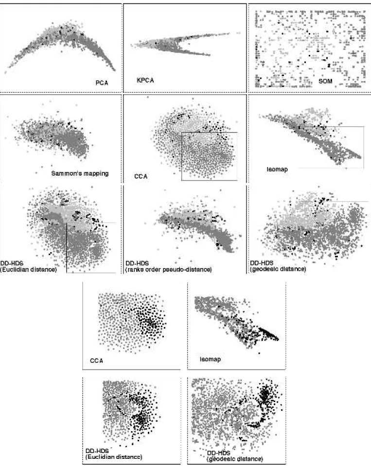
Fig. 9 shows the mapping obtained by PCA, KPCA, SOM, Sammon's mapping, CCA, Isomap, and DD-HDS using the three “metrics”. In the upper part of the figure, we are concerned with the ability of the mapping to express segmentation between signatures near the root of the tree of life. The groups the species belong to (namely Eukaryotes, bacteria and Archebacteria) are recognized by the gray intensity of points. Mappings achieved by PCA and KPCA do not clearly reveal the taxonomic features of the genomic signatures. The high non-linear correlations between variables are likely responsive for the typical croissant shaped layout. Although Sammon’s mapping makes a better use of the output space, it fails to display the species organization: the projection remains folded, because of the limitations resulting from the Sammon's stress weighting by distances in the original space, and also probably because of the concentration of measure phenomenon (see section III.B). Groups are not easily identifiable in the Kohonen map although a general organization of signatures is observable. Isomap allows separating Eukaryotes from bacteria but overlapping remains important. CCA offers an interesting display where groups can be localized and segmented. The paving-like structure may result from the ultimate preservation of short distances between signatures, considering that in high-dimensional Euclidean spaces, even “short” distances are “long”.
DD-HDS also offers mappings where groups of species can be segmented. In addition, DD-HDS provides a sharper separation between groups of species.
Mappings obtained using the rank order pseudo-distance and with ISOMAP are pretty close. The spatial orientation of data follows the nucleotide bias (frequencies of the nucleotides are not necessarily equal over species). It is already know in fact that although the nucleotide bias largely varies between species, it is not linked to taxonomy. The nucleotide bias explains an important part of the overall dispersion of genomic signatures in the high-dimensional space. It is also captured by PCA and KPCA. Mappings obtained from Euclidean distances and geodesic distances are more informative. In particular, substructures in data are observable (see subplots in Fig. 9, lower part, where actinobacteria are highlighted). They correspond to well-identified subgroups of species and are probably the expression of local substructures in the original space.
As bottom lines, we would like to point out that the mapping of genomic signatures achieved in this study would have been better, if more dimensions would have been allowed for the output space. Our experience with genomic signatures, DD-HDS and other experimental protocols suggests that the intrinsic dimension of the genomic signatures should be around 7-8.
rank order pseudo-distance std(d ) = 26.9i < j ij mean(d ) = 50i < j ij B geodesic distance (k=5) std(d ) = 0.056i < j ij mean(d ) = 0.12ij i < j C Euclidean distance std(d ) = 0.025ij i < j mean(d ) = 0.52ij i < j λ=0.1 λ=0.9 A
Fig. 8. Weighting functions fitted to the distributions of distances: A) Euclidean metric, B) rank order pseudo-metric and C) geodesic metric (connectivity=5).
Fig. 9. Mappings of 2046 genomic signatures. Upper panels: signatures as mapped by PCA, KPCA (polynomial kernel of degree 2), SOM (35X55 nodes), Sammon's mapping, Isomap (connectivity=5), CCA, and DD-HDS using Euclidean metric, and derived metrics or pseudo-metrics (rank order and geodesic (connectivity=5)); points correspond to species, grey levels code for taxonomy: light gray = Eukaryotes, dark gray = bacteria, black = archebacteria. Lower panels: Highlights of the subgroup of actinobacteria for some of the above mappings (others species are in grey).