HAL Id: hal-01494366
https://hal.archives-ouvertes.fr/hal-01494366
Submitted on 20 Mar 2020HAL is a multi-disciplinary open access archive for the deposit and dissemination of sci-entific research documents, whether they are pub-lished or not. The documents may come from teaching and research institutions in France or abroad, or from public or private research centers.
L’archive ouverte pluridisciplinaire HAL, est destinée au dépôt et à la diffusion de documents scientifiques de niveau recherche, publiés ou non, émanant des établissements d’enseignement et de recherche français ou étrangers, des laboratoires publics ou privés.
Bootstrapped artificial neural networks for the seismic
analysis of structural systems
Elisa Ferrario, Nicola Pedroni, Enrico Zio, Fernando Lopez-Caballero
To cite this version:
Elisa Ferrario, Nicola Pedroni, Enrico Zio, Fernando Lopez-Caballero. Bootstrapped artificial neural networks for the seismic analysis of structural systems. Structural Safety, Elsevier, 2017, 67 (1), pp.70-84. �10.1016/j.strusafe.2017.03.003�. �hal-01494366�
Bootstrapped Artificial Neural Networks for the seismic analysis of structural systems
E. Ferrario1, N. Pedroni2, E. Zio2,3 and F. Lopez-Caballero4
1Laboratory LGI, Université Paris-Saclay, Grande Voie des Vignes, 92290 Chatenay-Malabry, France 2Chair System Science and the Energy Challenge, Fondation Electricité de France (EDF), CentraleSupélec, Université
Paris-Saclay, Grande Voie des Vignes, 92290 Chatenay-Malabry, France 3Department of Energy, Politecnico di Milano, Italy
4Laboratory MSSMat, UMR CNRS 8579, CentraleSupélec, Université Paris-Saclay, Grande Voie des Vignes, 92290 Chatenay-Malabry, France
Abstract
We look at the behavior of structural systems under the occurrence of seismic events with the aim of identifying the fragility curves. Artificial Neural Network (ANN) empirical regression models are employed as fast-running surrogates of the (long-running) Finite Element Models (FEMs) that are typically adopted for the simulation of the system structural response. However, the use of regression models in safety critical applications raises concerns with regards to accuracy and precision. For this reason, we use the bootstrap method to quantify the uncertainty introduced by the ANN metamodel. An application is provided with respect to the evaluation of the structural damage (in this case, the maximal top displacement) of a masonry building subject to seismic risk. A family of structure fragility curves is identified, that accounts for both the (epistemic) uncertainty due to the use of ANN metamodels and the (epistemic) uncertainty due to the paucity of data available to infer the fragility parameters.
Keywords: seismic risk, structure, fragility curve, Artificial Neural Network, epistemic uncertainty, bootstrap, confidence intervals
Nomenclature
a : ground motion level
b : index of the bootstrap training data sets or of the bootstrapped regression models, b = 1, …, B B : number of the bootstrap training data sets or of the bootstrapped regression models
CP : coverage probability
D = {(Yn, n), n = 1, …, N} : entire data set
Dtrain = {(Yn, ( )), n = 1, …, Ntrain} : training data set
Dtrain,b : bootstrap training data set, b ∈ {1, …, B}
Dval = {(Yn, ( )), n = 1, …, Nval} : validation data set
Dtest = {(Yn, ( )), n = 1, …, Ntest} : test data set
E = network performance (energy function) f(Yn, w): regression function
fb(Yn, wb): bootstrapped regression function, b ∈ {1, …, B}
F : fragility curve
Fb : fragility curve built on the basis of the b-th bootstrapped regression function, b ∈ {1, …, B} : lower bound fragility curve due to the paucity of data
: upper bound fragility curve due to the paucity of data
: lower bound fragility curve due to the model and the paucity of data : upper bound fragility curve due to the model and the paucity of data
h : optimal number of hidden neurons
IArias : Arias intensity
j : index of the inputs Y L : likelihood function M : number of input variables n : index of the data in a given set
N : number of realization of the seismic event NMW : normalized mean width
Ntest : number of test data
Ntrain : number of training data
Nval : number of validation data
p : coverage indicator; p = 1 if the output is included in the confidence interval; p = 0 otherwise pgv : Peak Ground Velocity
PSA(Tstr) : spectral acceleration at the first-mode period of the structure
RMSEANN : root mean square error of the ANN trained with the whole training data set Dtrain
RMSEBoot : root mean square error of the bootstrap ensemble of ANNs
SI : spectral intensity Tm : mean period
Tp : predominant period
Tstr : fundamental period of the structure
w : vector of parameters of the regression functions
wb : vector of parameters of the b-th bootstrapped regression functions, b ∈ {1, …, B} X : outcome of a seismic event (Bernoulli random variable)
xn : realization of the Bernoulli random variable Xn
= {x1, x2, …, xn, …, xN} : vector of the realizations of the N Bernoulli random variable Xn, n = 1, …, N
y : ground motion IMs
Y = {y1, y2, …, yi, …, yM} : vector of M uncertain input variables Z = {z1, z2, …} : vector of system responses
Greek Letters
α : median ground motion intensity measure (IM)
: estimate of α
( )%, ( )% : 100(1 – θ)% confidence interval of α
β : logarithmic standard deviation
: estimate of β
( )%, ̅ ( )% : 100(1 – θ)% confidence interval of β 1 – γ : level of confidence for the bootstrap-based empirical PDFs
δ : target, maximal structural top displacement
( ) : model output (maximal structural top displacement) in correspondence of the n-th input vector Yn ANN(Yn) : estimate of the maximal structural top displacement obtained by the ANN
!"( ) : estimate of the maximal structural top displacement given by one of the b-th bootstrapped regression functions, b ∈ {1, …, B}
̅ !( ) : average of the B estimates !"( ), b = 1, …, B
FEM(Yn) : true maximal structural top displacement computed by the FEM
δ* : damage threshold
( &)%( ), ̅ ( &)%( ) : 100(1 – γ)% confidence interval of the quantity (Yn)
ε(Yn) : Gaussian white noise
1 – θ : level of confidence for parameters α and β '(( ) : nonlinear deterministic function
)* !( ) : bootstrap estimate of the variance of )+*( ,)
)+*( ) : variance of the distribution of the regression function f(Yn, w) )-*( ) : variance of ε(Yn)
Φ[∙] : standard Gaussian cumulative distribution
Acronyms
ANN : Artificial Neural Network CDF : Cumulative Distribution Function CP : Coverage Probability
GA : Genetic Algorithm IM : Intensity Measure LGP : Local Gaussian Process NMW : Normalized Mean Width NPP : Nuclear Power Plant PGA : Peak Ground Acceleration PDF : Probability Density Function RMSE : Root Mean Square Error RS : polynomial Response Surface SA : Spectral Acceleration
SPRA : Seismic Probabilistic Risk Assessment SVMs : Support Vector Machines
1. Introduction
In the aftermath of the Fukushima nuclear accident, the 5-year project SINAPS@ (Earthquake and Nuclear Facilities: Ensuring and Sustaining Safety) has been launched in France in 2013. One of the key objectives of the project is the quantitative assessment of the behavior of Nuclear Power Plants (NPPs) under the occurrence of a seismic event. In the framework of this project, we made a preliminary study on the behavior of a structural system subject to seismic risk [Ferrario et al., 2015], with the aim of identifying the structure fragility curve, i.e., the conditional probability of damage of a component for any given ground motion level [EPRI, 2003]. In this work, we complete the previous analysis with the estimation of the associated uncertainties.
Within the framework of analysis considered, in general the actions, events and physical phenomena that may cause damages to a nuclear (structural) system are described by complex mathematical models, which are then implemented into computer codes to simulate the behavior of the system of interest under various conditions [USNRC, 2009; NASA, 2010]. In particular, computer codes based on Finite Element Models (FEMs) are typically adopted for the simulation of the system structural behavior and response: an example is represented by the Gefdyn code [Aubry et al., 1986].
In practice, not all the system characteristics can be fully captured in the mathematical model. As a consequence, uncertainty is always present both in the values of the model input parameters and
variables and in the hypotheses supporting the model structure. This translates into variability in the
model outputs, whose uncertainty must be estimated for a realistic assessment of the (seismic) risk [Ellingwood and Kinali, 2009; Liel et al., 2009].
For the treatment of uncertainty in risk assessment, it is often convenient to distinguish two types: randomness due to inherent variability in the system behavior (aleatory uncertainty) and imprecision due to the lack of knowledge and information on the system (epistemic uncertainty). The former is related to random phenomena, like the occurrence of unexpected events (e.g., earthquakes) whereas the latter arises from a lack of knowledge of some phenomena and processes (e.g., the power level in the nuclear reactor), and/or from the paucity of operational and experimental data available [Apostolakis, 1990; Ferson and Ginzburg, 1996; USNRC, 2009; Aven, 2010; Aven and Zio, 2011 Beer et al., 2014].
For uncertainty characterization, two issues need to be considered: first, the assessment of the system behavior typically requires a very large number (e.g., several hundreds or thousands) of FEM simulations under many different scenarios and conditions, to fully explore the wide range of uncertainties affecting the system; second, FEMs are computationally expensive and may require
hours or even days to carry out a single simulation. This makes the computational burden associated with the analysis impracticable, at times.
In this context, fast-running regression models, also called metamodels (such as Artificial Neural Networks (ANNs) [Zio, 2006; Cardoso et al., 2008; Beer and Spanos, 2009; Pedroni et al., 2010; Chojaczyk et al., 2015], Local Gaussian Processes (LGPs) [Bichon et al., 2008; Villemonteix et al., 2009] polynomial Response Surfaces (RSs) [Bucher and Most, 2008; Liel et al., 2009], polynomial chaos expansions [Ciriello et al., 2013; Sudret and Mai, 2015], stochastic collocations [Babuska et al., 2010], Support Vector Machines (SVMs) [Hurtado, 2007] and kriging [Bect et al., 2012; Dubourg and Sudret, 2014; Zhang et al., 2015]), can be built by means of input-output data examples to approximate the response of the original long-running FEMs without requiring a detailed physical understanding and modeling of the system process, and used for the seismic analysis. Since the metamodel response is obtained quickly, the problem of high computational times is circumvented. However, the use of regression models in safety critical applications like NPPs still raises concerns as regards the control of their accuracy and precision.
In this work, we use ANN-based metamodels to approximate the response of a detailed FEM. To evaluate the approximation introduced by using the ANN metamodels in replacement of the detailed FEM, we can adopt three main approaches for the estimation of ANN accuracy and precision: the bootstrap method, based on a resampling technique [Efron, 1979; Efron and Tibshirani, 1993]; the delta method, based on a Taylor expansion of the regression function [Rivals and Personnaz, 1998; Dybowski and Roberts, 2001]; the Bayesian approach, based on Bayesian statistics [Bishop, 1995; Dybowski and Roberts, 2001]. We adopt the first one, because it requires no prior knowledge about the distribution function of the underlying population, being a distribution-free inference method [Efron and Thibshirani, 1993], it is simple to implement and provides accurate uncertainty estimates [Zio, 2006].
The effectiveness of ANN and bootstrap methods in robustly quantifying the uncertainty associated with (safety-related) estimates (possibly obtained with small-sized data sets) has been thoroughly demonstrated in the open literature: see, e.g., [Efron and Thibshirani, 1993; Zio, 2006; Pedroni et al., 2010; Zio and Pedroni, 2011].
In this work, we originally apply bootstrapped ANNs in seismic risk analysis for the estimation of fragility curves and the quantification of the corresponding uncertainty. For the analysis, we consider the same case study employed in [Ferrario et al., 2015], which consider the structural damages of a masonry structure subject to a seismic event [Lopez-Caballero et al., 2011]. First, we use the ANN metamodel to estimate the maximal structural top displacement, and its uncertainty in the form of
bootstrap-based confidence intervals. Then, we derive the corresponding family of fragility curves for a given damage threshold, taking into account both the variability of the maximal structural top displacement within the confidence intervals and the epistemic uncertainty due to paucity of data available for the estimation of the fragility curve parameters.
The paper organization is as follows. In Section 2, the steps necessary to build the fragility curves are illustrated and the sources of uncertainty identified; in Section 3, a synthetic description of ANN metamodels is provided; in Section 4, the uncertainty introduced by the ANN metamodels is described; in Section 5, the bootstrap approach for the estimation of the ANN uncertainty is given; in Section 6, the procedure for the bootstrapped ANN-based estimation of fragility curves in the presence of uncertainties is provided; in Section 7, the case study and the main results of the analysis are presented; in Section 8, conclusions and future developments are provided.
2. Analysis of the failure behavior of structural systems: fragility curve estimation
Within the framework of Seismic Probabilistic Risk Assessment (SPRA), a fragility curve, F, is the conditional probability of failure (i.e., of exceeding a level of damage) of a component/structure for any given ground motion level (i.e., peak ground acceleration – PGA – or peak spectral acceleration – SA – at different component or structural frequencies) [EPRI, 2003]. It represents in probabilistic terms the seismic capacity of a component/structure, in terms of the maximum ground motion level (PGA or SA) that a component/structure can sustain without failure. Both PGA and SA are good indicators of structural damage; however, most SPRAs are based on PGA since most existing hazard studies have focused primarily on it [EPRI, 2003].
It is standard practice to model the seismic capacity by a lognormal probability distribution and evaluate its parameters for critical failure modes by the Fragility Analysis [EPRI, 2003; Ulrich et al., 2014], though any measure of ground motion intensity can be used. The use of the lognormal distribution is justified by its mathematical simplicity and by the fact that it has been widely used for several decades in earthquake engineering: actually, it often fits the observed distributions of quantities of interest, such as ground motion intensity measures (IMs) [Porter, 2015].
In this paper, we retain the lognormal model assumption and we infer the associated parameters by the maximum likelihood method, taking into account the epistemic uncertainty in their estimates due to the paucity of data available.
In particular, we construct the fragility curve through the following three main steps: (a) structural system modeling;
(b) structural system behavior simulation; (c) fragility curve estimation.
In step (a), a mathematical model of the system is built to quantify its performance indicator. A quantitative model for seismic risk analysis may be viewed as composed of three main elements: a vector Y = {y1, y2, …, yj, …, yM} containing all the uncertain input variables (e.g., the ground motion IMs); a computer code to simulate the behavior of the system of interest; and an output vector Z = {z1, z2, …} describing the system responses (e.g., the maximal structural top displacement).
In step (b), the mathematical model is implemented in a computer code and used to simulate system behavior under different uncertain operational and accidental conditions: for N vectors Yn, n = 1, …,
N, of possible model input values (i.e., N seismic events in this case), N model outputs ( ), n = 1,
…, N, are computed. In order to deeply explore the wide range of uncertainties, a very large number (e.g., several thousands) of simulations is typically needed.
Finally, in step (c) the fragility curve F is estimated from the data (i.e., the N maximal structural top displacements ( ), n = 1, …, N) generated at step (b) above.
The mathematical formulation of the fragility is the following [EPRI, 2003]: = /( > ∗|3) = Φ
5678 9 :
;< , (1)
where is the maximal structural top displacement, * is the damage threshold, a is the ground motion level (e.g., PGA), Φ[∙] is the standard Gaussian cumulative distribution function (CDF), and
α and β are the parameters of the lognormal distribution of the seismic capacity, where α is the median
ground motion IM, i.e., the median ground acceleration capacity (e.g., median PGA), and β the logarithmic standard deviation.
Given the model outputs (Yn), n = 1, …, N, of step (b) above, the parameters α and β in equation (1) can be estimated through the maximum likelihood method [Shinozuka et al., 2000; Saez et al., 2011] by analyzing those outputs (Yn), n = 1, …, N, that exceed the damage threshold of interest *. The likelihood function L that has to be maximized to infer parameters α and β is:
=( ; , ) = ∏FG @ ABC@1 − A BC, (2)
where = {x1, x2, …, xn, …, xN} is the vector of the N realizations of a Bernoulli random variable X representing the outcome of a seismic event that can be classified into two mutually exclusive ways:
xn = 0, if the component/structure sustains the damage threshold * (i.e., (Yn) < *) for a given ground motion level a, and xn = 1, otherwise (i.e., (Yn) > *); Fn, n = 1, …, N, is the fragility value in correspondence of the n-th seismic event.
Two sources of uncertainty are involved in step (c), due to:
• aleatory uncertainty due to randomness in the structural seismic capacity, described by a lognormal distribution;
• epistemic uncertainty due to the finite amount of data available to infer the parameters (α and
β) of the lognormal distribution.
The seismic capacity is characterized by aleatory uncertainty: actually, the structural response results from randomness in the ground motion IM; thus, even with a large data set available, this uncertainty is irreducible. The classical way to address the uncertainty due to randomness is to collect data about the random phenomenon of interest (i.e., the ground motion) and perform a statistical analysis to identify the probability density function (PDF) that best captures the variability of the available data. The analyst’s choice of a particular shape of the PDF (i.e., lognormal) represents a source of epistemic uncertainty and can be progressively reduced by the analyst as the size of the available data set increases [Apostolakis, 1990]. In this work, we assume that the chosen lognormal PDF is a well-fitted model for the random seismic capacity (i.e., its shape acceptably represents the variability of the uncertain seismic capacity).
The (epistemic) uncertainty upon the distribution parameters (α and β) depends on the quantity of data available: the higher the number N of seismic events, the more accurate the estimates of the parameters. To account for this type of epistemic uncertainty, we consider the (1 – θ)% = 95%
confidence intervals (i.e., θ = 0.05) of the α and β estimates, i.e., ( )%, ( )% and ( )%, ̅ ( )% , respectively. Letting the parameters vary in their corresponding confidence intervals, a family of fragility curves is thereby obtained. Then, the upper and lower bounds, and , respectively, of these curves can be identified to provide a measure of the epistemic uncertainty associated with F due to the paucity of data.
A final remark is in order. Traditionally, computer codes based on FEMs are adopted for the simulation of structural systems behavior and response. Since FEMs are computationally expensive (e.g., they may require hours or even days to carry out a single simulation), the computational cost associated with the analysis may be prohibitive.
One possibility to overcome this computational issue is to resort to fast-running regression models (metamodels) to replace the detailed, long-running FEMs with acceptable approximation. In this work, we adopt ANNs (see Section 3) to reproduce the nonlinear relation between the vector Y of M inputs representing the different characteristics of the seismic event, like Peak Ground Velocity (pgv), Arias Intensity (IArias), Spectral Intensity (SI), etc., and one output, that is the maximal structural top
displacement , i.e., Z = {z1} = . The estimates provided by ANNs are affected by uncertainty (see Section 4) that can be quantified in terms of confidence intervals by the bootstrap approach (see Sections 5 and 6).
3. Artificial Neural Networks for nonlinear regression
Given a finite set of input/output data examples (patterns), D = {(Yn, (Yn)), n = 1, …, N} where Yn is a vector of input variables, Yn = {y1,n, y2,n, …, yj,n, …, yM,n}, and (Yn) is the output target (assumed mono-dimensional for simplicity of illustration), it is possible to perform the task of nonlinear regression, i.e., to estimate the nonlinear relationship between the vector of input variables and the output target.
It can be assumed that the target ( ), n ∈ {1, …, N}, is related to the input vector Yn by an unknown nonlinear deterministic function μ (Yn) corrupted by a Gaussian white noise ε(Yn) [Bishop, 1995], i.e,
( ) = '(( ) + I( ) ; I( ) ~ N(0, )-*( )) (3)
In the present case of damage of a structural system subject to seismic risk, the vector Yn, n ∈ {1, …,
N}, contains the ground motion IMs, the nonlinear deterministic function '(( ) is given by the
complex long-running FEM code, the variable ( ) represents the maximal structural top displacement and the noise ε(Yn) represents the error introduced by the numerical method employed to calculate μ (Yn).
The objective of the regression task by ANN is to estimate '(( ) through a regression function f(Yn,
w), that depends on the set of ANN parameters w. For the sake of clarity, in the rest of the paper we
will refer to JFF and to indicate the ANN and the FEM outputs, respectively.
ANNs are computing devices inspired by the function of the nerve cells in the brain [Bishop, 1995]. They are composed of many parallel computing units (called neurons or nodes) arranged in different layers and interconnected by weighed connections (called synapses). Each of these computing units performs few simple operations and communicates the results to its neighbouring units. From a mathematical viewpoint, ANNs consist of a set of nonlinear (e.g., sigmoidal) basis functions with adaptable parameters w that are adjusted by a training process on many different input/output data examples available in the data set Dtrain = {(Yn, (Yn)), n = 1, …, Ntrain}, where Dtrain is a subset of the entire data set D, as explained at the end of this Section. The training process is an iterative process of regression error minimization [Rumelhart et al., 1986]; it consists in optimizing the network performance E computed as, e.g., the average squared error between the network outputs
K =FLMNOC∑FGLMNOCQ JFF( ) − ( )R *
(4)
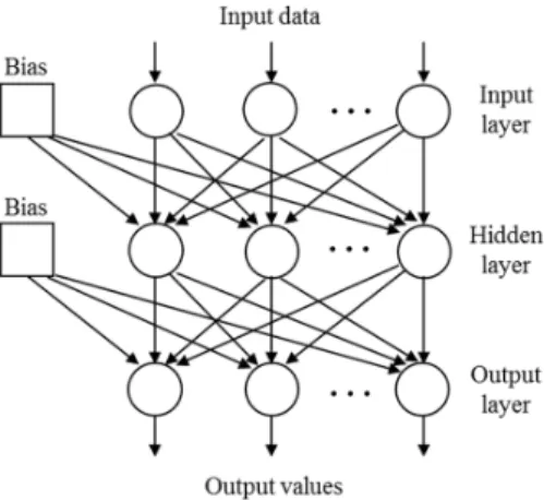
ANNs have been demonstrated to be universal approximants of continuous nonlinear functions (under mild mathematical conditions) [Cybenko, 1989], i.e., in principle, an ANN model with a properly selected architecture can be a consistent estimator of any continuous nonlinear function. The particular type of ANN considered in this paper is the classical feed-forward ANN composed of three layers (input, hidden and output, see Figure 1) and trained by the error back-propagation algorithm.
Figure 1. Scheme of a three-layered feed-forward Artificial Neural Network.
The number of nodes in the input layer equals the number of M input variables Yn = {y1,n, y2,n, …, yj,n, …, yM,n}, which significantly affect the output; the number of nodes in the output layer is determined by the number of quantities of interest to the problem (in this case one: the maximal structural top displacement, (Yn)); the number of nodes in the hidden layer in general is kept as low as possible, since the higher the number of hidden nodes, the higher the number of parameters (w) to be estimated and the stronger the requirements on the data needed for the estimation. In general, an ANN with too few hidden nodes does not succeed in learning the training data set; vice versa, an ANN with too many hidden nodes learns the training data set very well, but it does not have generalization capability.
Typically, the entire set of N input-output data is divided into three subsets:
• a training (input/output) data set (Dtrain = {(Yn, (Yn)), n = 1, …, Ntrain}), used to calibrate the adjustable parameters (w) of the ANN regression model, for best fitting the FEM data;
• a validation (input/output) data set (Dval = {(Yn, (Yn)), n = 1, …, Nval}, made of patterns different from those of the training set), used to monitor the accuracy of the ANN model during the training procedure. In practice, the validation error is computed on the validation set at different iterative stages of the training procedure: at the beginning of training, this value
decreases as does the error computed on the training set; later in the training, if the ANN regression model starts overfitting the data, the error calculated on the validation set starts increasing and the training process must be stopped [Bishop, 1995];
• a test (input/output) data set (Dtest = {(Yn, (Yn)), n = 1, …, Ntest}), not used during ANN training and validation, needed to evaluate the network generalization capability in the presence of new data.
Further details about ANN regression models are not reported here for brevity; the interested reader may refer to the cited references and the copious literature in the field.
4. Artificial Neural Network uncertainty
In regression models, there are two types of prediction that are computed in correspondence of a given input Yn, n ∈ {1, …, N}: 1) the model structure f(Yn, w), that is the estimate of the deterministic function μ (Yn), and 2) the model output (Yn) (eq. 3). In this work, we focus on the first one and associate to this estimate the corresponding measure of confidence.
In this respect, the uncertainty related to the identification of the parameters w has to be taken into account. This is mainly due to three reasons:
• The set Dtrain adopted to train the network cannot be exhaustive due to the limited number of input/output patterns that do not fill all the input volume of interest. As a consequence, different training sets Dtrain can give rise to different sets of network parameters w and, then, to different sets of regression functions, i.e., to a distribution of regression functions. The quantification of the accuracy of the estimate f(Yn, w) of the true deterministic function, μ (Yn), entails the assumption of a distribution for the regression error f(Yn, w) – μ (Yn). Its variance, E[f(Yn, w) – μ (Yn)]2, with respect to all possible training data set is given by the sum of two terms [Bishop, 1995; Zio, 2006]:
o the square of the bias, {E[f(Yn, w)] – μ (Yn)}2, that is the square of the difference between the expected value of the distribution of the regression functions, E[f(Y, w)], and the true deterministic function, μ (Yn);
o the variance, )+*( ), of the distribution of the regression functions:
)+*( ) = {f(Yn, w) – E[f(Yn, w)]}2 . (5)
Since the bias can be considered negligible with respect to the second term, the accuracy of the estimate f(Yn, w) is given by the variance )+*( ) of the distribution of the regression functions [Bishop, 1995; Zio, 2006]:
• The choice of the network architecture is inappropriate. If the number of hidden neurons is too small or too big, the network may not have the expected generalization capabilities (see Section 3). A trade-off can be achieved by controlling the number of parameters, and the training procedure, e.g., by early stopping of the training [Bishop, 1995; Zio, 2006].
• The global minimum of the error function (eq. 4) is not achieved: the minimization algorithm may get stuck in a local minimum and/or the training may be stopped before reaching the minimum [Bishop, 1995; Zio, 2006].
Thus, due to the uncertainties, for given model input parameters/variables Yn, n ∈ {1, …, N}, the model output (Yn) can vary within a range of possible values (e.g., confidence interval). For N vectors Yn, n = 1, …, N, of model inputs (i.e., N seismic events in this case), N model outputs ( ),
n = 1, …, N, can be computed with the associated N confidence intervals
( &)%( ), ̅ ( &)%( ) , n = 1, …, N, with (1 − U) level of confidence.
5. Bootstrap approach for ANN uncertainty estimation
To quantify the model uncertainty introduced by the ANN empirical regression models (see Section 4), the confidence intervals of the regression error f(Yn, w) – μ (Yn), where f(Yn, w) is the regression function given by the ANN and μ (Yn) is the deterministic function of the FEM, have to be estimated. One method is the bootstrap approach, that is capable of quantifying the model uncertainty by considering an ensemble of ANNs built on different data sets that are sampled with replacement (bootstrapped) from the original one [Zio, 2006]. From each bootstrap data set, a bootstrapped regression model is built and the model output of interest can be computed. Different bootstrap data sets give rise to a distribution of regression functions and so to a PDF of the model output. Thus, the model uncertainty of the estimates provided by the ANNs can be quantified in terms of confidence intervals of the obtained model output PDF by the bootstrap algorithm. An important advantage of this approach is that it provides confidence intervals for a given model output, without making any model assumption (e.g., normality). However, the computational cost could be high when the training data set and the number of parameters in the regression model are large [Pedroni et al., 2010].
The operative steps to identify the confidence intervals of the distribution of the regression error are detailed in the following:
1) Divide the entire available data set of N input/output patterns into training, validation and test data sets, as Dtrain = {(Yn, (Yn)), n = 1, …, Ntrain}, Dval = {(Yn, (Yn)), n = 1, …, Nval}
and Dtest = {(Yn, (Yn)), n = 1, …, Ntest}, respectively, where the outputs (Yn) are generated through the FEM code.
2) Generate B (e.g., B = 100 in this work) bootstrap training data sets, Dtrain,b, b = 1, …, B, by sampling with replacement from the original training data set Dtrain. Each set Dtrain,b, b ∈ {1, …, B}, is composed by the same number Ntrain of the original training data set; however, due to the sampling with replacement some of the input/output patterns in Dtrain will appear more than once in Dtrain,b, b ∈ {1, …, B}, whereas some will not appear at all.
3) Build the bootstrapped regression models fb(Yn, wb), b = 1, …, B, on the basis of the training data sets Dtrain,b, b = 1, …, B, generated at the previous step 2) and the validation data set Dval = {(Yn, FEM(Yn)), n = 1, …, Nval} of step 1) (Figure 2). The training data sets are used to calibrate the parameters wb, b = 1, …, B, and the validation data set to monitor the accuracy of the network performance (see Section 3).
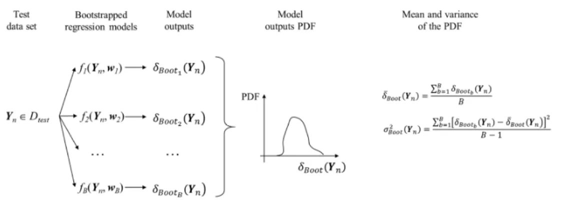
4) Use the regression models of step 3) to compute the estimates !"( ), b = 1, …, B, of the model output FEM(Yn) on a new data set Dtest = {(Yn, FEM(Yn)), n = 1, …, Ntest}. By so doing,
Ntest bootstrap-based empirical PDFs for the quantity FEM(Yn), n = 1, …, Ntest, are produced. In correspondence of a new input Yn, n ∈ {1, …, Ntest}, the bootstrap estimate ̅ !( ) is given by the average of the B regression functions !"( ), b = 1, …, B, n ∈ {1, …, Ntest}: ̅ !( ) = S( , VTW, X = 1, 2, … , [\) =∑"^_] +"( C,T")=∑]"^_(]``L"( C) (7)
and the bootstrap estimate )* !( ) of the variance )+*( ) in equation (5) is given by: )* !( ) =∑ (]``L"( C) (a]``L( C) b ] "^_ , n ∈ {1, …, Ntest} (8) as illustrated in Figure 3.
5) Identify the confidence intervals (with confidence level (1 − U)) from the bootstrap-based empirical PDF for the quantity FEM(Yn), n ∈ {1, …, Ntest}, obtained in step 4) as follows. For each test n ∈ {1, …, Ntest} compute the two-sided 100(1 – γ)% confidence intervals for the estimates !"( ), b = 1, …, B, by ordering the estimates !"( ), b = 1, …, B, in increasing values and identifying the (100γ/2)th and 100(1– γ/2)th quantiles of the bootstrap-based empirical PDF of the quantity FEM(Yn) as the closest values to the (Bγ/2)th and B(1 – γ/2)th elements, respectively. In the following, the confidence interval of FEM(Yn), n ∈ {1, …, Ntest}, are referred to as ( &)%( ), ̅ ( &)%( ) .
To determine the quality of the confidence intervals identified in step 5), two quantitative measures can be taken into account [Ak et al., 2013]: the coverage probability (CP) and the normalized mean
width (NMW). The former represents the probability that the true values FEM(Yn), n = 1, …, Ntest, are included in the corresponding confidence intervals, whereas the latter quantify the extension of the confidence intervals and it is usually normalized with respect to the minimum and maximum values of FEM(Yn), n = {1, …, Ntrain}. They are conflicting measures since the wider NMW the larger CP, and in practice it is important to have large coverage and small width.
The CP is given by [Ak et al., 2013]: c/ =FLdeL∑FLdeLf
G , (9)
where f = 1 if FEM(Yn) ∈ ( &)%( ), ̅ ( &)%( ) ; otherwise f = 0, for n = 1, …,
Ntest.
The NMW is computed as [Ak et al., 2013]:
hij =F LdeL∑ (a_kk(_lm)%( C) (_kk(_lm)%( C) (nNo (nOC FLdeL G (10)
where max and min are the maximum and minimum values of the FEM outputs, respectively.
The estimates given by the bootstrapped ANNs, ̅ !( ), are in general more accurate than the estimate of the best ANN, JFF( ), in the bootstrap ensemble of ANNs (that is the one trained with the original data set, Dtrain, as shown in step 1) above) [Zio, 2006; Zio and Pedroni, 2011]. Actually, the ANNs ensemble has diverse (higher) generalization capabilities than the best ANN. This can be verified through the estimation of the Root Mean Square Error (RMSE) for the bootstrap ensemble of ANNs (RMSEBoot) and the best ANN (RMSEANN) with respect to the true output ( ) of the FEM, as follows:
piqK ! = rFLdeL∑FLdeLG Q ̅ !( ) − ( )R* (11)
Figure 2: Exemplification of step 3 of the bootstrap method of Section 5: construction of the bootstrapped regression models given the training and validation data sets.
Figure 3: Exemplification of step 4 of the bootstrap method of Section 5: construction of the bootstrap-based empirical PDF of the model output for a new input Yn of the test data set.
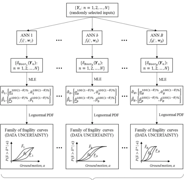
6. Bootstrapped ANN-based estimation of fragility curves in the presence of uncertainties The complete procedure is as follows (Figure 4):
1) given an ensemble of B properly trained ANNs VS( |sW): X = 1, 2, … , [\, for N randomly generated vectors , n = 1, 2, …, N, of model inputs (i.e., N seismic events), evaluate the corresponding model outputs !"( ), b = 1, 2, …, B, n = 1, 2, …, N (see Section 5); 2) for each ANN b = 1, 2, …, B, of the ensemble, evaluate the parameters W and W of the
fragility curves and the corresponding CIs, [ W ( )%( ), W ( )%( )A and [ W ( )%( ), ̅W ( )%( )A, respectively, by MLE (see Section 2);
3) for each ANN of the ensemble, letting parameters α and β range within the corresponding CIs
[ W ( )%( ), W ( )%( )A and [ W ( )%( ), ̅W ( )%( )A (step 2 above), generate a family of fragility curves (under the lognormal assumption) and identify the corresponding upper and lower bounds, W and W, respectively;
4) identify the extreme upper and lower fragility curves, and , respectively, that envelop all the bootstrapped fragility curves V( W, W): X = 1, 2, … , [\ thereby obtained.
The curves produced at step 4) represent bounds that describe and take into account the epistemic uncertainty due to
1) the data for the extrapolation of the distribution parameters α and β of the seismic capacity (step (c) of Section 2) and
2) the model (the ANN) for the estimation of the model output (step (b) of Section 2).
Notice that in this case the runs of the (bootstrapped) ANNs are only needed to generate a set of model outputs !"( ), b = 1, 2, …, B, n = 1, 2, …, N, for each bootstrapped ANN. Then, on the basis of these new sets of data (produced by each ANN b of the ensemble), the parameters W and W of the fragility curves and the associated CIs, [ W ( )%( ), W ( )%( )A and [ W ( )%( ), ̅W ( )%( )A, can be estimated by MLE. Notice that for each given ANN b =
1, 2, …, B, of the bootstrap, the CIs [ W ( )%( ), W ( )%( )A and
[ W ( )%( ), ̅W ( )%( )A mentioned above reflect the (epistemic) uncertainty related to the scarcity of the data available for the extrapolation of the distribution parameters W and W. Moreover, it is worth stressing again that the need to resort to ANNs (and in general to metamodels) derives from the very high computational cost required by each FEM run (i.e., several hours), which would impair further, more thorough uncertainty and sensitivity analyses on the system model of interest, if needed. Also, the additional advantage of adopting bootstrapped ANNs instead of a single
ANN is represented by the possibility of computing CIs ( &)%( ), ̅ ( &)%( ) for the model outputs, in order to take into account also the epistemic (model) uncertainty associated with the use of ANN regression functions trained with a finite-sized set of data (see Section 5).
A final remark is in order with respect to step (2) of the algorithm above. The fact that here we adopt a parametric approach, i.e., we assume a lognormal probability distribution for the fragility curve and use the MLE method for the estimation of the corresponding parameters, does not absolutely impair the effectiveness and general applicability of our bootstrapped ANN-based approach. Actually, once the metamodels are properly trained and validated, (i) they enable detailed uncertainty and sensitivity
analyses of computationally expensive FEMs for structural risk assessment (if required); and (ii) they could be used to build the fragility curves of interest according to any other method available in the open literature (e.g., non-parametric approaches relying on repeated Monte Carlo-based pointwise estimations of the conditional failure probability for many different values of the selected earthquake intensity measure).
Figure 4: Exemplification of the procedure for the bootstrapped ANN-based estimation of fragility curves in presence of uncertainty.
7. Case study
The case study is taken from [Lopez-Caballero et al., 2011]. It deals with the non-linear soil influence on the seismic response of a two-story masonry structure founded on a rigid shallow foundation. In Section 7.1, the description of the specific system studied is given; in Section 7.2, the results of the uncertainty analysis are provided, together with some critical considerations.
7.1. Case study description
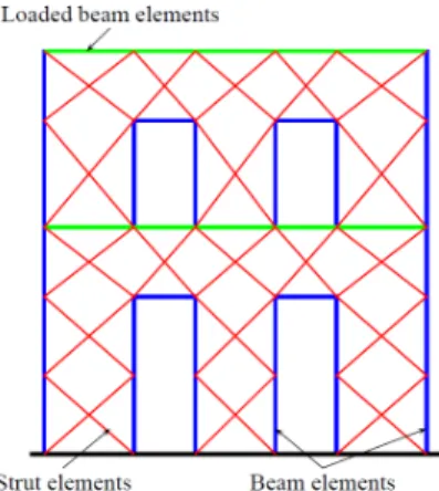
The masonry building analyzed in this work is illustrated in Figure 5. The total height of the building is 5.4 m, the width is 5.0 m and the thickness is 0.16 m. With these characteristics, the fundamental period of the structure (Tstr) is equal to 0.19 s. This structure is modelled using three different kinds of elements: beam-columns and diagonal struts describing the structural behavior, and strengthless solid elements to represent the masonry mass. The frame structural elements are modelled by plastic hinge beam-column elements. The behavior of this structure is simulated on the basis of non-linear dynamic FE analysis. Further details about the masonry characteristics and the FEM used are not reported here for brevity sake; the interested reader is referred to [Lopez-Caballero et al., 2011].
Figure 5: Building scheme.
In order to define appropriate ground motions for the non-linear dynamical analysis, a selection of N = 168 recorded accelerograms from the Pacific Earthquake Engineering Research Center (PEER) database have been used as input to the model. The events range between 5.2 and 7.6 in magnitude and the recordings have site-to-source distances from 15 to 50 km, and dense-to-firm conditions (i.e., 360 m/s < Vs30 < 800 m/s, where Vs30 is the average shear wave velocity in the upper 30 m).
The information carried by each single earthquake signal has been synthetized by thirteen IM parameters [Lopez-Caballero et al., 2011]. In this work, we take into account just the five IM parameters reported in Table 1 that have been selected by the authors in [Ferrario et al., 2015] by performing a Genetic Algorithm (GA)-based wrapper feature selection aimed at identifying the subset
of important inputs that maximize the ANN performance. These selected parameters form the input vector Yn = {y1,n, y2,n, …, yM = 5,n}, n ∈ {1, …, N = 168}.
Table 1: IM earthquake parameters (model inputs: Y = y1, y2, …, yM = 5).
Y
y1 IArias Arias intensity
y2 PSA(Tstr) Spectral acceleration at the first-mode period of the structure
y3 Tm Mean period
y4 Tp Predominant period
y5 SI Spectral intensity
In the following, we refer to the model inputs by their numbers (i.e., y1, y2, y3 …) instead of their name (IArias, PSA(Tstr), Tm, …) for brevity.
7.2. Results
ANNs are used in order to approximate the nonlinear seismic response of the masonry building of interest. A data set composed by N = 168 input/output patterns is available for the analysis. In order to train, validate and test the ANN, the N data are partitioned as follows: 70% in the training set (i.e.,
Ntrain = 118 data), 15% in the validation set (i.e., Nval = 25 data) and 15% in the test set (i.e., Ntest = 25 data).
In Section 7.2.1, the results of the estimation of the accuracy of the ANN by the bootstrap approach (Section 5) is reported; then, in Section 7.2.2 the computation of the structure fragility curves under uncertainty (Section 6) is illustrated.
7.2.1. ANN accuracy
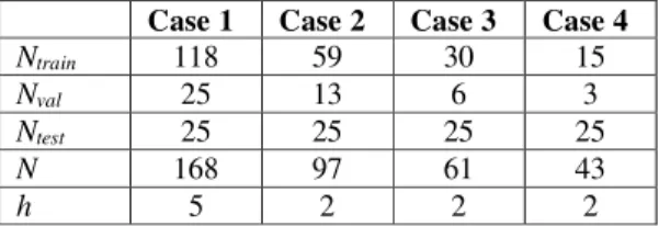
To estimate the ANN accuracy, the bootstrap approach of Section 5 has been applied. The analysis has been performed with respect to four different sizes of the training and validation sets, to evaluate the network accuracy in cases where smaller data sets are available. Indeed, the seismic fragility analysis and the estimation of confidence bounds based on recorded ground motions is usually performed with a number of analyses that is smaller than or comparable to 168 (for critical infrastructures), also due to limitations in the number of suitable recorded ground motions available. In Table 2, the total number N of input/output data adopted, and the number of those used in the training (Ntrain), validation (Nval) and test (Ntest) are reported, with respect to the four cases analyzed. Case 1 considers all the N = 168 data available, so it is composed by the largest training and validation sets (Ntrain = 118, Nval = 25); cases 2, 3 and 4 halve the training and validation sets of their previous case, e.g., the training and validation sets of case 2 are the rounded half of those of case 1 (i.e., Ntrain = 59, Nval = 13). The size of the test data set is kept constant for all the four cases (Ntest = 25 data), in order to perform a comparison of the network accuracy. All the networks have been trained with a
number h of hidden nodes optimized with respect to the training and validation procedures for each network (Table 2).
Table 2: Number of patterns in the training (Ntrain), validation (Nval), and test (Ntest) data sets for the four different cases
evaluated; N is the total number of data and h is the optimal number of hidden neurons adopted to train and validate a single network.
Case 1 Case 2 Case 3 Case 4
Ntrain 118 59 30 15
Nval 25 13 6 3
Ntest 25 25 25 25
N 168 97 61 43
h 5 2 2 2
As a first general analysis to evaluate the accuracy of the regression estimate of '(( ), we have computed the following performance indicator that represents the average standard deviation ) !
ua
on the mean value:
) !ua =FLdeL∑ rv]``L
b ( C)
FLdeL
G , (13)
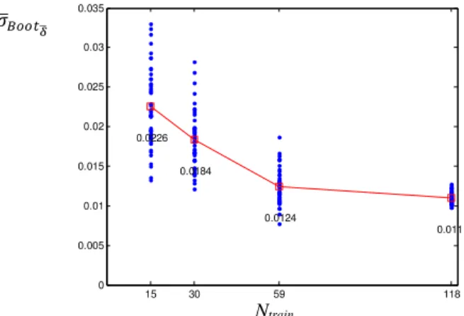
where )* !( ) is the bootstrap variance given in equation (8) and B is the number of bootstrapped networks considered (B = 100 in this study). The results are reported in Figure 6 with respect to the test data set, i.e., Yn = 1, …, Ntest, for the four cases of interest of Table 2, where Ntrain takes values equal to 118, 59, 30 and 15 data. For each case, several (i.e., 50) simulations (represented by the dots in the Figure) are run in order to account for the variability associated with the (randomly sampled) initial training and validation data sets, and to the random sampling with replacement implied by the bootstrap. Notice that in the reference case where Ntrain = 118, the training and validation data sets are the same for all the 50 simulations (since they correspond to the whole training data set); then, the variability in these results is due only to the bootstrap sampling. It can be seen that the lower the size of the training and validation data sets, the lower the network accuracy: the average of the ) !
ua
values (depicted by the squares in the Figure) increases from 0.0111 in case 1 (Ntrain = 118) to 0.0233 in case 4 (Ntrain = 15).
Figure 6: Dots: ) !ua computed on the test data set with respect to different sizes of the training data set (Ntrain).
Squares: average of ) !ua for a given size of the training data set.
Some of the ) !
ua values in Figure 6 are far from their average. From the analysis of the
corresponding box plot (Figure 7), these points (represented by a plus sign) are outliers since they are outside the box and the whiskers (in this case, the edges of the box represent the 25th and 75th percentiles and those of the whiskers the 99.3 coverage, if the data are normally distributed). The presence of outliers can be explained by the fact that some of the bootstrapped networks may not be well trained because of: (i) “unlucky” configurations of the initial training and validation data sets due to random sampling with replacement implied by the bootstrap (for example, a too large number of repeated samples may be contained in the design of experiments), or (ii) inefficient calibration of the ANN weights during training (for example, the back-propagation algorithm may get stuck in a local optimum). In this case, some biased network components of the bootstrap ensemble may not be able to estimate the model output with a satisfactory level of accuracy and may significantly degrade the estimate of the average of the bootstrapped regression functions ̅ !, thus providing an overestimate of the variance )* !. As suggested in [Zio, 2006], a possible way to tackle this issue is to actually train a large number of bootstrap networks and then retain only those which are regarded as well trained. In this light, for illustration purposes, we remove the outliers from Figure 6 and we compute again the average of the remaining ) !
ua values (squares in Figure 8) with the sole aim of
highlighting the general “trend” of the ANN accuracy with respect to the size of available training data set. It can be seen that without outliers it is more evident that the smaller the size of the training data set, the larger the value of the average of ) !
ua, so the smaller the network accuracy.
For completeness, the average standard deviation values σaxyyz
{a computed on the training data set
(i.e., by replacing Ntest with Ntrain in equation (13)) is reported in Figure 9. The same considerations can be drawn on the average trend: the smaller the training data set, the higher the standard deviation.
15 30 59 118 0 0.01 0.02 0.03 0.04 0.05 0.06 0.07 0.08 0.0111 0.0142 0.0216 0.0233 ) !ua Ntrain
Figure 7: Box plot of ) !ua computed on the test data set with respect to different sizes of the training data set (Ntrain).
Figure 8: Dots: ) !ua computed on the test data set with respect to different sizes of the training data set (Ntrain).
Squares: average of ) !
ua for a given size of the training data set. The outliers highlighted in Figure 6 have been
removed.
Figure 9: Dots: ) !
ua computed on the training data set with respect to different sizes of the training data set, (Ntrain).
Squares: average of ) !
ua for a given size of the training data set.
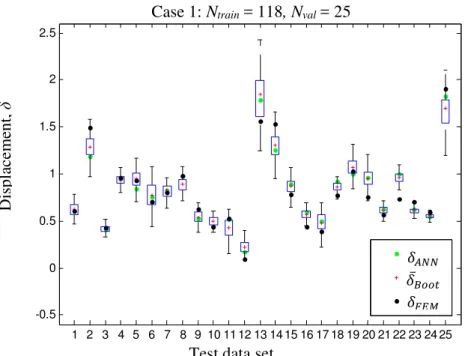
The 50% confidence intervals | %( ), ̅| %( ) for the quantity FEM(Yn) on the test data set,
n = 1, …, Ntest = 25, obtained by the bootstrap approach (Section 5) are illustrated by the box plots of 15 30 59 118 0 0.01 0.02 0.03 0.04 0.05 0.06 0.07 0.08 15 30 59 118 0 0.005 0.01 0.015 0.02 0.025 0.03 0.035 0.011 0.0124 0.0184 0.0226 15 30 59 118 0 0.005 0.01 0.015 0.02 0.025 0.03 0.035 0.0049 0.0058 0.0079 0.0109 ) !ua Ntrain Ntrain ) !ua Ntrain ) !ua
Figures 10 – 13, with respect to the four cases of Table 2, where the edges of the box represent the 25th and 75th percentiles and those of the whiskers the 99.3 coverage if the data are normally distributed. The estimates of the best ANN, ANN, (light dots) and of the bootstrap ensemble of ANNs,
̅ ! (plus signs), are reported together with the true output, FEM (dark dots).
Figure 10: Confidence intervals of the quantity FEM(Yn) (dark dots) given by the bootstrap approach with respect to the
test data set for the case 1 of Table 2. The estimates of the best ANN, ANN, (light dots) and of the bootstrap ensemble of ANNs, ̅ !, (plus signs) are also reported.
-0.5 0 0.5 1 1.5 2 2.5 1 2 3 4 5 6 7 8 9 10 11 12 13 14 15 16 17 18 19 20 21 22 23 24 25 δANN δBoot δFEM JFF ̅ !
Case 1: Ntrain = 118, Nval = 25
Test data set
D is pl ac e m ent , δ
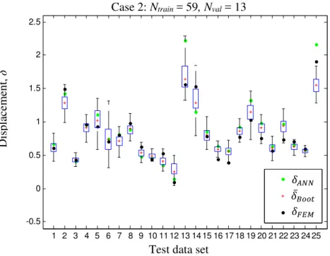
Figure 11: Confidence intervals of the quantity FEM(Yn) (dark dots) given by the bootstrap approach with respect to the
test data set for the case 2 of Table 2. The estimates of the best ANN, ANN, (light dots) and of the bootstrap ensemble of ANNs, ̅ !, (plus signs) are also reported.
Figure 12: Confidence intervals of the quantity FEM(Yn) (dark dots) given by the bootstrap approach with respect to the
test data set for the case 3 of Table 2. The estimates of the best ANN, ANN, (light dots) and of the bootstrap ensemble of ANNs, ̅ !, (plus signs) are also reported.
-0.5 0 0.5 1 1.5 2 2.5 1 2 3 4 5 6 7 8 9 10 11 12 13 14 15 16 17 18 19 20 21 22 23 24 25 δANN δBoot δFEM -0.5 0 0.5 1 1.5 2 2.5 1 2 3 4 5 6 7 8 9 10 11 12 13 14 15 16 17 18 19 20 21 22 23 24 25 δANN δBoot δFEM
Case 2: Ntrain = 59, Nval = 13
Test data set
D is pl ac e m ent , δ
Test data set
D is pl ac em e nt , δ
Case 3: Ntrain = 30, Nval = 6
JFF
̅ !
JFF
Figure 13: Confidence intervals of the quantity FEM(Yn) (dark dots) given by the bootstrap approach with respect to the
test data set for the case 4 of Table 2. The estimates of the best ANN, ANN, (light dots) and of the bootstrap ensemble of ANNs, ̅ !, (plus signs) are also reported.
In Table 3, the rankings of the standard deviation values ) !( ), n = 1, …, Ntest, computed from equation (8) for the model outputs !"( ), b = 1, …, 100, n = 1, …, Ntest, are reported with respect to the different amount of data available for the training and validation processes. In general, the smaller the number of input/output patterns used to train (and validate) the network, the larger the probability to find standard deviation values, ) !( ), n = 1, …, Ntest, higher than a given threshold. For example, with respect to a threshold equal to 0.1, this probability is equal to 13/25 ~ 0.5 in case 1 and doubles up to 25/25 = 1 in case 4.
From Table 3 it can be seen also that the highest values of ) !( ) (at the top of the ranking) are registered in correspondence of the inputs Yn, n = 6, 13, 14, 25, for all the four cases considered. Thus, the outputs associated with these inputs are affected by high uncertainty. This can be explained by looking to Figure 14, where the Ntest input/output test patterns (circle) are illustrated together with the
N input/output data (dots) with respect to IM y1 (IArias). The regression model may not fit well the test points 6, 13, 14 and 25 since they are at the border of the data cloud and, in addition, they are (except for test point 6) at the top of the Figure characterized by a plastic force-displacement behavior that is more difficult to predict.
-0.5 0 0.5 1 1.5 2 2.5 1 2 3 4 5 6 7 8 9 10 11 12 13 14 15 16 17 18 19 20 21 22 23 24 25 δANN δBoot δFEM
Test data set
D is pl ac e m ent , δ
Case 4: Ntrain = 15, Nval = 3
JFF
Table 3: Bootstrap standard deviation estimates ) !( ) , n = 1, …, Ntest = 25, of the model outputs !", b = 1, …,
100.
Figure 14: Input/output patterns with respect to the logarithm of the intensity measure y1 (IArias).
To estimate the quality of the 50% confidence intervals, | %( ), ̅| %( ) , for the quantity FEM(Yn) shown in Figures 10 – 13, the CP (CP) with respect to the output given by the FEM and the
n σBoo t n σBoo t n σBoo t n σBo ot
13 0.40 13 0.55 13 0.43 13 0.46 25 0.29 14 0.47 14 0.32 14 0.41 6 0.19 6 0.22 25 0.24 6 0.34 14 0.19 12 0.22 6 0.22 12 0.31 17 0.15 5 0.18 2 0.18 25 0.31 2 0.15 19 0.15 5 0.18 2 0.30 7 0.14 15 0.13 19 0.17 22 0.26 11 0.12 25 0.13 12 0.16 7 0.24 5 0.12 8 0.13 15 0.15 18 0.24 19 0.11 2 0.12 8 0.15 5 0.23 15 0.11 7 0.12 20 0.15 19 0.22 20 0.11 22 0.12 22 0.14 4 0.19 9 0.10 20 0.12 11 0.14 15 0.19 8 0.09 11 0.11 4 0.14 20 0.17 12 0.08 4 0.10 18 0.14 21 0.16 1 0.08 17 0.09 7 0.13 1 0.15 22 0.07 18 0.08 21 0.11 17 0.14 18 0.06 1 0.08 1 0.10 8 0.13 16 0.06 21 0.07 17 0.09 11 0.12 10 0.06 9 0.07 3 0.08 23 0.12 4 0.06 16 0.06 9 0.07 10 0.11 21 0.05 3 0.05 10 0.07 24 0.11 3 0.04 23 0.05 16 0.06 3 0.11 23 0.03 10 0.05 23 0.06 16 0.10 24 0.03 24 0.04 24 0.06 9 0.10
Case 1 Case 2 Case 3 Case 4
-5 -4 -3 -2 -1 0 1 2 0 0.2 0.4 0.6 0.8 1 1.2 1.4 1.6 1.8 2 1 2 3 4 5 6 7 8 9 10 11 12 13 14 15 16 17 18 19 20 21 22 23 24 25
log(y1) = log(IArias)
D is pl ac em ent , δ
NMW (NMW) (eqs. 9 and 10, respectively) are illustrated in Figure 15 for the four cases under analysis. Notice that to compare the estimates of the NMW, the normalization has been performed with respect to the max and min values of the test data set, i.e., in equation 10, }:B = max( ( )) and }• = min( ( )), n = 1, …, Ntest, that is the same for all the cases analyzed.
As expected, the smaller the number of data used to train and validate the network, the higher both the CP and the NMW of the intervals. The complement to 1 of CP has been plotted on the horizontal axis to highlight the conflict between these two measures (that are in fact on a Pareto frontier). Actually, an estimate is considered satisfactory if the corresponding confidence interval is characterized by high coverage and small width.
Case 1 Case 2 Case 3 Case 4
Ntrain 118 59 30 15
Nval 25 13 6 3
CP 0.280 0.320 0.480 0.600
NMW 0.067 0.080 0.094 0.123
Figure 15: Coverage probability (CP) with respect to the true output given by the FEM and Normalized Mean Width (NMW).
A comparison between the estimates given by the bootstrap ensemble of ANNs and the best ANN computed is given by the computation of the RMSEs, i.e., by RMSEBoot (eq. 11) and RMSEANN (eq. 12), respectively, as reported in Table 4 for the four cases of interest. As expected, the smaller the training data set, the higher the RMSEs. In addition, RMSEBoot is always lower than RMSEANN. This confirms the findings reported in the literature with respect to the superior estimation accuracy of the
0 0.1 0.2 0.3 0.4 0.5 0.6 0.7 0.8 0.9 1 0 0.02 0.04 0.06 0.08 0.1 0.12 0.14 0.16 0.18 0.2 Case 1 Case 2 Case 3 Case 4 1 – CP NMW
bootstrap aggregation procedure. In particular, the smaller the training data set, the higher the accuracy of the bootstrap ensemble compared to that of the best ANN: the percentage difference between the RMSEBoot and RMSEANN is around 5% for case 1 and 38% for case 4.
Table 4: Percentage of the Root Mean Square Errors (RMSEs) of the best ANN (RMSEANN) and of the bootstrap
ensemble of ANNs (RMSEBoot) with respect to the true output given by the FEM.
Case 1 Case 2 Case 3 Case 4
Ntrain 118 59 30 15
Nval 25 13 6 3
RMSEANN (%) 13.6 20.7 33.6 26.4
RMSEBoot (%) 12.9 13.7 20.5 16.4
7.2.2. Fragility curves
As recalled in Section 2, the fragility curve is the probability of exceeding a damage threshold of interest, *, for a given ground motion level. For illustration purposes, we assume a damage threshold
* equal to 0.63 cm (that corresponds to a slight damage of the structure) and we build the fragility
curve on the test data set, where Ntest = 25. The following evaluations are carried out with respect to an ANN trained with Ntrain = 118 data (case 1 of Table 2).
The α and β parameters estimated by the maximum likelihood method with respect to the ANN output (i.e., the displacement ANN) assume values equal to 1.02 and 1.17, respectively. The corresponding
estimates of the 95% confidence intervals are „|%, „|% = [0.32, 1.73] and „|%, ̅„|% = [0.88, 1.96], respectively. In Figure 16, the fragility curve F (solid line) is illustrated together with its lower, (dotted line), and upper, (dashed line), bounds: these bounds represent the epistemic uncertainty on the estimates of the α and β parameters due to the paucity of data (Ntest = 25); actually, such bounds are intended to envelop all the fragility curves that can be generated by all the possible combinations of α and β values ranging in their corresponding CIs. It can be noticed a discontinuity when the fragility is equal to 0.5. This is due to the properties of the lognormal distributions: the CDFs characterized by the same value of α and different values of β intersect in 0.5. In Figure 17, the intersections of the CDFs obtained by combining the highest and lowest values of the confidence intervals of α and β are illustrated. It can be seen that the upper bound is given by α equal to the minimum value ( = „|%) and β equal to the maximum value ( = ̅„|%) if the fragility is lower than 0.5, and to the minimum value ( = „|%) otherwise; vice versa, the lower bound is identified by α equal to the maximum value ( = „|%) and β equal to the minimum value ( = „|%) if the fragility is lower than 0.5, and to the maximum value ( = ̅„|%) otherwise.
Figure 16: Estimated fragility curve F (solid line) with the corresponding upper, (dashed line), and lower, F (dotted line), bounds representing the epistemic uncertainty due to the data.
Figure 17: Intersections of the fragility curves in correspondence of the combinations of the highest and lowest values of the parameters α and β.
In order to include also the model uncertainty due to ANN regression, the bootstrap approach of Section 5 is carried out. For each bootstrapped regression models b, the outputs !"( ), b ∈ {1, …, B}, n = 1, …, Ntest, are computed. Then, a fragility curve F and its lower F and upper bounds are estimated, as illustrated in Sections 2 and 6. Repeating this procedure for all the B bootstrapped regression models, a family of fragility curves Fb, b = 1, …, B, is obtained (Figure 18, left) and the corresponding families of the lower Fb and upper W bounds, b = 1, …, B, are determined (Figure 18, right). These results are combined in Figure 19 where the solid lines envelope all the possible fragility curves Fb, b = 1, …, B, and represent the epistemic uncertainty due to the ANN model; the dotted and
dashed lines represent the extreme lower ( ) and upper ( ) bounds of all the fragility curves, and they account both for the uncertainties due to the ANN model and to the data.
0 0.5 1 1.5 2 2.5 3 3.5 4 4.5 5 0 0.1 0.2 0.3 0.4 0.5 0.6 0.7 0.8 0.9 1 damage > 0.63 upper bound lower bound 0 1 2 3 4 5 0 0.1 0.2 0.3 0.4 0.5 0.6 0.7 0.8 0.9 1 ( „|%, ̅„|%) ( „|%, „|%) ( „|%, „|%) ( „|%, ̅„|%) F F
Ground motion level
C o n d it io n a l p ro b ab il it y o f ex c ee d in g a d a m a g e th re sh o ld
Ground motion level
C o n d it io n a l p ro b ab il it y o f ex c ee d in g a d a m a g e t h re sh o ld
Figure 18: Left: fragility curves Fb, b = 1, …, B, estimated from the B bootstrapped networks; right: corresponding
upper, W, (dashed lines) and lower , Fb,(dotted lined) bounds of the fragility curves, b = 1, …, B.
Figure 19: Uncertainty due to the network and the data of the fragility curves. Solid lines: upper and lower bounds of the fragility curves Fb, b = 1, …, B, estimated from the B bootstrapped networks (network uncertainty). Dashed and
dotted lines: corresponding upper and lower bounds, , and ,respectively (network and data uncertainty).
8. Conclusions
In the context of seismic risk analysis, FEMs are typically employed to simulate the structural response of a system; however, the computational burden associated with this analysis is impracticable, at times. This is due to the presence of large (aleatory and epistemic) uncertainties affecting the system. As a consequence, to explore their wide range of variability, a very large number (e.g., several thousands) of FEM simulations is required for an accurate assessment of the system behavior under different seismic conditions. In addition, long calculations (hours of even days) are necessary for each run of the FEM.
For these reasons, in [Ferrario et al., 2015] the authors have explored the possibility of replacing the FEM by a fast-running regression model, i.e., the ANN, to reduce the computational costs. The results showed a satisfactory capability of ANNs to approximating the FEM output in less than a second.
0 1 2 3 4 5 0 0.1 0.2 0.3 0.4 0.5 0.6 0.7 0.8 0.9 1 Fragility 0 0.5 1 1.5 2 2.5 3 3.5 4 4.5 5 0 0.1 0.2 0.3 0.4 0.5 0.6 0.7 0.8 0.9 1 upper bound lower bound 0 1 2 3 4 5 0 0.1 0.2 0.3 0.4 0.5 0.6 0.7 0.8 0.9 1 fragility upper bound lower bound Fb Fb W F C o n d it io n a l p ro b ab il it y o f ex c ee d in g a d a m a g e th re sh o ld C o n d it io n a l p ro b ab il it y o f ex c ee d in g a d a m a g e th re sh o ld C o n d it io n a l p ro b ab il it y o f ex c ee d in g a d a m a g e th re sh o ld
Ground motion level Ground motion level