HAL Id: hal-00297195
https://hal.archives-ouvertes.fr/hal-00297195
Submitted on 15 Nov 2006
HAL is a multi-disciplinary open access
archive for the deposit and dissemination of
sci-entific research documents, whether they are
pub-lished or not. The documents may come from
teaching and research institutions in France or
abroad, or from public or private research centers.
L’archive ouverte pluridisciplinaire HAL, est
destinée au dépôt et à la diffusion de documents
scientifiques de niveau recherche, publiés ou non,
émanant des établissements d’enseignement et de
recherche français ou étrangers, des laboratoires
publics ou privés.
The total ozone field separated into meteorological
regimes ? Part II: Northern Hemisphere mid-latitude
total ozone trends
R. D. Hudson, M. F. Andrade, M. B. Follette, A. D. Frolov
To cite this version:
R. D. Hudson, M. F. Andrade, M. B. Follette, A. D. Frolov. The total ozone field separated into
meteorological regimes ? Part II: Northern Hemisphere mid-latitude total ozone trends. Atmospheric
Chemistry and Physics, European Geosciences Union, 2006, 6 (12), pp.5183-5191. �hal-00297195�
www.atmos-chem-phys.net/6/5183/2006/ © Author(s) 2006. This work is licensed under a Creative Commons License.
Chemistry
and Physics
The total ozone field separated into meteorological regimes –
Part II: Northern Hemisphere mid-latitude total ozone trends
R. D. Hudson1, M. F. Andrade2, M. B. Follette1, and A. D. Frolov3
1Department of Atmospheric and Oceanic Science, University of Maryland, College Park, MD 20742-2425, USA 2Atmospheric Physics Laboratory, Campus Universitario Cota-Cota, Calle 27, Universidad Mayor de San Andres, La Paz,
Bolivia
3STG, Inc., 11710 Plaza America Drive, Reston, VA, USA
Received: 7 June 2006 – Published in Atmos. Chem. Phys. Discuss.: 11 July 2006 Revised: 13 October 2006 – Accepted: 8 November 2006 – Published: 15 November 2006
Abstract. Previous studies have presented clear evidence that the Northern Hemisphere total ozone field can be sep-arated into distinct regimes (tropical, midlatitude, polar, and arctic) the boundaries of which are associated with the sub-tropical and polar upper troposphere fronts, and in the winter, the polar vortex. This paper presents a study of total ozone variability within these regimes, from 1979–2003, using data from the TOMS instruments. The change in ozone within each regime for the period January 1979–May 1991, a pe-riod of rapid total ozone change, was studied in detail. Pre-vious studies had observed a zonal linear trend of −3.15% per decade for the latitude band 25◦–60◦N. When the ozone field is separated by regime, linear trends of −1.4%, 2.3%, and 3.0%, per decade for the tropical, midlatitude, and polar regimes, respectively, are observed. The changes in the rel-ative areas of the regimes were also derived from the ozone data. The relative area of the polar regime decreased by about 20%; the tropical regime increased by about 10% over this period. No significant change was detected for the midlat-itude regime. From the trends in the relative area and total ozone it is deduced that 35% of the trend between 25◦ and 60◦N, from January 1979–May 1991 is due to movement of the upper troposphere fronts. The changes in the relative areas can be associated with a change in the mean latitude of the subtropical and polar fronts within the latitude inter-val 25◦to 60◦N. Over the period from January 1979 to May 1991, both fronts moved northward by 1.1±0.2 degrees per decade. Over the entire period of the study, 1979–2003, the subtropical front moved northward at a rate of 1.1±0.1 de-grees per decade, while the polar front moved by 0.5±0.1 degrees per decade.
Correspondence to:R. D. Hudson ([email protected])
1 Introduction
In a previous paper, Hudson et al. (2003), presented clear evidence that the Northern Hemisphere total ozone field can be separated into distinct regimes, the boundaries of which are associated with the subtropical and polar upper tropo-sphere fronts, and in the winter, the polar vortex. These regimes were defined as: (1) the arctic regime – within the polar vortex, (2) the polar regime – between the polar front and the polar vortex, or when the latter is not present, the pole, (3) the midlatitude regime – between the subtropical and polar fronts, and (4) the tropical regime – between the equator and the subtropical front. The subtropical and po-lar fronts are associated with the subtropical and popo-lar jet streams, and have mean latitudes of about 30◦and 60◦N, re-spectively. It should be noted that the mean position of the subtropical front as defined here, is not the same as the posi-tion of the maximum of the mean westerly tropospheric zonal winds, which is also sometimes referred to as the subtropi-cal front (Bluestein, 1993). The positions of the subtropisubtropi-cal and polar fronts defined in Hudson et al. (2003) vary on a daily basis as the Rossby waves meander about their mean latitudes. Finally, these fronts should not be confused with the cold and warm fronts associated with cyclonic flow close to the surface. Hudson et al. (2003) showed, using rawin-sonde measurements, that the tropical, midlatitude, and polar regimes were identified with distinct tropopause heights over a large latitude range. In addition, in any month, a unique total ozone value and a distinct ozone profile shape could be assigned to each of these three regimes.
The definition of “mid-latitude” used in previous studies has varied. WMO (1999) and Staehelin et al. (2001) used the interval from 25◦ to 60◦N, while Fioletov et al. (2002) and WMO (2003) used the interval from 35◦ to 60◦N. In this paper we have chosen the latitude range from 25◦ to 60◦N. Previous studies of the variability of total ozone and of
5184 R. D. Hudson et al.: Total ozone trends within meteorological regimes the ozone profiles at midlatitudes (Harris et al., 1997, 1998;
WMO, 1999; Staehelin et al., 2001) have centered on zonal averages over specific latitude bands. However, because the mean total ozone and the ozone profile are almost constant within a regime, a zonal average will depend on the relative areas of the respective regimes within the latitude range of the zone. Thus, for example, one can envision a long-term change in the zonal mean total ozone that is brought about by a long-term change in the relative areas of the regimes alone.
The total ozone archived data sets used in this paper are the Version 8 level-3 hierarchical data format product from the TOMS (Total Ozone Mapping Spectrometer) instruments (McPeters et al., 1996; Wellemeyer et al., 2004). The level-3 data set is an average ozone value on a 1-degree lati-tude by 1.25 degrees longilati-tude grid. At this time three data sets are available, those from the Nimbus-7 satellite (November 1978–May 1993), the Meteor-3 satellite (Au-gust 1992–November 1994), and the Earth Probe satellite, (September 1996–December 2003), leaving a gap in the data record between December 1994 and August 1996. Although the 7 and Meteor-3 time periods overlap, Nimbus-7 data was used whenever available. The unit used within this paper for the total (column) ozone is the Dobson Unit (1 DU=1 m atm cm, or 2.69×10¹⁶molecules cm−2).
This paper examines the long-term change of ozone be-tween 1979 and 2003 within the tropical, midlatitude, polar, and arctic meteorological regimes as defined above. It is di-vided into four sections. In Sect. 2, the method used to define the boundaries between the regimes is presented. The results of the analysis are given in Sect. 3. The summary and con-clusions of the paper are given in Sect. 4.
2 The regime boundaries
For every day that TOMS data was available, total ozone val-ues for the subtropical and polar boundaries were derived us-ing the method described in Hudson et al. (2003). A contour program for these two boundary values was then used to ob-tain the positions of the fronts on the total ozone field for that day. The polar vortex boundary was obtained from the position of the maximum gradient in potential vorticity (PV) on the 550 K isentropic surface. This dataset was obtained from the NCEP/NCAR (National Centers for Environmen-tal Prediction/National Center for Atmospheric Research) re-analysis (Kalnay et al., 1996). Figure 1a shows the TOMS total ozone field for 11 March 1990, with the ozone contours representing the subtropical and polar boundaries, and the arctic boundary obtained from the PV field for this day. Fig-ure 1b shows the one-degree zonally averaged total ozone within each regime, and for the unclassified data. As noted in Hudson et al. (2003) and seen in Fig. 1b, each regime has a distinct range of ozone values that do not overlap. How-ever, the total ozone within each regime shows that there is
a small dependence (relative to the unclassified data) of to-tal ozone with latitude. This latitude dependence is greatest in the winter months, and is at a minimum in the summer months. Because trends in total ozone are of the order of few percent, small errors in the determination on the location of the upplevel fronts could introduce relatively large er-rors in the determination of long term area trends. For that reason, the latitude dependence of total ozone must be taken into account when determining the location of the upper-level fronts for trend analysis. It should be stressed, however, that the total ozone trends within each regime are not sensitive to small errors in the determination of the exact locations of the upper-level fronts.
A new method was developed in order to allow the bound-aries to take into account any latitude dependence. The daily boundary values from Hudson et al. (2003) were used as a first guess to separate the total ozone into regimes. Next, one-degree zonal averages were calculated for each regime, as seen in Fig. 1b. New subtropical boundary values were com-puted by taking the average of the tropical and midlatitude total ozone at each latitude where they were both present. Similarly, the polar boundary was calculated by taking the average of the midlatitude and polar total ozone. The new boundary values are displayed as black stars on Fig. 1b. The total ozone field was then separated using these new latitudi-nally dependent boundaries. The process was then repeated with the new boundary values. The relative area of a regime is the area of a regime divided by the total area between 25◦ and 60◦N. Convergence was reached when the change in the relative area of each regime, from one iteration to the next, was less than 5%. The 5% convergence criteria was chosen based on the spatial resolution of the TOMS data, 1◦
lati-tude by 1.25◦longitude. In each iteration, any change in the
area of a particular regime will have a minimum value given by the area of one pixel at each one-degree latitude band, which varies from 2–4%. The final boundaries, after itera-tion, are plotted on Fig. 1c. It must be stressed that these ozone boundaries were obtained on a daily basis.
Using the daily values, the mean monthly relative area was obtained for each regime, for the latitude interval 25◦–60◦N. The standard deviation, persistence, and the standard error of the mean were then calculated for each month. Table 1 gives the climatalogical mean monthly relative area, the standard error of the mean, and the atmopsheric persistence in days for the tropical, midlatitude, and polar regimes, for the pe-riod 1979–2003. The atmospheric persistence is defined here as (1+q)/(1−q) where q is the lag-1 autocorrelation. The at-mospheric persistence is close to three days, typical of mete-orological parameters.
A fundamental assumption in our method is that total ozone acts as a dynamical tracer on synoptic timescales (Danielsen et al., 1970; Wohltmann, 2005). This assumption is valid in the absence of chemistry occurring on timescales shorter than dynamics. Therefore, because our boundaries are calculated on a daily basis, they are subject to changes
Fig. 1. (a) TOMS total ozone field for 11 March 1990. The subtropical (blue line), polar (red line), and polar vortex (black line) boundaries derived by Hudson et al. (2003) are also plotted. (b) The one-degree zonally averaged total ozone within the tropical (red stars), midlatitude (green stars), polar (blue stars), and arctic (light blue stars) regimes for 11 March 1990. The unclassified data is shown as black pluses. The new boundary values calculated by taking the average of neighboring regimes are shown as black stars. (c) Same as (a), except with the boundaries after the iteration procedure described in the text.
in ozone chemistry on timescales shorter than a day. How-ever, in the lower stratosphere, the photochemical lifetime of ozone is of the order of several weeks (Brasseur and Solomon, 1984). This is large compared to the timescale of transport, approximately one day (Salby and Callaghan, 1993). For this reason, ozone in this region, as well as total ozone, is considered to be a dynamical tracer on the timescale of a few days (Wohltmann et al., 2005).
An experiment was carried out to test whether a latitudi-nally dependent chemical trend in ozone over time would affect the placement of the regime boundaries. Two runs from NASA Goddard Space Flight Center’s (GSFC) 3-D Full Chemistry and Transport Model (FCTM, Douglass et al., 1996) were used. The transport in this model is calculated off-line, such that the chemical constituents have no influ-ence over the model dynamics. The resolution of the model
was 4◦longitude by 5◦latitude, with 28 levels in the
verti-cal. Both heterogeneous, as well as gas-phase chemistry are included. The wind fields were derived using data from the NASA GSFC Data Assimilation Office (DAO). The first run was from February 1973 to December 2022, with observed aerosol and source gas concentrations The second run was from January 1979 to December 2010, and was the same as the first, except source gases were held to their 1979 value. The actual time period used for this experiment was 1983– 2003. The constant source gas run required several years of spin-up time (A. Douglass, personal communication), and corresponding time periods were desired. The positions of the meteorological upper-troposphere fronts should be the same in both runs. The ozone boundaries were then calcu-lated for both runs using the method described above, and the relative areas calculated from 1983–2003. There was no
5186 R. D. Hudson et al.: Total ozone trends within meteorological regimes
Table 1. Mean relative area, error of the mean, and persistence.
Tropical Regime Midlatitude Regime Polar Regime
Month Mean Error of Persistence Mean Error of Persistence Mean Error of Persistence area the mean (Days) area the mean (Days) area the mean (Days)
Jan 0.39 0.02 2.8 0.43 0.02 3.8 0.16 0.01 4.5 Feb 0.37 0.02 3.4 0.43 0.02 3.9 0.17 0.01 3.4 March 0.35 0.02 3.0 0.45 0.02 3.8 0.18 0.02 4.6 April 0.32 0.02 3.4 0.48 0.02 4.1 0.19 0.01 4.0 May 0.28 0.02 3.5 0.51 0.02 4.0 0.21 0.01 3.4 June 0.32 0.02 4.1 0.50 0.02 4.4 0.18 0.01 3.4 July 0.34 0.02 3.1 0.52 0.02 3.6 0.14 0.01 3.8 Aug 0.35 0.02 3.3 0.55 0.02 3.2 0.11 0.01 2.5 Sep 0.40 0.02 3.4 0.49 0.02 3.6 0.11 0.01 2.6 Oct 0.42 0.02 2.5 0.44 0.02 2.9 0.11 0.01 2.7 Nov 0.43 0.02 2.9 0.42 0.02 3.1 0.12 0.01 3.4 Dec 0.39 0.02 2.8 0.43 0.02 3.0 0.14 0.01 4.5
Fig. 2. Monthly mean total ozone values for the (a) zonal data, (b) tropical regime, (c) midlatitude regime, (d) polar regime, and (e) arctic regime for 25◦–60◦N, 1979–2003. Note the different scales.
statistically significant difference in the relative areas of each regime between the two runs, and no significant relative area trends were identified. It is concluded that long-term changes in ozone do not introduce a bias in the relative area trends.
3 Results
In the following analysis two different monthly means for the regimes are presented. First, all of the data between 25◦and 60◦N are used, corresponding to the zonal average between 25◦and 60◦N. If a pixel contains a boundary, its total ozone
value and area are halved and assigned to the two regimes separated by the boundary. This data set will be labeled as the “zero degree” data set. Next, the regions within one pixel in both latitude and longitude of the boundaries have been excluded from the analysis. This data set will be labeled as the “one degree” data set.
Figure 2 presents the area-weighted monthly mean total ozone values obtained from the TOMS data set, for the period 1979–2003 over the latitude range 25◦–60◦N. The monthly means shown in Fig. 2 are derived from the zero degree data set. Figure 2a shows the monthly mean total ozone values
Fig. 3. Same as Fig. 2, except the monthly climatology calculated from 1979 to 2003 has been removed. Note the different scales.
Table 2. Mean total ozone values and trends for zero-degree data set.
Regime Mean (DU) Trend per decade (DU)a Trend per decade (percent)a
Tropical 286 −3.9±1.4 −1.4±1.0
Midlatitude 331 −7.6±1.6 −2.3±0.5
Polar 394 −11.9±3.1 −3.0±0.7
Arctic 215 −5.2±9.0 −1.5±1.2
Zonal 326 −10.2±2.0 −3.1±0.7
aAll trends calculated from January 1979 to May 1991. All errors are two-sigma.
obtained without separation into the regimes (hereinafter re-ferred to as the “zonal data”), while Figs. 2b–e show data for the tropical, midlatitude, polar, and arctic regimes, respec-tively. As expected, the monthly mean total ozone values have a strong seasonal dependence. In addition, the arctic regime is not seen below 60◦N from about May to October. In Figs. 3a–e we have plotted the data shown in Fig. 2 after the seasonal component has been removed. This deseason-alization was done by subtracting the monthly mean clima-tology for the 1979–2003 period. It should be noted that not all of the fluctuations seen in the deseasonalized zonal data can be found in the corresponding data for each regime. The two strong downward fluctuations seen in the zonal data in 1985 and 1988 can be seen in the tropical regime, but not in the midlatitude or polar regime. Similarly the downward fluctuation seen in 1997 is only found in the polar regime.
Linear trends and their respective errors for the zonal and regime total ozone were obtained using the statistical time
se-ries model described in Stolarski et al. (2006). The time pe-riod from January 1979 to May 1991 was chosen because it is a period when the chlorine loading in the stratosphere varied almost linearly with time. The mean values for each regime and the zonal data, in addition to their trends and trend er-rors for the zero degree data set can be found in Table 2. All errors shown in this paper are two-sigma (95% confidence interval). Similar results for the one degree data set can be found in Table 3. Within the experimental error there is no difference between the trends shown in the two tables. The trend in DU per decade for the zonal total ozone corresponds to a percentage trend of −3.1±0.7 per decade, in excellent agreement with previous estimates (WMO, 1999; Staehelin et al., 2001).
Let the areas of the tropical, midlatitude, polar, and arctic regimes between 25◦ and 60◦N be AT, AM, AP, and AA,
respectively. The corresponding mean area-weighted total ozone values are defined as T, M, P, and A. Noting
5188 R. D. Hudson et al.: Total ozone trends within meteorological regimes
Table 3. Mean total ozone values and trends for one-degree data set.
Regime Mean (DU) Trend per decade (DU)a Trend per decade (percent)a
Tropical 280 −3.7±2.4 −1.3±1.0
Midlatitude 333 −7.2±1.6 −2.2±0.6
Polar 407 −11.8±3.5 −2.9±0.9
Arctic 191 −6.3±9.4 −3.2±3.8
aAll trends calculated from January 1979 to May 1991. All errors are two-sigma.
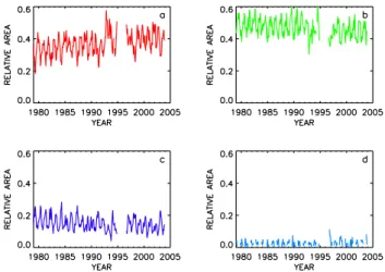
Fig. 4. Monthly mean relative areas of the (a) tropical regime, (b) midlatitude regime, (c) polar regime, and (d) arctic regime for 25◦– 60◦N, 1979–2003.
that is the column ozone per unit area, equivalent to col-umn mass per unit area, the total mass of ozone between 25◦ and 60◦N, M, can be written as:
M = cAo=cATT +cAMM+cAPP +cAAA(1)
In this equation, A is the total area between 25◦and 60◦N, O is the mean of the zonal data, and c is a constant of
pro-portionality. Dividing both sides of the equation by cA we get
o=RTT +RMM +RPP +RAA (2)
Here, the Rs are defined as the relative areas of the regimes. We can now examine the importance of each term on the right-hand side of Eq. (2) to the calculation of zonal total ozone.
The monthly mean relative areas derived from the TOMS data for the tropical, midlatitude, polar, and arctic regimes, between 25◦and 60◦N, for the period 1979–2003, are shown in Figs. 4a–d, respectively. The zero degree data set was used for all relative area analyses. The relative area for the trop-ical regime shows a clear increase between 1979 and 1992, and appears to level off after 1996. The relative areas of the polar and midlatitude regimes show a clear decrease between
Fig. 5. Same as Fig. 4, except the monthly climatology calculated from 1979 to 2003 has been removed.
1979 and 1992, followed also by a leveling off. The results for the arctic show almost no trend, however data for this regime is only available in the winter months. Figures 5a–d show the same data after the monthly climatology calculated between 1979 and 2003 has been removed. The mean val-ues, trends, and trend errors for each regime can be found in Table 4 and were calculated in the same manner as for the total ozone. The regimes in which a large change in the relative area is observed are the polar and tropical regimes. Between January 1979 and May 1991, the relative area of the polar regime decreased by about 20%, while that of the tropi-cal regime increased by about 10%. There was no significant change in the relative area of the midlatitude regime over this time period. These changes imply a net poleward movement of the subtropical and polar upper-troposphere fronts.
Figure 6 presents the contribution (in DU) of each term on the right hand side of Eq. (2). It should be noted that the contribution is positive for the tropical regime. This re-flects the fact that the area of the tropical regime is expand-ing at a faster rate than the rate of decay of its mean total ozone. The contribution of the arctic regime over this period is only 0.1 DU and shows little change with time. From Jan-uary 1979 to May 1991, the polar and midlatitude regimes show net losses of 16.7, and 10.0 DU, respectively. The trop-ical and arctic regimes show a net gain of 11.8, and 0.1,
Fig. 6. Monthly mean mass contribution (in DU) by the (a) tropi-cal regime, (b) midlatitude regime, (c) polar regime, and (d) arctic regime for 25◦–60◦N, 1979–2003.
Table 4. Mean relative areas and trends.
Regime Mean Trend per decade (×10−2)a Tropical 0.35 2.9±1.3
Midlatitude 0.48 −0.4±1.0 Polar 0.16 −2.6±1.1 Arctic 0.02 −0.0±0.5
aAll trends calculated from January 1979 to May 1991. All errors are two-sigma.
respectively. The sum of these changes is a loss of 14.8 DU, which agrees well with the loss in the zonal ozone data of 14.9 DU over the same time period.
4 Summary and conclusions
A major conclusion of this paper is that the downward trend in total ozone of 3.1% per decade over the period January 1979 to May 1991, for the mid-latitude zone from 25◦– 60◦N, is due to a combination of (1) a net reduction of total ozone for each of the three regimes defined by Hudson et al. (2003), and (2) a change in the relative weighting among the regimes due to a net movement of the polar and subtrop-ical fronts northward. Previous interpretations (Staehelin et al., 2001; Solomon et al., 1996, 1998) have concluded that this zonal total ozone trend was the result of increased ho-mogeneous and heterogeneous chemistry in the stratosphere. However, other studies have argued that long-term dynam-ical changes could be partly or largely responsible for the ozone trend (Fusco and Salby, 1999; Graf et al., 1998). Hood et al. (1999) estimated that up to 40% of the observed mid-latitude trend could be due to changes in stratospheric dy-namics. In a later paper, Hood and Soukharev (2005) con-cluded that nonlocal EP flux variations and local PV
vari-Table 5. Terms in Eq. (3).
Regime dA/dta A d/dta Tropical 8.4 −1.3 Midlatitude −1.3 −3.6 Polar −10.6 −1.7 Arctic −1.2 −0.1 Total −3.6 −7.0
aAll trends calculated from January 1979 to May 1991.
ations contributed at least 50% to observed negative trends in February near 40◦–50◦N. Statistical analyses have also shown that the Northern Hemisphere ozone trends are highly correlated with modes of variability of the atmospheric cir-culation, such as the Arctic Oscillation (AO), accounting for about 70–80% of the long-term ozone decline (Krzyscin et al., 2001). Reinsel et al. (2005) found the AO/AAO and EP flux index series had a considerable influence on total ozone at latitudes poleward of 40◦N. Hadjinicolaou et al. (2005)
examined dynamically-driven trends in total ozone using a three dimensional chemical transport model, the transport being derived from the European Centre for Medium-Range Weather Forecasts analysis. The conclusion of their paper is that over the period 1979 to 1993, the dynamically driven model trend accounted for 30% of the observed Northern Hemisphere negative trend, and all of the 1994–2003 positive trend. Salby and Callaghan (2002) found that most (80%) of the changes in total ozone during the 1980s and 1990s were coherent with anomalous forcing of the upward Eliassen-Palm flux from the troposphere and the quasi-biennial oscil-lation. The remaining 20% was almost entirely accounted for by including aerosol and chlorine forcing. Koch et al. (2002) conclude that in the lower stratosphere, dynamical transport processes dominate the day-to-day as well as the interannual variability of mid-latitude ozone.
Equation (2) can be differentiated with respect to time to yield: d dt = dT dt RT + dRT dt T + dM dt RM + dRM dt M +dP dt RP + dRP dt P + dA dt RA+ dRA dt A (3) The variation of total ozone with time for each regime is represented by two terms, one in which the total ozone is fixed and the area changes, and the other in which the area remains constant but the total ozone value changes. The re-sults for each of the terms shown in Eq. (3) are given in Ta-ble 5. The mean values and slopes used to calculate each term in Eq. (3) can be found in Tables 2 and 4. The sum of the terms when the area remains constant is −7.0 DU and the sum when the total ozone remains constant is −3.6 DU. Thus from this analysis, we would conclude that about 35% of the observed total ozone trend between January 1979 and May
5190 R. D. Hudson et al.: Total ozone trends within meteorological regimes 1991 is due to the northward movement of the fronts. The
remaining 65% is due to changes within each regime. These changes can be the result of chemical processes and/or dy-namical mechanisms, such as a net strengthening or weaken-ing of the Brewer-Dobson circulation (Randel et al., 2002). The analysis was also repeated for the period from 1996 to 2003, however, the errors in the constants became much larger, and no significant conclusion could be drawn for this time period.
The relative areas discussed above can be used to calculate the mean latitude of the subtropical and polar fronts for the latitude range from 25◦to 60◦N. A linear fit of the resulting mean latitudes from 1979 to 2003 yields a mean latitude shift northward of about one degree per decade for the subtropi-cal front, and 0.5 degrees per decade for the polar front. It should be noted that significant portions of the polar regime, and therefore the polar front, are located above 60◦N at
cer-tain times of the year, and parts of the subtropical front are frequently found above 60◦N in the summer months. Hence these estimates given above cannot be representative of the entire front. When the period of study was limited to Jan-uary 1979 to May 1991, then the trend for the subtropical front was 1.1 degrees per decade and the polar front was 1.2 degrees per decade. In a recent article, Fu et al. (2006) present an analysis of global measurements of atmospheric temperature based on satellite-borne microwave sounding unit (MSU) data. They conclude that the jet streams moved northward approximately 1 degree over the period from 1979 to 2005, in essential agreement with our findings.
As shown above, the change in the zonal total ozone at mid-latitudes (between 25◦and 60◦N) is a combination of
changes in total ozone within each regime, and changes in the relative areas of the regimes brought about by a net north-ward movement of the subtropical and polar fronts. There is considerable interest in how the total ozone at mid-latitudes will change in the future as the amount of chlorine com-pounds in the stratosphere decreases as a result of the Mon-treal protocol. The most important factor in making an accu-rate estimate of when and how mid-latitude total ozone will return to a pre-1979 value is the understanding of the mecha-nisms responsible for the movement of the upper troposphere fronts.
Acknowledgements. The early part of this work was supported by a subcontract from Orbital Sciences Corporation as part of a contract issued by the National Polar Orbiting Environmental Satellite Sys-tem Inter-agency Project Office. M. Andrade was supported from a grant from the National Polar Orbiting Environmental Satellite System Inter-agency Project Office through NOAA National Envi-ronment Satellite Data Information Service, and M. Follette was supported by a grant from the NASA Science Mission Directorate. We wish to thank S. Frith for many helpful discussions on the statis-tical methods used in this paper. We also wish to thank a reviewer, N. Harris, and the editor, G. Vaughan, for their insightful comments which noticeably improved the original manuscript.
Edited by: G. Vaughan
References
Bluestein, H. B.: Synoptic-Dynamic Meteorology in Midlatitudes, 448 pp., Oxford University Press, New York, 1993.
Brasseur, G. and Solomon, S.: Aeronomy of the Middle Atmo-sphere, 441 pp., D. Reidel Publishing Company, Dordrecht, Hol-land, 1984.
Douglass, A. R., Weaver, C. J., Rood, R. B., and Coy, L.: A three-dimensional simulation of the ozone annual cycle using winds from a data assimilation system, J. Geophys. Res., 101, 1463– 1474, 1996.
Fioletov, V. E., Bodeker, G. E., Miller A. J., McPeters R. M., and Stolarski, R.: Global and zonal total ozone variations estimated from ground-based and satellite measurements: 1964–2000, J. Geophys. Res., 107, 4647–4660, 2002.
Fu, Q., Johanson, C. M., Wallace, J. M., and Reichler, T.: Enhanced mid-latitude upper tropospheric warming in satellite measure-ments, Science, 312, 1179, 2006.
Fusco, A. C. and Salby, M. L.: Interannual variations of total ozone and their relationship to variations of planetary wave activity, J. Climate, 12, 1619–1629, 1999.
Graf, H.-F., Kirchner, I., and Perlwitz, J.: Changing lower strato-spheric circulation: The role of ozone and greenhouse gases, J. Geophys. Res., 103, 11 251–11 262, 1998.
Hadjinicolaou, P., Pyle, J. A., and Harris, N. R. P.: The recent turnaround in stratospheric ozone over the northern middle lat-itudes: A dynamical modeling perspective, Geophys. Res. Lett., 32, L12821, doi:10.1029/2005GL022476, 2005.
Harris, N. R. P., Ancellet, J., Bishop, L., Hofmann, D. J., Kerr, J. B., McPeters, R. D., Prendez, M., Randell, W. J., Staehelin, J., Sub-kharaya, R. H., Volz-Thomas, A., Zawodny, J., and Zerefos, C.: Trends in stratospheric and free tropospheric ozone, J. Geophys. Res., 102, 1571–1590, 1997.
Harris, N. R. P., Hudson, R. D., and Phillips, C. (Eds.): Assessment of trends in the vertical distribution of ozone, SPARC/IOC/GAW Report No. 1, 289 pp., World Meteorological Organization Global Ozone Research and Monitoring Project, Rep. 43, Geneva, 1998.
Hood, L., Rossi, S., and Beulen, M.: Trends in lower stratospheric zonal winds, Rossby wave breaking behavior, and column ozone at northern midlatitudes, J. Geophys Res., 104, 24 321–24 340, 1999.
Hood, L. L. and Soukharev, B. E.: Interannual variations of total ozone at northern midlatitudes correlated with stratospheric EP flux and potential vorticity, J. Atmos. Sci., 62, 3724–3740, 2005. Hudson, R. D., Frolov, A., Andrade, M., and Follette, M. B.: The total ozone field separated into meteorological regimes. Part I: Defining the regimes, J. Atmos. Sci., 60, 1669–1677, 2003. Kalnay, E., Kanamitsu, M., Kistler, R., Collins, W., Deaven, D.,
Gandin, L., Iredell, M., Saha, S., White, G.,Woollen, J., Zhu, Y., Chelliah, M., Ebisuzaki, W., Higgins, W., Janowiak, J., Mo, K. C., Ropelewski, C., Wang, J., Leetmaa, A., Reynolds, R., Jenne, R., and Joseph, D.: The NCEP/NCAR 40-year reanalysis project, Bull. Am. Meteor. Soc., 77, 437–471, 1996.
Koch, G., Wernli, H., Staehelin, J., and Peter, T.: A lagrangian anal-ysis of stratospheric ozone variability and long term trends above
Payerne (Switzerland) during 1970–2001, J. Geophys. Res., 107, 4373–4386, 2002.
Krzyscin, J. W., Degorska, M., and Rajewska-Wiech, B.: Impact of interannual meteorological variability on total ozone in northern middle latitudes: A statistical approach, J. Geophys. Res., 106, 17 953–17 960, 2001.
McPeters, R. D., Bhartia, P. K., Krueger, A. J., Herman, J. R., Schlesinger, B. M., Wellemeyer, C. G., Seftor, C. J., Jaros, G., Taylor, S. L., Swissler, T., Torres, O., Labow, G., Byerly, W., and Cebula, R. P.: Nimbus-7 Total Ozone Mapping Spectrome-ter (TOMS) data products user’s guide, NASA Reference Publi-cation 1384, 1996.
Reinsel, G. C., Miller, A. J., Weatherhead, E. C., Flynn, L. E., Na-gatani, R. M., Tiao, G. C., and Wuebbles, D. J.: Trend analysis of total ozone data for turnaround and dynamical contributions, J. Geophys. Res., 110, D16306, doi:10.1029/2004JD004662, 2005. Salby, M. L. and Callaghan, P. F.: Fluctuations of total ozone and their relationship to stratospheric air motions, J. Geophys. Res., 98, 2715–2727, 1993.
Salby, M. L. and Callaghan, P. F.: Interannual changes of the strato-spheric circulation: relationship to ozone and tropostrato-spheric struc-ture, J. Climate, 15, 3673–3685, 2002.
Solomon, S., Portmann, R. W., Garcia, R. R., Thomason, L. W., Poole, L. R., and McCormick, M. P.: The role of aerosol varia-tions in anthropogenic ozone depletion at northern midlatitudes, J. Geophys. Res., 101, 6713–6727, 1996.
Solomon, S., Portmann, R. W., Garcia, R. R., Randel, W. F., Wu, F., Nagatani, R., Gleason, J., Thomason, L. W., Poole, L. R., and McCormick, M. P.: Ozone depletion at mid-latitudes: Coupling of volcanic aerosols and temperature variability to anthropogenic chlorine, Geophys. Res. Lett., 25, 1871–1874, 1998.
Staehelin, J. N., Harris, R. P., Appenzeller, C., and Eberhard, J.: Ozone trends: A review, Rev. Geophys., 39, 231–290, 2001. Stolarski, R. S. and Frith, S. M.: Search for evidence of trends
slow-down in the long-term TOMS/SBUV total ozone data record: the importance of instrument drift uncertainty, Atmos. Chem. Phys., 6, 4057–4065, 2006,
http://www.atmos-chem-phys.net/6/4057/2006/.
Wellemeyer, C. G., Bhartia, P. K., McPeters, R. D., Taylor, S. L., and Ahn, Ch.: A new release of data from the Total Ozone Mapping Spectrometer (TOMS), available at http://www.aero. jussieu.fr/∼sparc, SPARC Newsletter, 22, 37–38, 2004. Wohltmann, I., Rex, M., Brunner, D., and Mader, J.:
Integrated equivalent latitude as a proxy for dynamical changes in ozone column, Geophys. Res. Lett., 32, L09811, doi:10.1029/2005GL022497, 2005.
World Meteorological Organization: Scientific Assessment of Ozone Depletion 1998, 496 pp., Global Ozone Research and Monitoring Project Rep. 44, Geneva., 1999.
World Meteorological Organization: Scientific Assessment of Ozone Depletion 2002, 498 pp., Global Ozone Research and Monitoring Project Rep. 47, Geneva., 2003.