Airborne in-situ measurements of vertical, seasonal and latitudinal distributions of carbon dioxide over Europe

(1)

HAL Id: hal-00304099

https://hal.archives-ouvertes.fr/hal-00304099

Submitted on 16 Apr 2008

HAL is a multi-disciplinary open access

archive for the deposit and dissemination of sci-entific research documents, whether they are pub-lished or not. The documents may come from teaching and research institutions in France or abroad, or from public or private research centers.

L’archive ouverte pluridisciplinaire HAL, est destinée au dépôt et à la diffusion de documents scientifiques de niveau recherche, publiés ou non, émanant des établissements d’enseignement et de recherche français ou étrangers, des laboratoires publics ou privés.

Airborne in-situ measurements of vertical, seasonal and

latitudinal distributions of carbon dioxide over Europe

C. Gurk, H. Fischer, P. Hoor, M.G. Lawrence, J. Lelieveld, H. Wernli

To cite this version:

C. Gurk, H. Fischer, P. Hoor, M.G. Lawrence, J. Lelieveld, et al.. Airborne in-situ measurements of vertical, seasonal and latitudinal distributions of carbon dioxide over Europe. Atmospheric Chemistry and Physics Discussions, European Geosciences Union, 2008, 8 (2), pp.7315-7337. �hal-00304099�

(2)

ACPD

8, 7315–7337, 2008 Carbon dioxide distributions over Europe C. Gurk et al. Title Page Abstract Introduction Conclusions References Tables Figures ◭ ◮ ◭ ◮ Back Close

Full Screen / Esc

Printer-friendly Version Interactive Discussion Atmos. Chem. Phys. Discuss., 8, 7315–7337, 2008

www.atmos-chem-phys-discuss.net/8/7315/2008/ © Author(s) 2008. This work is distributed under the Creative Commons Attribution 3.0 License.

Atmospheric Chemistry and Physics Discussions

Airborne in-situ measurements of vertical,

seasonal and latitudinal distributions of

carbon dioxide over Europe

C. Gurk1, H. Fischer1, P. Hoor1, M.G. Lawrence1, J. Lelieveld1, and H.Wernli2

1

Max Planck Institute for Chemistry, POB 3060, 55020 Mainz, Germany

2

Institute for Atmospheric Physics, University of Mainz, Germany

Received: 12 February 2008 – Accepted: 28 March 2008 – Published: 16 April 2008 Correspondence to: H. Fischer (hofi@mpch-mainz.mpg.de)

(3)

ACPD

Full Screen / Esc

Printer-friendly Version Interactive Discussion

Abstract

Airborne in-situ observations of carbon dioxide (CO2) were made during 7 inten-sive measurement campaigns between November 2001 and April 2003 as part of the SPURT project. Vertical profiles and latitudinal gradients in the upper tropo-sphere/lowermost stratosphere were measured along the western shore of Europe

5

from the subtropics to high northern latitudes during different seasons. In the bound-ary layer, CO₂ exhibits a strong seasonal cycle with the maximum mixing ratios in winter and minimum values in summer, reflecting the strength of CO2uptake by veg-etation. Seasonal variations are strongest in high latitudes and propagate to the free troposphere and lowermost stratosphere, although with reduced amplitude, resulting in

10

increasing CO₂mixing ratios with altitude during the summer. In the lowermost strato-sphere, the CO2 seasonal cycle is phase-shifted relative to the free troposphere by approximately 3 months, with highest mixing ratios during the summer.

1 Introduction

Next to water vapour (H2O), carbon dioxide (CO2) is the most important greenhouse

15

gas in the atmosphere, and its mixing ratio has increased from approximately 280 ppm in the pre-industrial 19th century to approximately 380 ppm today (WMO, 2006). Long-term observations since 1958 (Keeling, 1998) indicate that the atmospheric concentra-tion of CO₂has been increasing at a rate of approx. 1.5 ppm/year (1.1–3.1 ppm/year; Matsueda et al., 2002) due to anthropogenic activities, in particular the combustion of

20

fossil fuels. This ongoing trend causes significant changes in the radiation budget of the atmosphere, affecting our climate (Taylor, 2005; Intergovernmental Panel on Climate Change, 2001).

To budget the sources and sinks of atmospheric CO2high precision measurements are needed. These are provided for a large number of background ground-based

25

(4)

ACPD

Full Screen / Esc

Printer-friendly Version Interactive Discussion (GAW) Global Greenhouse Gas Monitoring Network (http://gaw.kishou.go.jp) and the

National Oceanic and Atmospheric Administration (NOAA) Earth System Research Laboratory (ESRL) Global Monitoring Division (http://www.cmdl.noaa.gov), but infor-mation about the vertical distribution of CO₂ in the atmosphere is rather limited. De-spite recent progress in satellite-based CO2-column observations (e.g. Chedin et al.,

5

2003; Buchwitz et al., 2005; Engelen and McNally, 2005; Barclay et al., 2006; Tiwari et al., 2006), measurements of CO₂in the free troposphere and the lower stratosphere are restricted to a small number of balloon- and airborne measurement campaigns (Pearman and Beardsmore, 1984; Nakazawa, et al., 1991; Matsueda and Inoue, 1996; Anderson et al., 1996; Boering et al., 1996; Vay et al., 1999; Zahn et al., 1999;

Mat-10

sueda et al., 2002; Machida et al., 2003; Aoki et al., 2003; Sawa et al., 2004; Lin et al., 2006).

In particular, systematic investigations of the seasonal and latitudinal variation of CO₂ above the boundary layer are sparse and limited to the western Pacific region (Nakazawa et al., 1991; Matsueda and Inoue, 1996; Matsueda et al., 2002; Machida

15

et al., 2003). Here we report measurements of free tropospheric and lowermost strato-spheric CO₂ mixing ratios during all seasons covering the latitude range from 35◦_N to 75◦_{N in the European longitudinal sector between 10}◦_{W and 20}◦_{E obtained during} the SPURT (SPURenstofftransport in der Tropopausenregion, German for “trace gas transport in the tropopause region”) project (Engel et al., 2006). We analyse the data

20

and study seasonal and latitudinal variations of CO2 vertical profiles from the bound-ary layer to the lowermost stratosphere up to potential temperatures of 370 K at about 14 km altitude.

2 The FABLE instrument

Airborne CO2measurements were made with the Fast Aircraft-Borne Licor Experiment

25

(FABLE), that consists of a commercial CO₂/H₂O analyser (LI-6262, LI-COR Inc.) mod-ified for airborne operation. The principle of CO2measurements with the LI-6262 relies

(5)

ACPD

Full Screen / Esc

Printer-friendly Version Interactive Discussion on differential non-dispersive infra-red (IR) absorption spectroscopy between

geometri-cally identical sampling and reference cells. A vacuum-sealed IR-light beam is directed through both cells, whose emission frequency corresponds to a black body at 1250 K. The optical path outside the cells is purged with H2O and CO2scrubbed air (Mg(ClO4)2 -filter). The differential absorption between signal- and reference cell is measured with

5

two PbSe-detectors. Water vapour is measured with a filter centred at 2.59µm (filter

width 50 nm) while CO2is detected at 4.26µm (width 150 nm).

A mechanical chopper alternatively blocks the transmission through either the ref-erence or the signal cell, so that the detectors receive a diffref-erence signal between both cells. The signal is strongly dependent on the pressure in both cells and the

10

temperature of the gas. Since water affects the CO2measurements by spectroscopic interference in the CO2band, pressure broadening and dilution an accurate determina-tion of the water vapour concentradetermina-tion is necessary to correct the CO2readings of the instrument in particular for tropospheric applications (Daube et al., 2002). Therefore the H2O measurements of the LI-6262 have been compared to a dew point hygrometer

15

(Model 2003 Dewprime III, EdgeTech, Milford, MA, USA), indicating a total uncertainty of the FABLE water vapour measurements of 5% for concentrations above 100 ppm.

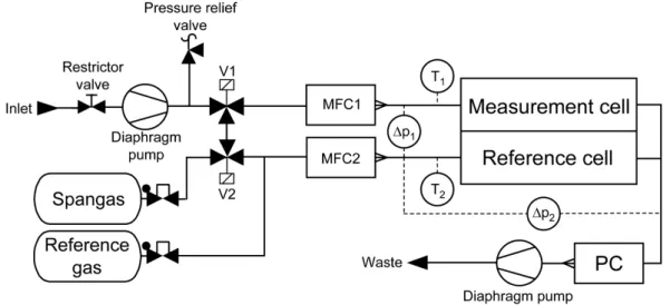
To operate the system on board of a research aircraft and perform high precision measurements, several modifications of the LI-6262 were necessary. In particular, a high precision flow system is required, since both the ambient pressure outside the

20

aircraft and the cabin pressure depend on flight altitude. Figure 1 shows the flow sys-tem built for FABLE. Ambient pressure varies between about 1030 hPa in the boundary layer and less than 200 hPa at the highest flight levels.

Sampling is accomplished via a 1_/₂_{” stainless steel sampling tube pointing into the} flight direction. The sample gas is pressurized to about 1150 hPa by a three-stage

25

Teflon diaphragm-pump (model MD 1 VARIO, Vacuubrand, Germany). A restrictor valve on the low-pressure side of the pump controls the flow in the boundary layer. On the high-pressure side, a pressure relief valve establishes a constant pressure approximately 150 hPa higher than cabin pressure. Via a low ∆p mass flow controller

(6)

ACPD

Full Screen / Esc

Printer-friendly Version Interactive Discussion (MFC 1: Bronkhorst, The Netherlands) the pressure ahead of the measurement cell is

regulated to 850 hPa, while the pressure ahead of the MFC varies between 1150 and 950 hPa as a function of the cabin pressure. The time resolution determined as the time constant for a signal change from 5 to 95% is of the order of 4 s for the system including the constant pressure inlet.

5

The reference cell is purged by a 100 sccm flow of reference gas from a gas tank, at a pressure of 850 hPa regulated via MFC 2, to allow a differential measurement between the two cells held at the same pressure. Since the cell absorption and thus the anal-yser output are non-linear functions of the CO2mixing ratio a multi-point polynominal calibration function has been obtained in the laboratory.

10

In flight, the reference gas is used as a secondary calibration gas which can be added to the measurement cell via valves V1 and V2. Additionally, a second standard (Spangas) is used for in-flight calibrations of the instrument span. Both standards are compared in the laboratory to two primary NOAA reference standards with concentra-tions of 366.34 and 390.11 ppm, respectively.

15

To avoid temperature drifts of the instrument, the whole analyser is mounted in a sealed box that is actively temperature controlled.

The in-flight noise level determined from ambient measurements during periods of low atmospheric variability is about 0.055 ppm (1σ). This noise is a measure for the

short-term precision of the instrument. The long-term precision of FABLE is

addition-20

ally affected by changes in the instrument sensitivity over the flight. It is determined as the reproducibility of the in-flight calibrations that varies from flight to flight between 0.050 and 0.300 ppm (1σ). The calibration accuracy (0.109 ppm, 1σ) is determined by

the in-flight standards. Thus the total uncertainty of the CO2 measurement with FA-BLE is estimated at 0.366 ppm (1σ), roughly 0.1% of the ambient mixing ratio. This

25

corresponds to an improvement by roughly a factor 2 compared to the analyser spec-ifications provided by LI-Cor inc., which is mainly achieved by the temperature and pressure stabilization of the FABLE instrument.

(7)

ACPD

Full Screen / Esc

3 Measurements during SPURT

A total of eight 2-day measurement campaigns covering all seasons were performed within SPURT during the time periods 10–11 November 2001; 17–19 January, 16– 17 May, 22–23 August, and 17–18 October 2002; 15–16 February, 27–28 April, and 9–10 July 2003. Carbon dioxide measurements were obtained during the first 7

cam-5

paigns; for the last one data are missing due to an instrument failure. All campaigns were flown out of the aircraft’s home base Hohn in northern Germany (54◦

N, 9◦ E). A typical campaign consisted of at least two southbound flights within one day, followed by two or more northbound flights performed on the next day. Thus a series of flights covered the latitude range between approximately 35◦ _{and 75}◦_{N along the western}

10

shore of Europe. During stop-over landings at airports in the subtropics (Faro (Portu-gal, 37◦_{N, 8}◦_{W), Casablanca (Morocco, 33}◦_{N, 7}◦_{W), Gran Canaria (28}◦_{N, 15}◦_W), Lis-bon (Portugal, 38◦_{N, 9}◦_{W), Jerez (Spain, 36}◦_{N, 6}◦_{W), Monastir (Tunisia, 35}◦_{N, 10}◦_E), Sevilla (Spain, 37◦_{N, 5}◦_{W)) and at high northern latitudes (Kiruna (Sweden, 68}◦_N, 20◦_{E), Troms ¨o (Norway, 69}◦_{N, 18}◦_{E), Keflavik (Iceland, 64}◦_{N, 22}◦_{W), Longyearbyen}

15

(Norway, 78◦_{N, 15}◦_{E)) two profiles between ground-level and approximately 14 km} al-titude were obtained during landing and take-off (see Fig. 1 of Fischer et al., 2006). Detailed descriptions of the individual campaigns can be found in the overview article by Engel et al. (2006).

4 Results

20

4.1 Comparison with GAW observations

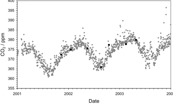
To compare the airborne measurements during SPURT with ground-based obser-vations, Figure 2 shows data from the GAW station Zugspitze (47.25◦_{N, 10.59}◦_E, 2960 m a.s.l.) (data obtained from: http://gaw.kishou.go.jp) as measured by the Ger-man Umweltbundesamt. This site has been chosen because it is considered to be

(8)

ACPD

Full Screen / Esc

Printer-friendly Version Interactive Discussion representative for mid-latitudes where we obtained profiles from the SPURT

measure-ments. To avoid direct contamination at the surface in close proximity to the airports, the comparison is made for a mountain site. Also shown in the figure are SPURT ob-servations from landings and take offs in Hohn, averaged within 1-km thick altitude bins corresponding to the height of the station. The airborne observations closely follow the

5

daily variations at the station and deviations generally do not exceed 1 ppm (mean difference=–0.2 ppmv), which underlines both the accuracy and representativity of the SPURT data.

4.2 Vertical profiles

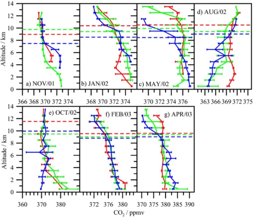
Average profiles of CO2mixing ratios for the individual campaigns are shown in Figure

10

3. Mean values and 1σ-standard deviations for 1 km altitude bins have been calculated

from take-offs and initial ascent as well as during the final descents at high (>65◦ N, blue lines), middle (approx. 55◦_{N, green lines) and subtropical latitudes (}_<40◦_{N, red} lines).

Significant latitudinal variations are observed in the lower layers of the troposphere

15

(below 5 km), in particular during the summer/fall transition (August to October 2002). In the boundary layer below ∼1 km a gradient of about –0.2 ppm/degree latitude is ob-served between 35◦_{N and north of 55}◦_{N during August 2002, maximizing in October} 2002 at about –0.35 ppm/degree latitude between<50◦_{N and 65}◦_{N. These strong} lati-tudinal gradients at low altitudes in summer reflect the enhanced up-take by vegetation

20

during the growing season. This sink is strongest at high latitudes (blue lines in Fig. 3d and e) yielding a CO2profile with lowest concentrations close to the ground. This effect is much smaller at lower latitudes. In the late winter/early spring seasons (in particu-lar during February 2003) when boundary layer mixing ratios are highest, a latitudinal gradient is not discernable.

25

In general, only small seasonal differences between different latitude bands are found in the middle troposphere between 5 and 9 km. Above 9 km in the upper tro-posphere/lowermost stratosphere again significant latitudinal gradients are observed

(9)

ACPD

Full Screen / Esc

Printer-friendly Version Interactive Discussion in particular during the spring season (May 2002 and April 2003). In the tropopause

region these latitudinal differences are mainly related to differences in the tropopause height, with a generally low tropopause at high latitudes and a high tropopause at low latitudes, in particular during the spring season (Fig. 3c and g).

The individual profiles shown in Fig. 3 can be influenced by synoptic transport and

5

mixing, leading to local variations in atmospheric CO2that do not necessarily reflect cli-matological meridional gradients. Thus advection from different latitudes and altitudes may be responsible for at least part of the observed variability in individual profiles (Gerbig et al., 2003).

To study the effect of transport on the individual profiles we used the Lagranto

trajec-10

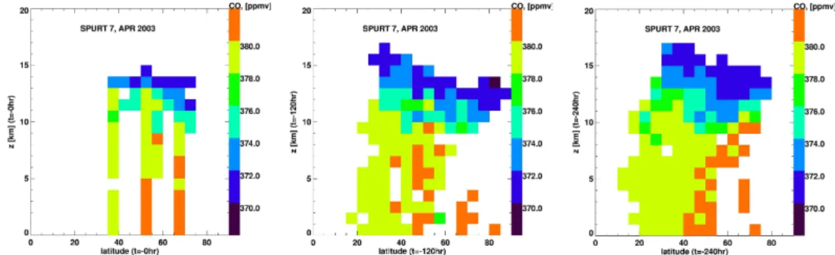
tory model (Wernli and Davies, 1997) to calculate 10-day backward trajectories based on 3-hourly operational ECMWF analysis fields of horizontal and vertical winds. The trajectories were started every 10 s along the flight tracks of each SPURT mission. As an example, Fig. 4 shows all CO₂measurements obtained during SPURT mission 7 in April 2003, averaged in altitude (1 km) and latitude (5◦

) bins. The left panel shows the

15

in-situ observations with the average profiles obtained during take-off and landing at Lisbon (38◦_{N), Hohn (54}◦_{N) and Kiruna (68}◦_{N), as well as the observations in the} up-per troposphere and lowermost stratosphere during the flights between these airports. As in Fig. 3g one can identify a small latitudinal gradient in the lower troposphere, with lowest mixing ratios in the subtropics, as well as local enhancements in the upper

20

troposphere at mid (around 8 km) and high latitudes (between 5 and 7 km).

The middle and right panels of Fig. 4 show the distribution of the measured CO2 values advected backwards to the corresponding altitude and latitude of the sampled air parcels 120 and 240 h back in time, respectively. In particular for the 240 h time period a large-scale ordering of the data appears, with a high-altitude low-stratosphere

25

cluster characterized by CO₂ mixing ratios below 374 ppm, and a weak though clear latitudinal gradient in the troposphere with the highest values toward the high latitudes. Note that a similar structuring has been obtained for all campaigns. In general, the strongest vertical gradients are observed around the tropopause, while the latitudinal

(10)

ACPD

Full Screen / Esc

Printer-friendly Version Interactive Discussion gradients in the troposphere are rather small. We conclude that the variability in the

local profiles in the free troposphere is mainly due to advection from different altitudes and latitudes in synoptic systems.

4.3 Seasonal variations

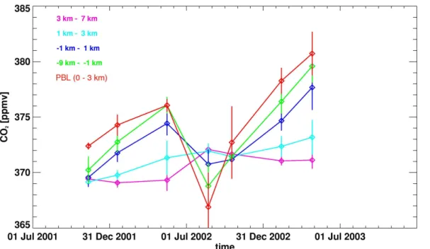
The seasonal variation is illustrated in Fig. 5. Considering that Figs. 3 and 4 show only

5

small latitudinal differences above the boundary layer, all data have been grouped with respect to distance to the local tropopause, defined as the 2 PVU (potential vorticity unit) surface (Hoor et al., 2004), including constant level flight legs and independent of the latitude of observation. For this purpose the data have been averaged for the boundary layer (0–3 km, red line in Fig. 5), the free troposphere (from the boundary

10

layer to 1 km below the tropopause, green line), the tropopause region defined as 1 km below to 1 km above the local tropopause (purple line), the extra-tropical tropopause layer (1 to 3 km above the local tropopause, blue line) and the lowermost stratosphere (3–7 km above the tropopause, pink line).

The CO₂mixing ratios at all atmospheric levels exhibit a temporal trend with

increas-15

ing concentrations from November 2001 to April 2003. This increase is strongest in the lowest three kilometres (∆CO2=4 ppm from January 2001 to February 2002), getting smaller (3.7 ppm) in the free troposphere and smallest in the lowermost stratosphere (∆CO2=2 ppm from 1 to 7 km above the local tropopause).

In addition, a strong seasonal variation is observed. In the boundary layer,

low-20

est mixing ratios are observed during August 2002 after a decrease of 9.3 ppm below the spring maximum, followed by a strong increase of about 11 ppm until December 2002. A similar seasonal variation in phase with the boundary layer concentrations is observed in the free troposphere although with reduced amplitude (∆CO2=–4 ppm and +7 ppm from May 2002 to August 2002 and August 2002 to December 2002,

re-25

spectively). This confirms the model simulations performed by Olsen and Randerson (2004), indicating that column CO2has less variability than surface CO2.

(11)

com-ACPD

Full Screen / Esc

Printer-friendly Version Interactive Discussion plete seasonal cycle. Thus the stated temporal trends – in particular the exact timing

of the extremes in the seasonal variation – could well be spurious and detailed com-parisons with seasonal variations of CO2at ground-based sites are difficult.

As already mentioned by Hoor et al. (2004) the seasonal variation differs between the lowermost stratosphere and the troposphere. Contrary to a local maximum in spring

5

and a minimum in summer found in the troposphere, CO2mixing ratios in the lowermost stratosphere exhibit a pronounced maximum in summer and a broad minimum in winter and spring. The amplitude of the seasonal variation in the lowermost stratosphere is ∼3 ppm, slightly lower than found in the free troposphere and phase shifted by approx. 3 months, in agreement with observations by Nakazawa et al. (1991). According to Hoor

10

et al. (2004) this phase lag is due to longer transit times for the tropospheric fraction of air mixed into the lowermost stratosphere, and likely a different transport pathway. For a detailed discussion of the CO2 seasonal cycle in the lowermost stratosphere and its relationship to cross-tropopause transport the reader is referred to Strahan et al. (1998), Hoor et al. (2004, 2005) and Strahan et al. (2007).

15

4.4 Comparison to a Marine Boundary Layer Reference

Next we investigate the difference between the free tropospheric CO2 values and mixing ratios observed in the marine boundary layer (MBL reference) (Masarie and Tans, 1995). The MBL reference includes longitudinally averaged observations within the marine boundary layer as a function of time (weekly values) and sine of latitude

20

(GLOBALVIEW 2006 data products are available at http://www.esrl.noaa.gov/gmd/

ccgg/globalview/). Considering the absence of direct observations and for comparison purposes we use the MBL reference also for the free troposphere (Lin et al., 2006).

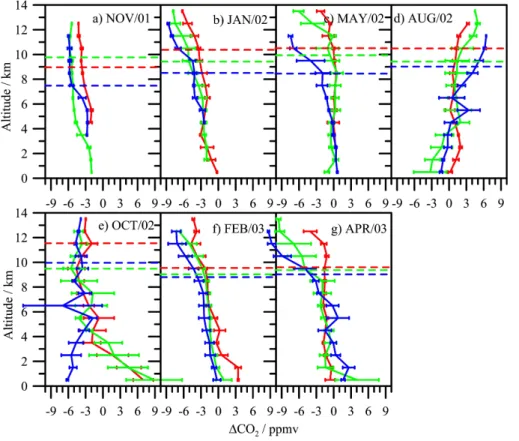
In Figure 6 the difference ∆CO2between CO2(SPURT) and CO2(MBL) is plotted as a function of altitude for the SPURT profiles obtained during the 7 campaigns. In the

25

boundary layer (below 3 km) ∆CO2is small during winter and spring (less than 3 ppm), while larger deviations are observed during summer at middle and high latitudes, a signature of strong uptake by the vegetation. SPURT measurements at high latitudes

(12)

ACPD

Full Screen / Esc

Printer-friendly Version Interactive Discussion during October 2002 are still ∼6 ppm lower than the MBL reference, a remainder of the

summertime biosphere sink. In contrast, mixing ratios at middle and low latitudes are higher than the MBL reference by 6–9 ppm. Probably this is due to local emissions in the proximity of airports, typically located in populous regions.

Above the boundary layer we find a gradual decrease of ∆CO2with altitude, in

par-5

ticular during the fall and winter seasons. These negative values extend into the lower-most stratosphere, were lowest values up to –9 ppm are reached. The ∆CO2-altitude gradient reverses in summer, with increasing values of ∆CO2up to +3 ppm above the tropopause. In spring, during the transition from negative to positive gradients, ∆CO2is negligible throughout the troposphere and only slightly negative in the lowermost

strato-10

sphere, in particular at low and middle latitudes. Systematic deviations between free tropospheric observations and the MBL reference have been explained in the literature by advection from different latitudes and time lags related to the vertical propagation of concentration changes from the surface to the free troposphere (Gerbig et al., 2003).

The near-continual decrease of ∆CO2 with altitude in fall and winter, as well as the

15

steady increase during summer could also be caused by the influence of stratosphere-troposphere transport (STT) on the vertical profiles (Sawa et al., 2004; Shia et al., 2006). In the fall and winter seasons the enhanced downward transport (compared to the summer season) of aged CO2-poor air from the stratosphere yields lower values of CO₂ in the upper troposphere relative to the MBL reference (∆CO2<0). Thus the

20

∆CO2-altitude relation follows a mixing line between a CO2-poor stratospheric reser-voir and the MBL reference. Since the influence of STT on trace gas concentrations decreases with distance from the tropopause, ∆CO2declines to zero at lower altitudes. In summer the situation reverses due to the higher CO2concentrations in the strato-sphere relative to the MBL reference (∆CO2>0), yielding higher ∆CO2 in the UT and

25

zero in the middle and lower troposphere. In spring, when altitude gradients are weak, the signature of STT is negligible, since the mixing line connects reservoirs with similar CO2mixing ratios in the stratosphere and troposphere.

(13)

dur-ACPD

Full Screen / Esc

Printer-friendly Version Interactive Discussion ing SPURT (not shown). Fischer et al. (2006) compared the observed CO and O₃

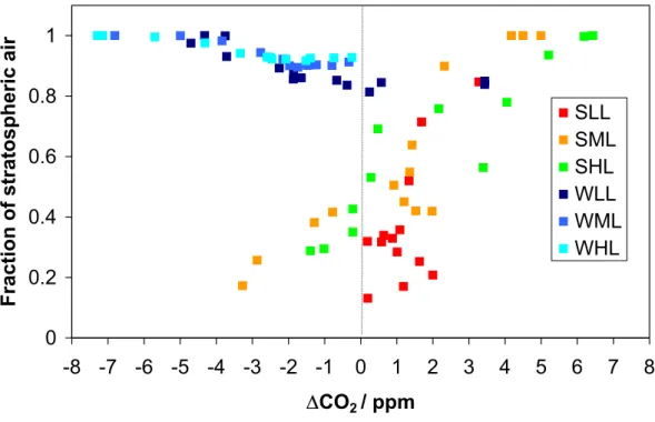
profiles to 3D-chemical transport model (CTM) simulations by the MPI-C Model for At-mospheric Chemistry and Transport (MATCH-MPIC) (Lawrence et al., 2003). A tracer for stratospheric O₃ calculated in the model can be used to estimate the contribution of stratospheric ozone to the O3 burden in the troposphere. In Figure 7 this fraction

5

(modelled stratospheric O3/modelled total O3) has been plotted versus ∆CO2 for the summer and winter seasons, respectively. Both seasons show a significant linear re-lationship. The strongest correlations are found at middle and high latitudes (R2>0.8),

while weaker correlation coefficients are deduced for low latitudes (R2 between 0.4 and 0.6). This finding from the model simulations supports the interpretation that the

10

observed altitude gradients of ∆CO2are most likely due to STT.

5 Summary and conclusions

In the present work we describe airborne CO₂ measurements over Western Europe covering altitudes from the planetary boundary layer up to the lowermost stratosphere and latitudes from the Artic to the sub-tropics. These measurements have been

per-15

formed during all seasons as part of the SPURT project between November 2001 and April 2003. With the exception of summer all seasons have been probed twice. In addition to latitudinal gradients in the upper troposphere and lowermost stratosphere, ascents and descents into airports at high (>65◦

N), middle (∼55◦_{N) and subtropical} (<40◦

N) latitudes provided data on vertical gradients over generally small, low-duty

20

airports. This allows a comparison of the seasonal variation of CO2 in the continental boundary layer (CBL), the free troposphere and the region above the local tropopause at different latitudes.

As expected, seasonal variations and latitudinal gradients are largest in the CBL, re-flecting the role of surface sources and sinks. The strongest changes are due to the up

25

take by vegetation, which maximizes in late summer, resulting in inverted profiles with increasing concentrations with altitude. During the other seasons CO2 tends to

(14)

de-ACPD

Full Screen / Esc

Printer-friendly Version Interactive Discussion crease with altitude. In the free troposphere, seasonal as well as latitudinal variations

typically have a strongly reduced amplitude compared to the CBL. The comparison of our measurements to a marine boundary layer reference obtained from the GLOB-ALVIEW data indicates that the damping of the free tropospheric seasonal cycle and latitudinal gradients are due to mixing with aged air masses, most probably transported

5

down from the lowermost stratosphere. Directly above the tropopause, i.e. in the extra-tropical tropopause layer, the seasonal cycle is in phase with the upper troposphere, but deeper into the stratosphere it is phase-shifted by approximately 3 months, indicating transport of aged air from the overworld mixed with air masses horizontally transported from the tropics, as suggested by Hoor et al. (2004, 2005).

10

As a final note, the data presented in this paper is freely available from the SPURT server (http://www.iac.ethz.ch/staff/dominik/spurt/index.html) after signing the data protocol. These data could be of value in inverse modelling and satellite validation studies.

Acknowledgements. We acknowledge funding from the German Ministry for Education and

15

Research BMBF under the AFO2000 Program. We thank the Learjet team (enviscope and GFD) for excellent cooperation during the field campaigns. HW thanks Meteo Swiss for granting access to operational ECMWF data.

References

Anderson, B. E., Gregora, G. L., Collins Jr., J. E., Sachse, G. W., Conway, T. J., and Whitin, G.

20

P.: Airborne observations of spatial and temporal variability of tropospheric carbon dioxide, J. Geophys. Res., 101, 1985–1997, 1996.

Aoki, S., Nakazawa, T., Machida, T., Sugawara, S., Morimoto, S., Hashida, G., Yamanouchi, T., Kawamura, K., and Honda, H.: Carbon dioxide variations in the stratosphere over Japan, Scandinavia and Antarctica, Tellus 55B, 178–186, 2003.

25

Barkley, M. I., Monks, P. S., and Engelen, R. J.: Comparison of SCIAMACHY and AIRS CO₂ measurements over North America during the summer and autumn of 2003, Geophys. Res. Lett. 33, L20805, doi:10.1029/2006GL026807, 2006.

(15)

ACPD

Full Screen / Esc

Boering, K. A., Wofsy, S. C., Daube, B. C., Schneider, J. R., Loewenstein, M., Podolske, J. R., and Conway, T. J.: Stratospheric mean ages and transport rates from observations of CO₂ and N₂O, Science, 274, 1340–1343, 1996.

Buchwitz, M., de Beek, R., N ¨oel, S., Burrows, J. P., Bovensmann, H., Bremer, H., Bergam-aschi, P., K ¨orner, S., and Heimann, M.: Carbon monoxide, methane and carbon dioxide

5

total columns retrieved from SCIAMACHY by WFM-DOAS: Year 2003 initial data set, Atmos. Chem. Phys. 5, 3313–3329, 2005.

Chedin, A., Serrar, S., Scott, N. A., Crevosier, C., and Armante, R.: First global measure-ments of midtropospheric CO₂from NOAA polar satellites: Tropical zone, J. Geophys. Res., 108(D18), 4581, doi:10.1029/2003JD003439, 2003.

10

Daube, B. C., Boering, K. A., Andrews, A. E., and Wofsy, S. C.: A high-precision fast-response airborne CO₂ analyzer for in-situ sampling from the surface to the middle stratosphere, J. Atmos. Ocean. Techn., 19, 1532–1543, 2002.

Engel, A., B önisch, H., Brunner, D., Fischer, H., Franke, H., G ünther, G., Gurk, C., Hegglin, M., Hoor, P., K önigstedt, R., Krebsbach, M., Maser, R., Parchatka, U., Peter, T., Schell, D.,

15

Schiller, C., Schmidt, U., Spelten, N., Szabo, T., Weers, U., Wernli, H., Wetter, T., and Wirth, V.: Highly resolved observations of trace gases in the lowermost stratosphere and upper troposphere from the Spurt project: an overview., Atmos. Chem. Phys., 6, 283–301, 2006,

http://www.atmos-chem-phys.net/6/283/2006/.

Engelen, R. J. and McNally, A. P.: Estimating atmospheric CO₂from advanced infrared satellite

20

radiances within an operational fourdimensional variational (4D-VAR) data assimilation sys-tem: Results and validation, J. Geophys. Res. 110, D18305, doi:10.1029/2005JD005982, 2005.

Fischer, H., Lawrence, M., Gurk, C., Hoor, P., Lelieveld, J., Hegglin, M., Brunner, D., and Schiller, C.: Model simulations and aircraft measurements of vertical, seasonal and latitudinal

25

O₃and CO distributions over Europe, Atmos. Chem. Phys., 6, 339–348, 2006,

Hoor, P., Gurk, C., Brunner, D., Hegglin, M. I., Wernli, H., and Fischer, H.: Seasonality and extend of extratropical TST derived from in-situ CO measurements during SPURT, Atmos. Chem. Phys., 4, 1427–1442, 2004,

30

Hoor, P., Fischer, H., and Lelieveld, J.: Tropical and extratropical tropospheric air in the low-ermost stratosphere over Europe: A CO-based budget, Geophys. Res. Lett., 32, LO7802,

(16)

ACPD

Full Screen / Esc

doi:10.1029/2004GL022018, 2005.

Gerbig, C., Lin, J. C., Wofsy, S. C., Daube, B. C., Andrews, A. E., and co-authors: Toward constraining regional-scale fluxes of CO₂ with atmospheric observations over a continent: 1. observed spatial variability from airborne platforms, J. Geophys. Res., 108(D24), 4756, doi:10.1029/2002JD003018, 2003.

5

Intergovernmental Panel on Climate Change, Climate Change: The scientific basis. Contribu-tion of working group 1 to the third assessment report of the Intergovernmental Panel on Climate Change (IPCC), edited by: J. T. Houghton et al., Cambridge University Press, New York, USA, 2001.

Keeling, Ch. D.: Rewards and penalties of monitoring the earth, Ann. Rev. Energy Environm.

10

23, 25–82, 1998.

Lawrence, M. G., Rasch, P. J., von Kuhlmann, R., Williams, J., Fischer, H., de Reus, M., Lelieveld, J., Crutzen, P. J., Schultz, M., Stier, P., Huntrieser, H., Heland, J., Stohl, A., Forster, C., Elbern, H., Jakobs, H., and Dickerson, R. R.: Global chemical weather forecasts for field campaign planning: Predictions and observations of large-scale features during MINOS,

15

CONTRACE, and INDOEX, Atmos. Phys. Chem., 3, 267–289, 2003.

Lin, J. C., Gerbig, C., Wofsy, S. C., Daube, B. C., Matross, D. M., Chow, V. Y., Gottlieb, E., Andrews, A. E., Pathmathevan, M., and Munger, J. W.: What have we learned from intensive atmospheric field programmes of CO₂?, Tellus, 58B, 331–343, 2006.

Machida, T., Kita, K., Kondo, Y., Blake, D., Kawakami, S., Inoue, G., and Ogawa, T.: Vertical

20

and meridional distributions of atmospheric CO₂mixing ratios between northern midlatitudes and southern subtropics, J. Geophys. Res., 108, 8401, doi:10.1029/2001JD000910, 2002. Matsueda H. and Inoue, H. Y.: Measurements of atmospheric CO₂and CH₄using a commercial

airliner from 1993 to 1994, Atmos. Environm., 30, 1647–1655, 1996.

Matsueda, H., Inoue, H. Y., and Ishii, M.: Aircraft observations of carbon dioxide at 8-13 km

25

altitude over the western Pacific from 1993–1999, Tellus 54B, 1–21, 2002.

Masarie, K. A. and Tans, P. P.: Extension and integration of atmospheric carbon dioxide data into a globally consistent measurement record, J. Geophys. Res., 100, 11 593–11 610, 2006. Nakazawa, T., Miyashita, K., Aoki, S., and Tanaky, M.: Temporal and spatial variations of upper

tropospheric and lower stratospheric carbon dioxide, Tellus, 43B, 106–117, 1991.

30

Olson, S. C. and Randerson, J. T.: Differences between surface and column atmo-spheric CO₂ and implications for carbon cycle research, J. Geophys. Res., 109, D02301, doi:10.1029/2003JD003968, 2004.

(17)

ACPD

Full Screen / Esc

Pearman, G. I. and Beardsmore, D. J.: Atmospheric carbon dioxide measurements in the Aus-tralian region: Ten years of aircraft data, Tellus, 36B, 1–24, 1984.

Sawa, Y., Mtsueda, H., Makino, Y., Inoue, H. Y., Murayama, S., Hirota, M., Tsutsumi, Y., Zaizen, Y., Ikegami, M., and Okada, K.: Aircraft observations of CO₂, CO, O₃and H₂over the North Pacific during the PACE-7 campaign, Tellus, 56B, 2–20, 2004.

5

Shia, R.-L., Liang, M.-C., Miller, C. E., and Yung, Y. L.: CO₂ in the upper tropo-sphere: Influence of stratosphere-troposphere exchange, Geophys. Res. Lett., 33, L14814, doi:10.1029/2006GL026141, 2006.

Strahan, S. E., Douglass, A. R., Nielsen, J. E., and Boering, K. A.: The CO₂seasonal cycle as a tracer of transport, J. Geophys. Res., 103, 13 729–13 741, 1998.

10

Strahan, S. E., Duncan, B. N., and Hoor, P.: Observationally derived transport diagnostics for the lowermost stratosphere and their application to the GMI chemistry and transport model, Atmos. Chem. Phys. Discuss., 7, 1449–1477, 2007,

http://www.atmos-chem-phys-discuss.net/7/1449/2007/.

Taylor, F. W.: Elementary Climate Physics, Oxford University Press, Oxford, UK, 2005.

15

Tiwari, Y. K., Gloor, M., Engelen, R. J., Chevallier, F., R ¨odenbeck, C., K ¨orner, S., Peylin, P., Braswell, B. H., and Heimann, M.: Comparing CO₂ retrieved from Atmospheric Infrared Sounder with model predictions: Implications for constraining surface fluxes and lower-to-upper troposphere transport, J. Geophys. Res., 111, D17106, doi:10.1029/2005JD006681, 2006.

20

Vay, S. A., Anderson, B. E., Conway, T. J., Sachse, G. W., Collins Jr., J. E., Blake, D. R., and Westberg, D. J.: Airborne observations of tropospheric CO₂ distribution and its controlling factors over the South Pacific Basin, J. Geophys. Res., 104, 5663–5676, 1999.

Wernli, H. and Davies, H. .: A Lagrangian-based analysis of extratropical cyclones. I: The method and some applications, Quart. J. Roy. Meteor. Soc., 123, 467–489, 1997.

25

World Meteorological Organization, Greenhouse Gas Bulletin, No., 2, 2006.

Zahn, A., Neubert, R., Maiss, M., and Platt, U.: Fate of long-lived trace species near the Northern Hemisphere tropopause: Carbon dioxide, methane, ozone, and sulfur hexafluoride, J. Geophys. Res., 104, 13 923–13 942, 1999.

(18)

ACPD

Full Screen / Esc

(19)

ACPD

Full Screen / Esc

Printer-friendly Version Interactive Discussion 355 360 365 370 375 380 385 390 395 400 2001 2002 2003 2004 Date C O2 / p p m

Fig. 2. Comparison of mean airborne observations from SPURT (black symbols) with daily

(20)

ACPD

Full Screen / Esc

Fig. 3. Means and 1σ-standard deviation for 1 km altitude bins calculated from take-offs and

landings at high (>65◦_{N, blue lines), middle (approx. 55}◦_{N, green lines) and subtropical}

(21)

ACPD

Full Screen / Esc

Fig. 4. Meridional cross-sections of CO₂observations from SPURT mission 7 in April 2003 in 5◦_{latitude and 1 km altitude bins. The left panel shows the in-situ observations while the middle}

and right panels show the calculated CO₂distributions 5 and 10 days back in time, respectively, based on 10-day backward trajectories.

(22)

ACPD

Full Screen / Esc

Fig. 5. Seasonal variation of CO₂mixing ratios in different atmospheric altitude sections relative to the 2-pvu tropopause and in the planetary boundary layer at the measurement locations.

(23)

ACPD

Full Screen / Esc

Fig. 6. Vertical profiles of the differences between measured CO2 and the marine boundary

layer reference value at the same latitude (obtained from GLOBALVIEW-CO2 2006 data set) at high (>65◦_{N, blue lines), middle (approx. 55}◦_{N, green lines) and subtropical latitudes (}_<40◦_N,

(24)

ACPD

Full Screen / Esc

0

0.2

0.4

0.6

0.8

1 -8 -7 -6 -5 -4 -3 -2 -1

0

1

2

3

4

5

6

7

8 ΔCO

2

/ ppm

F

ra

c

ti

o

n

o

f

s

tr

a

to

s

p

h

e

ri

c

a

ir

SLL

SML

SHL

WLL

WML

WHL

Fig. 7. Fraction of modelled stratospheric O₃ to the modelled total O₃ versus ∆CO2 for the

summer (S) and winter (W) seasons, respectively. The data are further subdivided into low latitudes (LL), mid latitudes (ML) and high latitudes (HL).