Dissolved Nutrient-Seawater Density Correlations
and the Circulation in
Boston Harbor and Vicinity by
Joseph Karpen
B.A., University of Washington 1972
SUBMITTED IN PARTIAL FULFILLMENT OF THE REQUIREMENT FOR THE
DEGREE OF MASTER OF SCIENCE at the Massachusetts Institute of Technology September, 1973 Signature of Author epartment of Mletorology August 13, 1973 Certified by Accepted by / , Thesis Supervisor
Ch4frman, Departmental Committee on Graduate Students
Lindgren
MIT LS
,
Dissolved Nutrint-Si awatar ,2e tv iCorrelat ins
and the Ciczulation in 3oston Harbor and Vicinity by
Joseph Karpen
Submitted to the Department of Meteoroogy on August 13, 1973 in partial fulfillment of the requirements for the degree of
Master of Science
Abstract
The general circulation between Boston Harbor and Massachusetts Bay was studied from the basis of a tidal exchange problem.. The
Deer Island Sewage Treatment Plant effluent outfall, located at
the mouth of the harbor, was used as a tracer of harbor water. An exchange theory using simplifiad jet and : ink flows was
developed to predi& t-.the effluent concentrations in the har-bor. A correlation between dissolved nutrient concentrations and sigma-t (density) was postulated.
Five cruises were undertaken to verify t',e theory presented; hydrographic stations were made using a Conductivity-Temperature-Depth (CTD) sensor -package, and water samples were taken to
measure dissolved nutrient concentrations. Wind induced surface
and possible geostrophic currents were noted as other sources of flow.
A significant correlation was found between dissolved nutrient concentrations and sigma-t. It appears the harbor water mass
moves seaward into Massachusetts Bay as a larre, fairly
homogenous volume, "blob", a new blob moving into the bvy on
each ebb tide. Further avenues of study are mentioned, especiaily with respect to the movement of the harbor water into -the bay.
Thesis Snoerv-isor: Erik Moll-Christe sen
Acknow!.ed amen t
I espci i a1l thank E. .io--Chnr stensen, P. Rhines, and H. Stommel for their help and suggestions, B. Beardsley while
E. M-C. was not available, B. Laird who aided writh the computer
programs and programming. K. Kim was in charge of collecting the August data, D..-Strimaitas, E. Sambuco and others who crewed for the other cruises. (Also, E. Sambueo took the photographs of the Deer Island Plume). S. Frankel aided with the chemistry
determinations. Thanks to those not named, but who also helped. I especially want to thank my wife Susan for her patience and understanding while this report was being written. (She also wrote in all the equations.)
Funds for this project and report came in part from the Henry L. and Grace Doherty Charitable Foundation, Inc. grant to M.I.T. Seagrant as well as from Seagrant #NG-43-72 from the NOAA
Office of Seagrant, U.S. Dept. of Coummerce and the National Science ?oundation grant #GA-30729X
TABLE OF CONTENTS Page Title 1 Abstract 2 Acknowledgements 3 List of Tables 5 List of Symbols 6 Chapter 1 Introduction 8 Chapter 2 Theory 12 2.1 Preliminary 12
2.2 Tidal Exchange Problem 15
2.3 Discussion 20
2.4 Dissolved Nutrient - Sigma-t Correlations 22
2.5 Linear Regression 24
Chapter 3 Data Presentation and Analysis 26
3.1 Deer Island and River Flows 26
3.2 Estimate of Dissolved Nutrient Concen- 28 trations from Theory
3.3 Field Observations 30
3.3.1 Methods of Data Collection 30
3.3.2 Cruise 1 32
3.3.3 Use of Only Sigma-t 34
3.3.4 Cruise 6 35
3.3.5 Cruise 7 35
3.3.6 Cruise 8 36
3.3.7 Cruise 9 37
3.3.8 Aerial Observations 40
3.3.9 Wind Induced Surface Currents 40 3.4 Dissolved Nutrient - Sigma-t Correlations 42
3.5 Sample Regression 42
Chapter 4 Results 44
4.1 Release of "Blobs" 44
Chapter 5 Summary and Conclusions 46
References 49
LIST OF TABLES
Table Page
lA
Monthly Average River and Deer Island 51Effluent Flows
lB
Spot Once-a-Month Effluent Chemical 52Concentrations
2 Predicted Values of Dissolved Nutrient 53
Concentrations in Boston Harbor from Theory
3A Station 21, Cruise 9 Specific Volume Anomaly 54 3B Station 22, Cruise 9 Specific Volume Anomaly 55 3C Geostrophic Current from Field of Mass, 56
Stations 21 and 22
4 Wind Induced Surface Currents 57
5 Correlations between Dissolved Nutrient 58
Concentrations and Sigma-t
-5-Symbol b C, C(I), C K, K'
Q
Q'
r r xy R1 R2 t tl u Uo Vo Vl, V2, V3, V4, V5 w x LIST OF SYMBOLS Definition Half width of an openingA concentration of dissolved nutrients or pollutants
Depth of upper mixed layer
Diffusivity of dissolved nutrients Dissolved nutrient or pollutant flux
(a concentration times a volume flux) Integration constants
Flux through harbor opening
Two dimensional flux through harbor opening
Radial distance from harbor opening Sample correlation coefficient Extent of sink flow region Length of tidal excursion Time
Time of half a tidal period Velocity
Half tidal cycle average velocity Wind induced surface current velocity
Tidal exchange volumes, see Figure 4 Wind velocity
Measured value of Concentration
Dimensions L L L2/T L3/T L /T L3/T L2/T L2 L L T T L/T L/T L/T 3 L/T
x Predicted value of concentration
y Measured value of sigma-t
Probability of accepting a false hypothesis
6 Anomaly of specific volume L3/M
0 Angle of opening
P1' P2 Density M/L
3
Pxy Correlation coefficient
Te.f. e-folding time (tidal cycles)
T(I) Tidal period number
Latitude
-7-CHAPTER 1 INTRODUCTION
From the history of man, main areas of civilization have
developed along coasts and on rivers. The local waters were used as convenient waste disposal areas; when populations were small, there was no noticeable effect on the quality of the local waters. The
process of urbanization and industrialization has led to the develop-ment of large population centers along the coastlines, and the
continued disposal of wastes in the local waters. As a result of this concentration of wastes in the near shore areas, they have become the "septic tank of the megalopis" (DeFalco, 1967). A report by Hydroscience, Inc. (1971) on the quality of the waters in Boston
Harbor indicates the particularly poor situation that existed there prior to 1968 when the Deer Island Sewage Treatment Plant went into full operations.
Increasing population pressures make it necessary that a continu-int study be done of the physical factors involved in coastal processes, to prevent pollution of our coastal zones. Of extreme importance is the circulation of the coastal waters and their movement of the waste materials of man from the coast out to sea.
Taylor's (1960) theory of diffusion by continuous movements formed the basis for the early work in dispersion of pollutants in water. The concept of tidal prisms was used by Ketchum (1951) to calculate the mix-ing of salt and fresh waters in tidal estuaries. Aarons and Stommel
A similarity solution for estuarine circulation was developed by Rattray and Hansen (1962). Bowden (1967) presents an overview of work done to that time, with emphasis on vertical and longitudinal circulation. A review of estuarine modeling by Overland (1972) covers advances from 1967 to 1972, and also includes an estuarine type classification system. Stommel and Farmer (1952) and Pritchard (1967) have given similar
estuarine classifications.
Fischer (1972) includes transverse transport in his model for mass transport in estuaries. He presents the idea "that a net transverce circulation may be induced by the interaction of tidal currents with the boundary geometry. The simplest example would be a flow through a small entrance into a circular basin, the flow enters as a jet and leaves as a potential sink, implying a net circulation inward along the diameter and outward along the edges". Stommel (1972) suggests this model might also fit the circulation between Boston Harbor and Massachusetts Bay; the water enters Massachusetts Bay as a jet (ebb tide), and on the flood
tide flows into the harbor as a potential sink.
A simple theory for the dispersion of a source located at the
mouth of Boston Harbor using jet and sink flow is developed in the follow-ing sections. Field work was undertaken to 1) determine the actual dis-tribution of a source of dissolved nutrients (the Deer Island Treatment Plant effluent), 2) verify the dispersion theory and 3) determine if it is feasible to specify what the dissolved nutrient distribution should be by measuring the density distribution.
-9-NEW HA M P SHIRE
ATLANTIC
OCEAN
HARBOR MAS S. BAY MASSACHUSETTS APE COD TUCKET SOUNDao
0
4zz
SCALE! NAUTICAL MILES 0 1/2 MYSTIC R. S / I L e, l' kI ENT
1u' BOSTON HARBOR STUDY
LOCAL AREA CHART
0 DISCHARGE LOC A T.ION
BROAD SOUND EER 1. MASS.BAY MASS. BAY 700 50' Figure 2 ~asU~~
CHAPTER 2 THEORY
2.1 Preliminary
The area of study is Boston Harbor and the area of Massachusetts Bay adjacent to the harbor (Figure 1). The Deer Island Treatment Plant outfall, the source of dissolved nutrients to be used to study the harbor
circulation, is located at the mouth of the harbor, just east of President Roads (Figure 2). The effluent is assumed to rise to the
surface, where it then mixes with the harbor water to a depth of three to four meters. On this basis, the flow theory to be developed will be based on two dimensional jet and sink theory.
The ebb tidal flow into the Bay is assumed to be a jet, the flood tidal flow from the Bay is a potential sink. Conversely, the ebb tidal flow from the harbor is assumed to be a potential sink, and the flood tidal flow is a jet into the harbor. Coriolis effects are neglected, and the time scale for significant diffusion is assumed to be greater than a tidal period, the scale of the process being studied.
The conversion of dissolved solids can be expressed as aC
DV.(VC) = -- + P'VC
at where
.*VC
is the advective term and - DV.(VC)
- 5 2
D z1 x 10 cm /sec (Phillips, 1969), u = 50 cm/sec, and the length scale L of order 104 cm, the advective term is approximately 1010
greater than the diffusive term. Biological activity, especially with reference to the large spring and somewhat smaller fall bloom, is neglected as to its effects on the concentration of the dissolved nutrients.
The ebb flow has a half tidal cycle average velocity Uo, through 2
an opening half width b (Figure 3). Uo is defined as - x maximum tidal velocity.
2b
Figure 3
With a half tidal period of time tl, the distance a parcel of water starting at the opening can travel during time tl is
R2 = Uo tl
The volume of water flowing through the opening is thus V2 = 2bd R2 = Uo 2bd tl
where d is the depth of the upper mixed layer. If Q' is the flux through the opening, V2 = Q'tld
-13-For the flood tide, let R1 be the maximal radial distance from the opening for a particle to pass through the opening during a flood tide. Let 0 be the angle of the opening for this potential sink. A water parcel in a potential sink has its radial velocity determined by
ar. -Q,
at
Or
where Q', the flux through the opening is defined by
Q' ar rdO'.
at
Integrate from time t from the Bay) to time
(r=0) t=tl
r-at (r=Rl) t=0 2 (R1) = Q'tl 2 0
= 0, slack water, through flood tide (for flow t = tl, high water. t=tl dt = - Q' dt t=0 Rl = (2Qtl)1/2 but Q't1 = 2bR2 R bR2 1/2
R1 = 2(
)
Thus, for a fixed half opening width b,
R1
a
(R2)1
/ 2and note that R2 varies with changing Uo. At the mouth of Boston
ebb velocity varies from 0.20 to 0.66, with a mean of 0.43 meters per second. An ebb velocity of 0.66 meters per second does not necessarily mean the preceding or following flood velocity was 0.75 meters per
second. The tides are semi-diurnal with the maximum velocities occuring around the time of the spring tides.
Assume the tides in the harbor have no daily variation in height. Then from conservation of mass equal volumes of water are exchanged between the harbor and the bay on each tidal cycle. Thus V2 is also the volume of the sink flow water, and letting Vl be the volume of the jet water which is not part of the sink flow (Figure 4)
bR2 1/2 d
Vl = 2bd Rl = 4b ( ) d V2 = 2bd R2
The ratio of the volumes V1 2 b )1/2
V2 GR2
indicates that for a fixed b, an increase in R2 (e.g. Uo) implies a smaller ratio of Vl/V2. As will be shown later, the ratio Vl/V2 can be thought of as a "sink flushing number". The half width b is assumed to be much less than R2 in order to haintain the assumption of uniform potential sink flow, i.e., a point sink.
2.2 Tidal Exchange Problem
Assume the initial concentration in the harbor of a dissolved
nutrient is C(I) at low water. The dissolved nutrient concentration just outside of the harbor mouth of an ebb tide is the sum of the concentra-tion in the harbor and the pollutant flux at the harbor mouth, diluted by the tidal flux and volume flux of the source. Assume the volume
-15-E
flux of the source is much less than the tidal flux, << 1. Then E +
C (I) ~~
E+
C(I)
E+Q
Q
where E is a constant flux of pollutants at the harbor mouth and
Q = Q'd
Figure 4
On the flood tide, the water returns to the harbor with a concentration
(E + C(I)) Vl +E
Q
V2
Q
where the first term is the dilution of the dissolved nutrient
concentration with the "clean" water in the bay, and E/Q is the diluted pollution flux as before. From conservation of mass, equal volumes of water are exchanged between the harbor and the bay on each tidal cycle. Assume, also, the nutrients in the harbor volume V5, will not contri-bute to the low water concentration in the harbor since they will be removed on the next ebb tide. Thus, the concentration in the harbor
the water in the harbor is completely and uniformly mixed. On the next flood tide, the inflowing water has concentration
E VI E
( + C(I+1))V- +
Q
V2
Q
The dissolved nutrient concentration in the harbor is now
C(I+1)V3 E Vl V4-V5 E V4-V5
C(I+2) V3+V4 + ( + C(I+1)) V3+V4 +
V3+V4
Q
V2 V3+V4
Q V3+V4"
The difference in concentrations over a tidal period T(I+1) - T(I) C(I+)-C(I) = C( V4V2-Vl(V4-V5) E V2(V4-V5)+V1(V4-V5)
T(I+1)- (I) (V3+V4) V2 Q V2(V3+V4)
AC(I)
Assume a steady state situation, so that =(I) 0.E (V2+Vl)(V4-V5) C(I) =
-Q V2V4-Vl(V4-V5)'
From conservation of mass, and assuming a constant half tidal cycle average velocity, neglecting the volume of the E flux,
E - << i, VI = V5 and V2 = V4
Q
so 2 2 E (V2) - (Vl) C(I) + Q (V2) 2+(Vl) 2-VV2 Expand in a Taylor series,C(I) E 1 V1 2 1
S 1- V V1 2 V2 V1 (V1 2
E
[1
+
v
Vl V2 V 3 V1 4(
- (
)
+(-)
1
Q
V2
V2
V2
V2
Assume the dissolved nutrient concentration of the water returning to the harbor on a flood tide has been diluted by the bay water, VI/V2 < 1. Then as a rough approximation
E V1
C(I)
-
-(1 + )
Q
V2
-17-for a steady state situation. Note that -17-for VI of order V2 the assump-tions of point sink flow and dilution of the pollutants are violated.
Going back to the differential equation for C(I), and also again assuming a constant half tidal cycle average velocity, integrate and look for the time development to a steady state.
AC(I) E AT(I= - C()A + Q where 2 2 (V2) + (Vl) - VIV2 4 V2(V2 + V3) and (Vl+V2) (Vl-V2) A+ V2(V3+V4) Then AT(I) 1
AC(I) -C(I)A4 + E/Q A
1 1
A4 C(I) - (E/Q)(AlA4) Integrate, using indefinite integrals
fdT(I) = fl dC(I) + K
A4 C(I) + (E/Q)(A/A4) 1
T(I) = In[C(I) + (E/Q)(A/A4)] + K A4
C(I) = K'exp[-A4T] + E A Q A4"
Assume that at time T(I) = 0 (no tidal cycles have elapsed, thwer T(I) is the number of tidal cycles), C(I) = 0. Then the integration constant K' is EA K' = Q A4' Thus
2
2
2
2
Note here that C(I) approaches a steady state concentration asymptotically. Letting T(I) * co
2 2
Lim C(I) E (V2) -(Vi) ~ E Vl (V2) + (Vi) -VlV2
T(I)
-Notice this is the same solution derived by assuming a steady state situation from the differential equation.
The e-folding time, Te.f., is a measure of how fast a system moves towards an asymptotic value. Te.f. is defined as the time required for the dissolved nutrient concentration to reach l/e times its asymptotic or steady state concentration.
1 C(I) =-C
e s
where C is the asymptotic value of C(I). s 1 -1= - exp (-A4 T ) e e.f. 1 In(l- -) = - Ar T e e.f. 1 1 T - In(l - -) e.f. A4 e 1 T = 0.458-e.f. A4 V2(V2+V3) T = 0.458 ( V2(V2V) e.f. 2 2 (V2) + (Vi) -VIV2
Again expanding a Taylor series and assuming Vl/V2 < 1,
T = 0.458[ 1 + V-( 1 e.f. Vl VI 2 V2 V+ Vl 2 1-( +()) 1-( +()) V2 V2 V2 V2 V3 Vl Vi Tf 0. 4 5 8 1-- (1+ ) + (1+ )] e.f. V2 V2 V2
-19-V3 Vi T = 0.458[(V + 1)(- + 1)]
e.f. V2 V2
The main dependence of the e-folding time is on the volume of the harbor V3, the larger the harbor, the longer the time required to reach a steady state concentration. The sink flushing number, Vl/V2, defined as the ratio of the volume of harbor water from an ebb tide which will be returned to the harbor on the following flood tide
to the volume of water which flows through the harbor mouth on an ebb tide, has a similar influence on the e-folding time. A
smaller sink flushing number leads to a shorter e-folding time. 2.3 Discussion
The main result of this derivation is that the concentration of a pollutant being introduced at the narrow mouth of a harbor, along with the sink flushing number, determines the concentration of that pollutant in the harbor, independent of the volume of the harbor. There is yet to be answered the question of whether the results of this derivation can be used to estimate field observations. There are several factors affecting the flushing number and harbor concentration levels that have not yet been taken into account.
Those dissolved nutrients which are found in the treated sewage effluent being introduced, nitrites, nitrates and phosphates, also exist in Boston Harbor and Massachusetts Bay water at a natural background level. From the inner harbor and the rivers flowing
also a large source of raw sewage. The natural background count is low during the spring plankton bloom, and not quite as low during the fall bloom. Thus, the problem is to determine what actually is the background level, and if the treated sewage flux of dissolved nutrients is detectable above the background level. The flux of other elements such as trace metals is not routinely measured at
the treatment plant, so they can not be used to give another estimate of C(I).
The velocity of the ebb and flood tides in Boston Harbor varies by a factor of about two over a month (Boating Almanac,
1972). The accompanying variations in Vl and V2 will have an effect on the concentrations in the harbor and the e-folding time. With the minimum half tidal cycle average ebb velocity of 0.20 meters per second, and a half width opening b of 730 meters with
the angle 0 of /5, the sink flushing number Vl/V2 is 1.0, while the maximum half tidal cycle average ebb velocityoof 0.66 meters per second, the sink flushing number is 0.55. The mean half tidal
cycle average ebb velocity of 0.43 meters per second has a sink flushing number of 0.67. Variations in possible concentrations and e-folding times will be presented with the data and analysis.
A random factor effect is the presence of wind induced surface currents; either moving the pollutants further out to sea, or with an onshore wind, moving them back towards the harbor mouth.
This angle was picked from examination of the depth contours on USC & GS survey map #240 of Boston Harbor.
-21-A net alongshore wind would produce Ekman coastal upwelling or sinking.
The baroclinic density circulation is a further factor. Its possible effects will be presented as part of the analysis of cruise 9.
2.4 Dissolved Nutrient - Sigma-t Correlations
One objective of the field observations is to determine the correlation and the physical relation between dissolved nutrient concentrations and the water density, measured as sigma-t.*
The correlation between two random variables x and y is a measure of the linear dependence of x on y. It is given in terms
of a correlation coefficient p defined as the normalized covariance between the variables (Bendand and Piersol, 1971). Letting x denote
the nutrient concentration and y the sigma-t value, the correlation between them is the covariance divided by the product of their
standard deviations.
xy a o xy
where p,C,o are all continuous functions.
However, since the concentrations and the sigma-t values are obtained from pairs of data points, the sample correlation may be estimated from the sample data by
r xy = observed pxy =xy
where r is the sample correlation coefficient, determined from xy
the data points by N 7 (xi-x)(yi-y) i=l r xy N 2 N 21/2 [ (xi-x) E (yi-y) i=l i=l
Due to the variability of the correlation estimates, it is desirable to verify a non-zero value of the sample correlcation coefficient r in order to determine if the correlation is
xy
statistically significant. The test function l+r
W In[ 1 xy ]
xy
where W is a random variable with a mean
1+p
= 1
ln[I
2 1-pxy
and a standard deviation (N = number of data pairs) aw = (N-3)
may be used to evaluate the accuracy of the estimate r
The test hypothesis pxy 0 indicates a significant correlation if the hypothesis is rejected. The acceptance region for the
hypothesis of zero correlation is
- Z 2 < - w < Z o/2 - Gw - x/2
-23-where Z is the standardized normal variable and a is the probability of accepting a false hypothesis.
1
Values of -w outside the interval would constitute evidence
cw
of statistical correlation at the 1 - a level of significance.
2.5 Linear Regression
Assuming a linear correlation between dissolved nutrient concentrations and the sigma-t, the next step is to determine the regression equation for nutrient concentration in terms of sigma-t. Using a least-squares fit which minimizes the sum of the squared deviations of the observed values from the
predicted values, the predicted value of the concentration x is x = a + by
where y is the measured sigma-t, b is the slope and a is the y intercept. The slope and the intercept are defined by
N E (yi-y)xi i=l b = N E (yi-y) i=l and a = x - by
In order to obtain a theoretical idea of the seaward movement of the water in Boston Harbor, a simple theory for the
dissolved nutrient concentrations were derived to look at the feasibility of measuring one variable in order to obtain the distribution of a related variable. It is much easier to obtain the density of seawater by electrical methods, than it is to
measure a dissolved nutrient concentration using chemical methods. The theory forms the basis of the discussion of the
data in the next section. However, the data collection was not intense enough to verify the theory, even in its present form.
-25-CHAPTER 3
DATA PRESENTATION AND ANALYSIS
3.1 Deer Island and River Flows
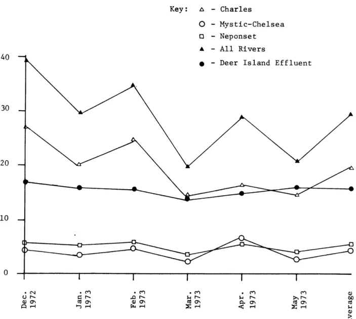
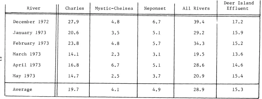
The river flow data was obrained from the United States Geological Survey (USGS) gauging stations located at Waltham for the Charles River, Norwood for the Neponset River and at Winchester for the Mystic and Chelsea Rivers. The correction factors to account for the river inflow in the ungauged areas below the gauging stations (USGS) are 1.2, 1.9 and 2.5 for the Charles, Neponset and Mystic-Chelsea Rivers respectively. The monthly averages are computed from the daily averages for the period from mid December 1972 to mid may 1973; the May average for the Mystic-Chelsea Rivers is estimated from the Charles River average by computing its average fraction of the Charles River flow. The monthly treated sewage effluent flows are from the Metropolitan District Commission Deer Island Treatment Plant monthly records of primary treatment (Table la), (Figure 2a). At high tide there is a large flow of salt water into the sewer system through improperly operating combined storm water and sewage tidal gates which are located mainly in the Boston Inner Harbor
(Figure 2) (Hydroscience, 1971). This unregulated flow can be up to 25% of the total treatment plant effluent. It is also heavily chlorinated to kill coliform bacteria.
Key: & - Charles
O - Mystic-Chelsea o - Neponset
A - All Rivers
40
-4 - Deer Island Effluent
30 I 20 10 oja' Co 4) r Cdo'N 0
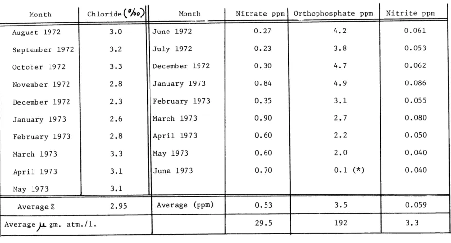
This addition of chlorine, without the other ions which constitute seawater, makes the actual determination of salinity nebulous at best, since it is in part based on an empirically
derived relation between various ions found in ocean water far from the coasts. The monthly average chlorinity (Table lb) of 2.95 0/oo corresponds to a salinity of 5.35 O/oo (Knudsen, 1962). This is considered very brackish water.
The major dissolved ions in river water are carbonate, sulfate and calcium, whereas chloride and sodium form only a minor
portion of the total dissolved matter (Neumann and Pierson, 1966). Therefore, the addition of large fluxes of unknown ions makes the determination of salinity from chlorinity with great accuracy not possible in the brackish waters found in Boston Harbor and parts of Massachusetts Bay. The use of electronic devices such as a Conductivity-Temperature-Depth sensor still presents the same problems; the relationship between conductivity and temperature and salinity is also empirically derived.
3.2 Estimate of Dissolved Nutrient Concentrations from Theory From the theoretical presentation, it should be possible to estimate the concentration of a dissolved nutrient in the harbor, given the exchange volumes and fluxes and a source flux. The
volume flux of E is taken as the mean monthly average of 15.3 cubic meters per second (Table la). Both the exchange flux Q and the sink
flushing number are functions of the half tidal cycle average velocity. Table 2 gives various combinations of the source flux E concentra-tions (Table lb has spot monthly values of the concentraconcentra-tions) and half tidal cycle average velocities, along with the resulting concentrations that would be present in the harbor. The depth d for the Q flux was assumed to be a constant three meters. Figure 5 is a plot of a non-dimensionalized C(I) versus Uo; the concentration is a function of Uo to the -i and -3/2 powers, and becomes especially high with a low Uo. Comparing these predicted
values of C(I) with the observed concentrations of different dissolved nutrients (Figures 21-24, 26, 33, 39, 48 and 49) it appears the observed values are of the same order of magnitude as what is predicted. However, more dissolved nutrient concentrations in the harbor and a better estimate for the depth of the mixed layer d are needed for a better statistical verification of C(I). The dissolved orthophosphate concentrations appear to be the best tag for the harbor water in the bay, mainly because of their high concentrations in the effluent flux.
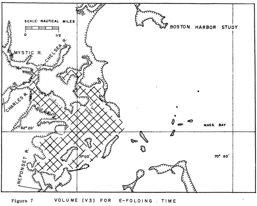
The e-folding time for dimensionalized exchange and harbor volume is given in Figure 6. The volume estimate for the harbor is from the Hydroscience report (1971), where the volume is taken for only the northern half of the harbor (Figure 7). The e-folding
-29-time varies from three to eleven tidal cycles for Boston Harbor, but that is assuming a constant half tidal cycle average velocity for all the tidal cycles. The actual e-folding time would be that derived from the mean half tidal cycle average velocity, about five tidal cycles.
3.3 Field Observations
3.3.1 Methods of Data Collection
The field investigation in the area of the mouth of Boston Harbor was undertaken with three main objectives: first, to determine the actual distribution of chemical nutrients from the area of the inner harbor out to Massachusetts Bay, second, to attempt to verify the flushing theory just presented and third, to determine if it is feasible to estimate the nutrient distribution (a time consuming chemical analysis) by correlation of the dissolved nutrient concentration with another variable that can be measured easier electrically, e.g., sigma-t.
Cruise 1 (August 16-17, 1972) was made for a background study. Work was attempted during the winter, but rough seas made small vessel data collection difficult. On Cruise 6
(March 15, 1973) the area coverage outside Boston Harbor was
more extensive, but no CTD casts were made, only surface temperature, salinity and nutrient samples were taken. Cruises 7, 8 and 9
covered essentially the same area, but included both CDT casts and nutrient samples; on Cruise 7 nutrient samples were taken at the surface, on Cruise 8 they were taken at one and one-half meters and on Cruise 9 they were taken at both the surface and
three and one-half meters.
All field work was carried out on the Massachusetts Institute of Technology RV R. R. Shrock, using CTDs built by the M.I.T. meteorology department. The temperature and pressure calibrations were done mechanically, the conductivity calibrations were done electrically. No attempt was made to take salinity bottle samples due to the brackish nature of the harbor and
effluent water. Thus, the salinity and sigma-t values obtained are only relative to each other and should not be considered as absolute values. The data was recorded in analog format on the ship, along with a reference clock signal. On shore it was transformed into a digital format on a Honeywell mini-computer. Final processing was accomplished on a PDP-7 computer to obtain station listings and temperature and salinity versus depth, sigma-t versus depth and temperature versus
salinity plots. The conversion of temperature, conductivity and pressure into salinity and sigma-t was done using a standard Woods Hole Oceanographic Institute computer subroutines (in use in 1972). Since the work was undertaken in shallow water the assumption was made that 1.0 decibar of pressure was
-31-equivalent to 1.0 meters of depth. For a pressure of 30 decibars, 30.0 db. = 29.77 m., the error would be only 0.9% (Neumann
and Pierson, 1966). The dissolved chemical nutrient concentrations were determined using a Technicon Autoanalyzer. The salinity of
the surface samples from Cruise 6 were determined with a Bissett-Berman benchtop salinometer.
3.3.2 Cruise 1
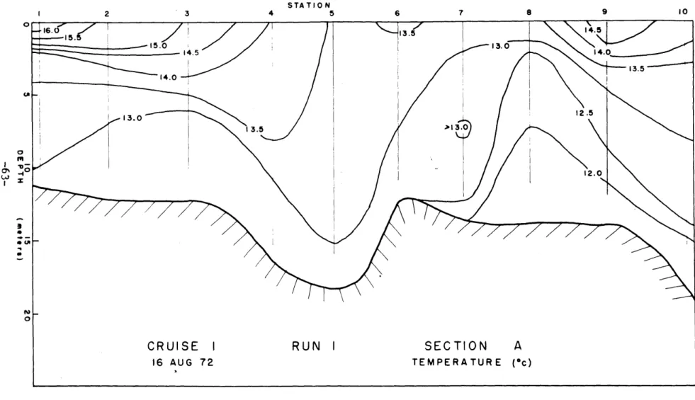
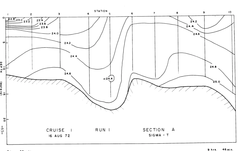
Cruise 1 was on August 16-17, 1972, and consisted of four runs from the inner harbor to outside the mouth of the harbor (Figure 8). The stations 5, 15, 25, 35 are located at the Deer Island Treatment Plant outfall.
On run 1 (Figures 9-11) the inversions and other small anomalies present are due to the brackish water; they are
shown on the sections to exhibit the data collected, some of the smaller ones have been removed. The anomalies are probably due to the methods of measurement. Seaward, at Station 9, the pool of warm, fresh and light water on the surface is probably
effluent from the previous ebb tide coming back on the present flood tide. The warm and fresh river water coming through the inner harbor has mixed with the water in President Roads and lost its distinguishing characteristics by Station 4. From Station 4 the Deer Island effluent presents itself as a new source of fresh, warm water.
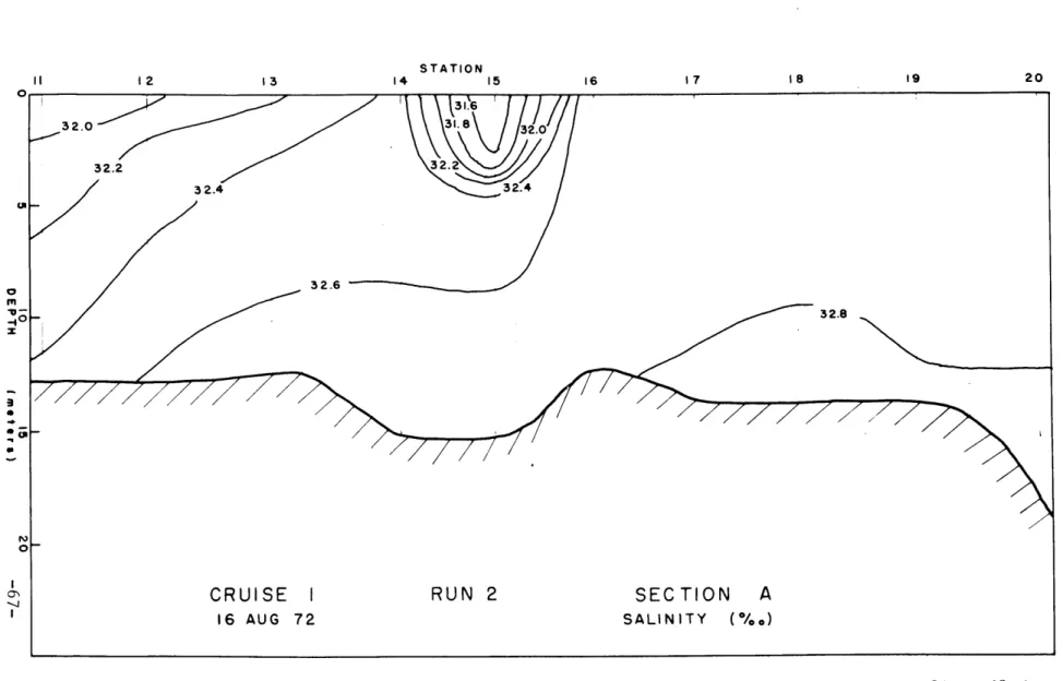
Run 2 (Figures 12-14) was made at high water. The main feature is the pool of warm, fresh water forming above the Deer Island outfall (Station 15).
The third run (Figures 15-17) was taken half way into the ebb tide. At Stations 25-27, the pool of fresh, warm water on the surface is part of the Deer Island effluent. Warm, fresh river water has moved from the inner harbor into President Roads, (Stations 21-24) but the Deer Island effluent still presents itself as a new water source at Station 25.
The final run (Figures 18-20) was at the end of the ebb tide, essentially low water. The light effluent water is present at Station 35, Deer Island, and also furter seaward as a pool centered at Station 37. The density inversion at Stations 38-39 is probably from the brackish nature of the water. The very warm pool (160C) is power plant cooling water, coming from
the southwest of Station 33. The Deer Island effluent is still separable as a new source of warm water.
To summarize the hydrographic stations from Cruise 1, Deer Island water is a source of warm, light and brackish water which rises to the surface, moves seaward with the ebb tide, where it mixes somewhat with the bay water, and then comes
back towards the harbor on the subsequent flood tide. The river inflow and the power plant cooling water are mixed with
the surrounding waters before Deer Island, thus the Deer Island
-33-Treatment Plant water is easily traced as a new source of high temperature and low salinity; low density water.
On the surface samples for this cruise, the nitrite concentrations were determined (Figures 21-24). Referring to what has been described in the vertical sections, the horizontal sections of the nitrite concentrations show the movement of the
effluent as a separate water mass. On run one, during the beginning of the flood tide, an area of high concentration outside the harbor is separated from the harbor by an area of low concentration. Going to slack water, run two, the concentration outside the harbor has decreased, while the levels inside the harbor itself have
remained essentially the same. On the ebb tidal flow during run three, the concentrations outside the harbor are building up, while the concentrations in the harbor, especially near the inner harbor, are also increasing. The increase of the concentrations
near the inner harbor is from the high levels of pollution in the inner harbor (Hydroscience, 1971, Environmental Protection Agency, 1971). At low water, run four, the concentrations both in the harbor and outside of it are uniformly ligh.
3.3.3 Use of only Sigma-t
Sigma-t will be used in the presentation of the remaining sections mainly for simplicity. As has been shown in the analysis of Cruise 1, the Deer Island effluent water is of very low salinity and is warmer than the surrounding waters, corresponding to a very
river inflow water. Thus, the Deer Island water can be traced by either temperature and salinity or by sigma-t alone.
3.3.4 Cruise 6
Cruise 6 (Figures 25-26) on March 15, 1973 was during the period from ebb tide to slack water. No CTD stations were made due to minor equipment problems, but surface samples were
taken for nitrite concentrations, salinity and temperature. The salinity and temperature were converted into sigma-t using Knutsen's Hydrographical Tables (1962). The effluent has gone to the northeast during this cruise, as can be noted from the curvature of the 24.0 isopycnal to the east and the high nitrite concentrations in the same area.
3.3.5 Cruise 7
Cruise 7 on April 19, 1973 was centered around slack water at high tide. The data is presented as longitudinal section B, transverse sections E, F and G, and surface nitrite plus nitrate concentrations (Figures 27-33).
In section B a strong outflow of the Deer Island effluent shows at Station3. The seasonal pycnocline is just beginning to develop, and it is at two and one-half to three meters depth, except at Station 7 where it rises to within a meter of the
surface. Section E has a core of light (26.4 sigma-t) Deer Island water which essentially disappears at Station F, but reappears further seaward on Section G. The 26.4 sigma-t water in section G
-35-is probably from the previous ebb tide, and -35-is separated from the landward 26.4 sigma-t water of the present ebb tide by denser water from the bay which mixed in during the flood tide.
The horizontal sections of the 1.0 meter sigma-t and surface nitrites plus nitrates also shows this apparent
separation of the ebb tidal flows. The seaward rise, fall and rise of the nutrient concentrations corresponds very well to the inverse fall, rise and fall of the sigma-t values.
3.3.6 Cruise 8
On Cruise 8, from high water to maximum ebb flow on May 3, 1973, the vertical sections F, G and H and the one and one-half meter orthophosphates represent the data collected
(Figures 34-39). The lack of data closer to the harbor makes it difficult to conclude much about the movement of the Deer Island effluent water. On section G a pool of 24.6 sigma-t water appears to be Deer Island effluent. The horizontal orthophosphate section
shows this water may be from the previous ebb tide, and is presently being dispersed. The center of the high orthophosphate concentra-tion water is landward of secconcentra-tion G.
On Section H, the furthest west of any section taken on any of the cruises, the pycnocline (at approximately 25.2 isopycnal) is at five meters depth. Assuming it has been present for an inertial period (14 hours, approximately at 42*N), below
3.3.7 Cruise 9
The last cruise, 9, on May 23, 1973 was centered around
high water. The data consists of longitudinal section B, transverse sections C, E, F and G, and surface and three and one-half meter orthophosphate horizontal sections (Figures 40-49).
Section B shows the release of Deer Island effluent between Stations 3 and 4. The pool of less than 24.6 sigma-t water below ten meters on these two stations is probably due to the
chemical composition of the water, and may not be real. The pycnocline rises from fifteen meters at the seaward end of
the section, Station 21, and then drops to meet the bay floor just outside the harbor at Station 5. The 24.6 sigma-t water
on sections C and E disappears by section F. The apparent inversion in section E, centered at Station 10, is again due to the
composition of the brackish Deer Island effluent water. On the seaward sections E, F and G the pycnocline (25.4 isopycnal) tilts upward to the southeast. Assuming this feature has existed for an inertial period, the geostrophic current
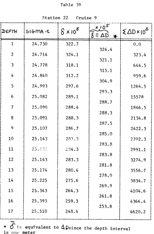
was calculated between Stations 21 and 22 on section G (Figure 45) (Tables 3a, 3b, 3c). (See Neumann and Pierson, 1966, for a detailed explanation of the calculation).
Fourteen meters was used as the reference level of no motion. Down to that level there is a current with a 2.6
centimeters per second maximum velocity away from the harbor.
-37-Below fourteen meters a current of up to 7.7 centimeters per second is moving in the opposite direction towards the harbor. Since and anomaly of the specific volume 6 was averaged over
one meter intervals, a slight possible error in the zeroing
of the depth measurements of up to a possible one-fourth meter would not have any significant effect on the net result of the
computations. A relative easterly geostrophic flow exists down to fourteen meters, and a stronger westerly flow is present below that level.
The orthophosphate sections indicate a pool of high
concentra-tion outside the harbor, along with very high concentraconcentra-tions in the harbor at President Roads. The pool of high concentration outside
the harbor may be from the previous ebb flow, while the high concentrations in President Roads is due to the release of Deer Island effluent during the present flood tide.
The three and one-half meter orthophosphate and the 1.0
meter sigma-t sections show a tongue of high phosphate, low sigma-t water moving out of the harbor, and also a pool of low phosphate-high sigma-t water centered about Station 9, section E. The 10.0 meter sigma-t section shows a rise of the isopycnal surfaces about the same area, implying the possibility of very light surface water; the isopycnal surfaces rising to maintain
the hydrostatic balance. Another possibility is the rising of the 10.0 meter isopycnal surfaces may be due to vortex type motion,
perhaps from the start up of the ebb tidal jet.
The faster moving light upper water creates a low pressure like area, allowing the dense lower water isopycnal surfaces to rise.
Section C has the interesting feature of "V" shaped isopycnals. Assuming an inertial period to set up, a current is flowing into the harbor along the southeastern edge of the harbor mouth, and a current is flowing out of the harbor along the northwestern edge. The inertial period required to set up a geostrophic current is about fourteen
hours and the tidal velocities through section C are up to one meter
per second; the shape of the isopycnals may be due to tidal action
alone. A geostrophic current of about ten centimeters per second would have only a small effect on the analysis of the tidal exchange
problem.
-39-The disappearance of the high orthophosphate water by section F corresponds to the loss of the 24.6 sigma-t water.
3.3.8 Aerial Observations
On Cruise 9 during the return into Boston Harbor (one and one-half hours into ebb tide) there was a visual sighting of a surface
slick which appeared to originate above the location of the outfall (Figure 50). A photograph taken at that time (Figure 51) shows the slick in the foreground, and the rougher water in the background, beginning at the Deer Island light. The rougher water (capillary waves present) had also just been passed through by the ship.
Subsequently, on May 26, 1973, photographs were taken of the Deer Island effluent plume from a commercial flight from Logan International Airport, Boston. One-half hour into ebb tide, the plume extends from inside the harbor entrance, on the right, to out-side the harbor (Figure 52). The next photograph (Figure 53) was taken a minute or so later, the wake of the freighter has stirred
water up from below the plume, showing it to be only a surface feature. 3.3.9 Wind Induced Surface Currents
Neumann and Pierson (1966) give an empirical formula for the surface drift currents induced by wind stress, derived by Thorade. The dependence of Vo, the induced current, on latitude is
Vo =2.59 w w < 6m/sec (approx.)
Vo =1.26w w > 6m/sec
where Vo is given in centimeters per second if w, the wind speed, is measured in meters per second. The mean wind and surface
currents (Table 4) are from Logan Airport, located north of President Roads. The twelve and twenty-four hour averages are for these
periods preceeding the last station of the cruises. The velocities from the RV R. R. Shrock are averaged from the half hourly readings taken during the cruises.
The surface currents, using the Logan data, averaged from 5.2 to 6.6 centimeters per second; a water parcel would
travel 1200 to 1500 meters during a 6.3 hour tidal period.
With a tidal excursion (R2) of ten thousand meters and an easterly or westerly wind, the variation in R2 would be approximately
ten percent. The effect is relatively small, but a knowledge of the recent and predicted winds would lead to a better ability
to predict the nutrient concentrations in the harbor. The derivation of the original theory was fairly crude, thus no
attempt was made to predict the minor effects of the wind induced surface currents.
-41-3.4 Dissolved Nutrient - Sigma-t Correlations
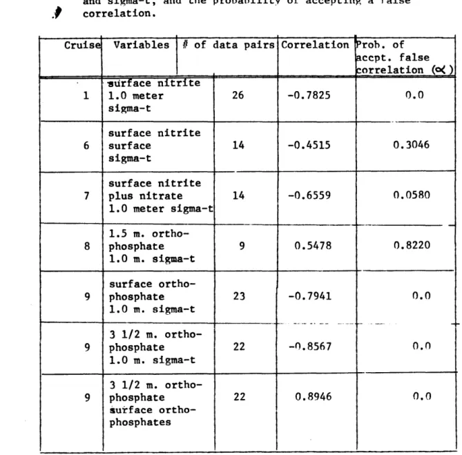
The dissolved nutrient concentrations and the one meter sigma-t values were correlated for cruises 1, 6, 7, 8 and 9. The correlations, number of data points measured and a, the
probability of accepting a false hypothesis, are listed in Table 5. The low level of significance for Cruise 8 is from the low number of data pairs (nine) and thus will not be discussed further. Cruises 1, 7, and 9 present high correlations with 95% levels of significance (5% a). Cruise 6, with a somewhat lower correlation, still has a 70% level of significance.
From this correlation data, and both the horizontal and vertical sections showing evidence of pools of high nutrient concentrations corresponding to pools of low sigma-t, there is a strong correspon-dence between dissolved nutrient concentrations and sigma-t values.
However, caution must be exercised before going out in the field and measuring the sigma-t values to conclude what the
nutrient concentrations are. Sigma-t values change significantly during the year due to the spring runoff into the bay, and the late fall overturning. A mapping of the surface sigma-t values would make it possible only to conclude the relative values of the nutrient concentrations. From these, it would be possible to identify and follow the Deer Island effluent water mass.
a least squares linear regression of concentration of dissolved orthophosphates on sigma-t was performed on the 1.0 meter
sigma-t data from Cruise 9 (Figure 54). The equation for concentration C from sigma-t is
C = 39.9259 - 1.5315 (sigma-t).
The regression orthophosphates do not define the Deer Island effluent as well as the observed concentrations, but the effluent is still evident.
-43-CHAPTER 4 RESULTS
4.1 Release of "Blobs"
If the surface chemical data from Cruise 1 is referred to (figs. 21-24), there is the movement of what appear to be "blobs" of harbor water seaward. Following is a schematic times series of what may be occurring.
At ebb tide, low water, a long tongue of harbor water protrudes into the bay.
Harbor 1
harbor water
Bay During the flood tide, the sink flow mixes harbor and bay water near the harbor, while the harbor water further seaward is cut off and remains essentially unmixed.
Harbor
harbor water
If
At slack water, high tide, the harbor water mass in the bay has moved landward, back towards the harbor.
Harbor
'T---]
II
r
\--.harbor water
BayAt the second ebb tide low water, a long tongue of harbor water is again protruding into the bay, and further seaward is a "blob" of harbor water from the previous ebb tide.
Harbor Bay
water harbor water from previous ebb tide
A rough estimate of the size of the homogenous harbor water mass, the "blob", is 2000 to 4000 meters long and 1500 meters wide. It is at present impossible to estimate the spacing of the "blobs" further out in the bay due to lack of sufficient data.
Edmonds (1973) has reported anomalies of dissolved nutrient concentrations in north-south sections in the region of sections G and H, Cruise 8 (fig. 34). These anomalies may be from "blobs"
of harbor water moving seaward.
-45-CHAPTER 5
SUMMARY AND CONCLUSIONS
A simple theoretical model for concentration in a harbor of a source flux at the harbor mouth was derived. Field observations consisting of five cruises were made in Boston
Harbor and adjacent Massachusetts Bay. One hundred stations were taken, most with both a CTD and nutrient bottle samples. Since the water being investigated was very brackish, no salinity bottle samples were taken to check the conductivity (salinity) calibrations of the CTD.
Wind induced surface and possible bottom geostrophic currents were calculated; they were found to be less than ten centimeters per second. The hydrographic data was summarized in vertical sections, the nutrient data in horizontal sections. A computation of C(I), the theoretical concentration of dissolved nutrients in
the harbor, was compared to the observed values. The conclusions, in no particular order, are:
1) From the theoretical derivation, the concentration of a flux source at the mouth of a basin-shaped harbor with strong tidal currents, and the sink flushing number determine the con-centration of that source in the harbor itself, independent of the volume of the harbor.
2) In Boston Harbor, with river and source fluxes of the same magnitude and separated spatially, the effluent source is a
3) The Deer Island effluent source, and possibly the harbor water move seaward as large homogenous water masses,
"blobs", one "blob" being emitted on each ebb tide. 4) An apparent geostrophic current of up to ten centimeters per second exists below the pycnocline in Massachusetts Bay, flowing towards the harbor at the time
of observation. From the conservation of salt mass, this water may mix with the above lying water by entrainment and vertical advection, subsequently flowing out to sea.
c~c~---5) From aerial observations, the effluent does not mix immediately with the harbor water flowing through the harbor mouth at Deer Island. The effluent is a distinct water mass which floats on the harbor and bay water, slowly mixing with them by diffusion. The theoretical derivation had assumed uniform and complete mixing of the harbor water and Deer Island effluent, especially in the harbor itself.
This report represents just a beginning of a study of the circulation between Boston Harbor and Massachusetts Bay, and a greater study of the circulation in the bay as a whole.
-47-Areas for further investigation started by this study are: 1) The movement of the harbor water and effluent as "blobs" seaward, and the diffusion of the "blobs" into the surrounding waters, possibly by aerial observation.
2) The effects of the geostrophic currents on the general circulation, possibly by a synoptic survey over several tidal periods. Along with this, a month long survey to determine the effects of the monthly tidal velocity variations.
3) Use of a hydroglider (Mollo-Christense, 1972) for rapid hydrographic coverage of a much expanded area of study.
4) A better calibration of the CTD, possibly with salinity bottle samples on each cast and a correction for brackish water.
5) The effects of storm surges on the nutrient concentrations in the harbor.
6) The possibility of vortices in the bay, formed by the start up of the ebb tidal jet.
7) A sink flow model which does not break down for 2b - R2, the jet excursion distance.
References
Aarons, Arnold B. & Henry Stommel, 1951, A Mixing Length Theory of Tidal Flushing, Trans. Amer. Geo. Union, 32, (3), pp. 419-21. Bendand, Julius S. & Allan G. Piersol, 1971, "Random Data:
Analysis and Measurment Procedures", John Wiley & Sons, Inc., New York.
Boating Almanac, 1972, Vol. 1, G. C. Bromley, & Co., New York. Bowden, K. F., 1967, in "Estuaries", George Lauff, ed., AAAS. DeFalco, Paul Jr., 1967, in "Estuaries", George Lauff, ed., AAAS. Edmonds, John, 1973, personal communication and unpublished data. Environmental Protection Agency (United States), 1971, Proceedings, Conference In the Matter of Pollution of the Navigable Waters
of Boston Harbor and its Tributaries - Massachusetts Third Session, October 27, 1971, Boston, Massachusetts.
Fischer, Hugo B., 1972, Mass Transport Mechanisms in Partially Stratified Estuaries, J.F.M., 53, (4), pp. 671-687.
Hydroscience, Inc., 1971, "Final Report, Development of Water Quality Model of Boston Harbor", prepared for Water Resources Commission, Commonwealth of Massachusetts.
Ketchum, Bostwick H., 1951, The Exchanges of Fresh and Salt Waters in Tidal Estuaries, J.M.R., X, (1), pp. 18-38.
Knudsen, Martin, 1962, "Hydrographical Tables", reprint, G. M. Manufacturing Company, New York.
Mollo-Christensen, Erik, 1972, personal communication. Neumann, Gerhard & Willard J. Pierson, 1966, "Principles of Physical Oceanography", Prentice Hall, Inc., New Jersry. Overland, James E,, 1972, A Review of Estuarine Modeling, Proceedings 18th annual Tech. Meet. Instit. of Environ. Sciences, pp. 178-185.
Pritchard, D. W., 1967, in "Estuaries", George Lauff, ed., AAAS.
-49-Rattray, Maurice Jr., & Donald V. Hansen, 1962, A Similarity
Solution for Circulation in an Estuary, J.M.R., 20, (2), pp. 121-133. Stommel, Henry, 1972, personal communication.
--- and H. G. Farmer, 1952, "On the Nature of Estuarine circulation", Part TI, Ref. No. 52-51, Woods Hole Oceanog. Instit. Taylor, G. I., 1960, "Selected Papers of G. T. Taylor", G. K. Batchelor, ed., pp. 172-184. (Orginally published 1921, Proc. London Math. Soc., Ser. 2, XIX, pp. 196-212.)
Table IA
Monthly Average River and Deer Island Effluent Flows
River Charles Mystic-Chelsea Neponset All River;
December 1972 27.9 4.8 6.7 39.4
January 1973 20.6 3.5 5.1 29.2
February 1973 23.8 4.8 5.7 34.3
March 1973 14.1 2.3 3.1 19.5
A... 1 1L7 7 I li 0 -7 r
Table
lB
Spot once-a-month Effluent Chemical Concentrations
Chloride(lo) Month Nitrate ppm Orthopho
I
~ ~
~
______________E . -- ________ August 1972 September 1972 October 1972 November 1972 December 1972 January 1973 February 1973 March 1973 April 1973 May 1973 3.0 3.2 3.3 2.8 2.3 2.6 2.8 3.3 3.1 3.1 June 1972 July 1972 December 1972 January 1973 February 1973 March 1973 April 1973 May 1973 June 1973 0.27 0.23 0.30 0.84 0.35 0.90 0.60 0.60 0.70 sphate ppm Nitrite ppm 4.2 3.8 4.7 4.9 3.1 2.7 2.2 2.0 0.1 (*) 0.061 0.053 0.062 0.086 0.055 0.080 0.050 0.040 0.040 Average% 2.95 Average (ppm) 0.53 3.5 0.059 AverageA. gm. atm./l. 29.5 192 3.3The chloride concentrations are true monthly averages. The other chemical concentrations Month
I - - I
Table 2
Predicted values of dissolved nutrient concentrations in Boston Harbor from theory. The tidal velocities are the maximum, mean, and minimum hftc. The values of E are from the average of the spot monthly values.
E Uo C(I)
,A gm. atm./l. meters per second g(gm. atm./l.
0.66 1.58 192 0.43 2.60 Orthophosphates 0.20 6.68 0.66 0.243 29.5 0.43 0.400 Nitrates 0.20 1.026 0.66 0.0269 3.3 0.43 0.0448 Nitrites 0.20 0.1146
-53-Table 3A
Station 21 Cruise 9
..
FTH
& nmA-
IOF
o
10b
a I - =-24.684 24.656 24.661 24.790 24.908 24.978 25.078 25.102 25.187 25.156 25.156 25.187 25,273 25.462 25.647 25.909 26.070 327.0 329.8 329.3 316.9 305.3 299.1 289.5 287.2 279.1 282.1 282.1 279.1 271.0 253.0 235.4 210.5 195.3 324.8 329.5 323.1 311.3 302.2 294.3 287.3 2P3.1 280.6 282.1 280.6 275.0 262.0 244.2 222.9 202.9 n.0 328.4 657.9 981.0 1292.1 1594.3 1888.6 2175.Q 2459.0 2739.6 3021.7 3302.3 3577.3 3839.3 4083.5 4306.4 4509.3 *
6
is eqivalent is one meterto A1since the depth interval
~---t-Table 3B Station 22
5IG-TmA -t
8 xI
xI0 "~L\t~(IO
8~L~b
* I 4 1nDx-S
1 2 3 4 5 6 7 8 9 10 11 12 13 14 15 16 17 24.730 24.714 24.778 24.840 24.993 25.082 25.090 25.091 25.107 25.143 25.143 25.174 25.225 25.343 25.393 25.510 I * is equivalent is one meterto 4Psince the depth interval
-55-Cruise 9 :)EPTH 322.7 324.1 318.1 312.2 297.6 289.1 288.4 288.3 286.7 283.3 2S4.3 283.3 280.4 275.6 264.3 259.3 248.4
--324.4 321.1 315.1 304.9 293.3 288.7 288.3 287.5 285.0 283.8 283.8 281.8 278.0 269.9 261.8 253.8 0.0 323.4 644.5 959.6 1264.5 15578 1846.5 2134.8 2422.3 2702.3 2991.1 3274.9 3556.7 3834.7 4104.6 4366.4 4620.2 -- "--~ITable 3C
Geostrophic current from field of mass between stations 21 and 22, Cruise 9.
r
SRe
(oi
IC
r
uurr
urrar*
nt+ - Sh
Wi-ih
rm. /ec.
cm5./sec..
Depth )Xio
xa 1 0.0 2 .5.0 3 13.4 4 21.4 5 27.6 6 36.5 7 42.1 8 41.1 9 26.7 10 32.3 11 30.6 12 27.4 13 20.6 14 4.6 15 -21.1 16 -60.0 17 -120.9Di tance between the = 420 20' North. stations is I 1655 meters, --0.0 0.3 0.8 1.3 1.7 2.3 2.6 2.5 1.6 2.0 1.9 1.7 1.3 0.3 -1.3 -3.7 -7.4 -0.3 0.0 0.5 1.0 1.4 2.0 2.3 2.2 1.3 1.7 1.6 1.4 1.0 0.0 -1.7 -4.0 -7.7
Table 4
Wind Induced Surface Currents
Cruise 6 Cruise 7 Cruise 8 Cruise 9
15 March 1973 19 April 1973 3 May 1973 23 May 1973
Wind Current Wind Current Wind Current Wind Current
12 hour 12 hour 12 hour 12 hour
3.2 mosec 5.7 cm/sec 2.7 m/sec 5.2 cm/sec 2.6 m/sec 5.1 cm/sec 4.2 m/sec 6.5 cm/sec
110 2200 1600 2300
24 hour 24 hour 24 hour 24 hour
2.7 m/sec 5.2 cm/sec 3.0 m/sec 5.5 cm/sec 2.8 m/sec 5.3 cm/sec 4.3 m/sec 6.6 cm/sec
1100 2200 1500 2600
RR Shrock RR Shrock RR Shrock
5.4 m/sec 7.3 cm/sec 2.7 m/sec 5.2 cm/sec 7.6 m/sec 111.6 cm/sec
= 420 20' The twelve and twenty-four mean winds are from Logan International Airport, Boston for that period of time preceeding the last station of the cruises. The mean winds from the RR Shrock are from half hourly readings during the cruises.
Table 5 Correlations between
and sigma-t, and the correlation.
dissolved nutrient concentrations probability of accepting a false
Cruise Variables # of data pairs Correlation Prob. of ccpt. false orrelation (co) surface nitrite 1 1.0 meter 26 -0.7825 0.0 sigma-t surface nitrite 6 surface 14 -0.4515 0.3046 sigma-t surface nitrite 7 plus nitrate 14 -0.6559 0.0580 1.0 meter sigma-t 1.5 m. ortho-8 phosphate 9 0.5478 0.8220 1.0 m. sigma-t surface ortho-9 phosphate 23 -0.7941 0.0 1.0 m. sigma-t 3 1/2 m. ortho-9 phosphate 22 -0.8567 0.0 1.0 m. sigma-t 3 1/2 m. ortho-9 phosphate 22 0.8946 0.0 surface ortho-phosphates
o=
0.20 m/sec
c( 1) = E ( I
Q
E
2 b Uod
2C(-I
-IU/2
S 2 c (1)'=
(U')
(I+ (U ) )
where
C()
= C(I)
2b
E
U'
= Uo
4be
-2 -UoS
0=
0.43m/sec
Uo=
0.66
m/sec
2 3 4 5 6 7non-dimensionalized Uo versus C(I)
V2 )
V2
S
2c(I)'
(
I+-1/ 2 2(b
t
)
(Uo-
)
Figure 5f
= 0.458 (
tV2V3
10
e.f.
V2
V2
6 3 owhere
V3= 215x
10
rn
8
64
(D0
SCALE! NAUTICAL MILES
BOSTON
do
VOLUME (V3) FOR E-FOLDING
HARBOR STU
MASS. BAY
70 50so'
wa
SCALE' NAUTICAL MILES
0 1/2
BOSTON HARBOR STUDY
CRUISE I 16-17 AUG 72 10 20 30 40
0
I
MASS. BAY 70 50' I2 3 13.0 STATION 5 8 9 10
CRUISE
I
16 AUG 72RUN
I
SECTION
TEMPERATURE 7hrs. 39 min.Figure 9 Times refer to hours after high waLtr, Boston. Scale: 1 cm. = 500 meters
vertical distortion 250:1
9 hrs. 46 min.
A
(c)
2 3 32.2 STATION 9 10 2.6 32.4 32.8
CRUISE
I
16 AUG 72RUN
I
SECTION
A
SALINI TY (%,) 3 0-ISTATION 2 3 U' o -0 I N 0
CRUISE
I
16 AUG 72RUN I
SECTION
SIGMA - T 9 hrs. 46 mi n. 7 hrs. 39 min.Figure 11 Times refer to hours after high water, Boston. Scale: 1 cm. = 500 meters vertical distortion 250:1
II 12 13 STATION 15 16 17 13.0 18 19 20
CRUISE
16 AUG 72RUN 2
SECTION
TEMPERATURE 10 hrs. 29 min. 0 hrs. 43 min.A
(c)
II 12 13 STATION 19 20 32.6 32.8
CRUISE
I
16 AUG 72RUN 2
SECTION
A
SALINITY (%o) 10 hrs. 29 min.Figure 13 Times refer to hours after high water, Boston. Scale: 1 cm. = 500 meters vertical distortion 250:1
12 13 19 20 24.8
CRUISE
I
16 AUG 72RUN 2
SECTION
SIGMA - T Ohrs. , 43 min.A
STATIONSTATION 21 22 23 24 25 26 27 28 15.5 15.0 14.5 13.5 I 3.( 14.0 1 3.5 13.0
CRUISE
I
RUN 3
SECTION
A
17 AUG 72 TEMPERATURE (c)
2 hrs. 40 min.
Figure 15 Times refer to hours after high water, Boston. Scale: 1 cm. = 500 meters vertical distortion 250:1
29 30
0
12.5
21 22 23 3