Graph integration of structured, semistructured and unstructured data for data journalism

HAL Id: hal-02904797

https://hal.inria.fr/hal-02904797v2

Submitted on 29 Oct 2020

HAL is a multi-disciplinary open access

archive for the deposit and dissemination of

sci-entific research documents, whether they are

pub-lished or not. The documents may come from

teaching and research institutions in France or

abroad, or from public or private research centers.

L’archive ouverte pluridisciplinaire HAL, est

destinée au dépôt et à la diffusion de documents

scientifiques de niveau recherche, publiés ou non,

émanant des établissements d’enseignement et de

recherche français ou étrangers, des laboratoires

publics ou privés.

Graph integration of structured, semistructured and

unstructured data for data journalism

Oana Balalau, Catarina Conceição, Helena Galhardas, Ioana Manolescu,

Tayeb Merabti, Jingmao You, Youssr Youssef

To cite this version:

Oana Balalau, Catarina Conceição, Helena Galhardas, Ioana Manolescu, Tayeb Merabti, et al.. Graph

integration of structured, semistructured and unstructured data for data journalism. 36ème

Con-férence sur la Gestion de Données – Principes, Technologies et Applications (informal publication

only), 2020. �hal-02904797v2�

unstructured data for data journalism

Oana Balalau

, Catarina Conceição

, Helena Galhardas

, Ioana Manolescu

,

Tayeb Merabti

, Jingmao You

, Youssr Youssef

1

Inria, Institut Polytechnique de Paris,

2

INESC-ID and IST, Univ. Lisboa, Portugal,

ABSTRACT

Nowadays, journalism is facilitated by the existence of large amounts of digital data sources, including many Open Data ones. Such data sources are extremely heterogeneous, ranging from highly struc-tured (relational databases), semi-strucstruc-tured ( JSON, XML, HTML), graphs (e.g., RDF), and text. Journalists (and other classes of users lacking advanced IT expertise, such as most non-governmental-organizations, or small public administrations) need to be able to make sense of such heterogeneous corpora, even if they lack the abil-ity to define and deploy custom extract-transform-load workflows. These are difficult to set up not only for arbitrary heterogeneous in-puts, but also given that users may want to add (or remove) datasets to (from) the corpus.

We describe a complete approach for integrating dynamic sets of heterogeneous data sources along the lines described above: the challenges we faced to make such graphs useful, allow their inte-gration to scale, and the solutions we proposed for these problems. Our approach is implemented within the ConnectionLens system; we validate it through a set of experiments.

1

INTRODUCTION

Data journalists often have to analyze and exploit datasets that they obtain from official organizations or their sources, extract from social media, or create themselves (typically Excel or Word-style). For instance, journalists from Le Monde newspaper want to re-trieveconnections between elected people at Assemblée Nationale and companies that have subsidiaries outside of France. Such a query can be answered currently at a high human effort cost, by inspecting e.g., a JSON list of Assemblée elected officials (available from Nos-Deputes.fr) and manually connecting the names with those found in a national registry of companies. This considerable effort may still miss connections that could be found if one added informa-tion about politicians’ and business people’s spouses, informainforma-tion sometimes available in public knowledge bases such as DBPedia, or journalists’ notes.

No single query language can be used on such heterogeneous data; instead, we study methods to query the corpus by specify-ing some keywords and askspecify-ing for all the connections that exist, in one or across several data sources, between these keywords. This line of work has emerged due to our collaboration with Le Monde’s fact-checking team1, within the ContentCheck collabora-tive research project2. With respect to the scientific literature, the problem of finding trees that connect nodes matching certain search keywords has been studied under the name ofkeyword search over

1

http://www.lemonde.fr/les-decodeurs/

2

https://team.inria.fr/cedar/contentcheck/

structured data, in particular for relational databases [28, 53], XML documents [25, 37], RDF graphs [17, 33]. However, most of these works assumed one single source of data, in which connections among nodes are clearly identified. When authors considered sev-eral data sources [36], they still assumed that one query answer comes from a single data source.

In contrast, the ConnectionLens [14] system (that we are devel-oping since 2018) answers keyword search queries over arbitrary combinations of datasets and heterogeneous data models, indepen-dently produced by actors unaware of each other’s existence. To achieve this goal, weintegrate a set of datasets into a unique graph, subject to the following requirements and constraints:

R1. Integral source preservation and provenance: in jour-nalistic work, it is crucial to be able to trace each node within the integrated graph back to the dataset from which it came. Source preservation is in line with the practice ofadequately sourcing information, an important tenet of quality journalism.

R2. Little to no effort required from users: journalists of-ten lack time and resources to set up IT tools or data pro-cessing pipelines. Even when they may have gained ac-quaintance with a tool supporting one or two data models (e.g., most relational databases provide some support for JSON data), handling other data models remains challeng-ing. Thus, the construction of the integrated graph needs to be as automatic as possible.

C1. Little-known entities: interesting journalistic datasets feature some extremely well-known entities (e.g., highly visible National Assembly deputees such as F. Ruffin, R. Fer-rand etc.) next to others of much smaller notoriety (e.g., the collaborators employed by the National Assembly to help organize each deputee’s work; or a company in which a deputee had worked). From a journalistic perspective, such lesser-known entities may play a crucial role in making interesting connections among nodes in the graph. C2. Controlled dataset ingestion: the level of confidence

in the data required for journalistic use excludes massive ingestion from uncontrolled data sources, e.g., through large-scale Web crawls.

C3. Language support: journalists are first and foremost concerned with the affairs surrounding them (at the local or national scale). This requires supporting dataset in the language(s) relevant for them - in our case, French. R3. Performance on “off-the-shelf” hardware: Our

algo-rithms’ complexity in the data size should be low, and overall performance is a concern; the tool should run on

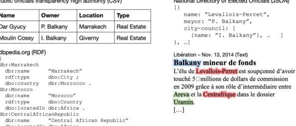
Figure 1: Motivating example: collection D of four datasets.

general-purpose hardware, available to non-expert users like the ones we consider.

To reach our graph-directed data integration goal under these requirements and constraints, we make the following contributions: (1) We define the novelintegration graphs we target, and for-malize the problem of constructing them from arbitrary sets of datasets.

(2) We introduce anapproach, and an architecture for building the graphs, leveraging data integration, information extrac-tion, knowledge bases, and data management techniques. Within this architecture, a significant part of our effort was invested in developing resources and tools for datasets in French. English is also supported, thanks to a (much) wider availability of linguistics resources.

(3) We have fully implemented our approach in an end-to-end tool; it currently supports text, CSV, JSON, XML, RDF, PDF datasets, and existing relational databases. We present: (𝑖 ) a set ofuse cases with real datasets inspired from our collab-oration with journalists; (𝑖𝑖 ) anexperimental evaluation of its scalability and the quality of the extracted graph. Motivating example. To illustrate our approach, we rely on a set of four datasets, shown in Figure 1. Starting from the top left, in clockwise order, we have: a table with assets of public officials, a JSON listing of France elected officials, an article from the newspa-per Libération with entities highlighted, and a subset of the DBPedia RDF knowledge base. Our goal is tointerconnect these datasets into a graph and to be able to answer, for example, the question: “What are the connections between Levallois-Perret and Africa?” One possible answer comes by noticing that P. Balkany was the mayor of Levallois-Perret (as stated in the JSON document), and he owned the “Dar Gyucy” villa in Marrakesh (as shown in the relational table), which is in Morocco, which is in Africa (stated by the DB-Pedia subset). Another interesting connection in this graph is that Levallois-Perret appears in the same sentence as the Centrafrican Republic in the Libération snippet at the bottom right, which (as stated in DBPedia) is in Africa.

2

OUTLINE AND ARCHITECTURE

We describe here the main principles of our approach, guided by the requirements and constraints stated above.

From requirement R1 (integral source preservation) it follows thatall the structure and content of each dataset is preserved in the in-tegration graph, thus every detail of any dataset is mapped to some of its nodes and edges. This requirement also leads us topreserve the provenance of each dataset, as well as the links that may exist within and across datasets before loading them (e.g. interconnected HTML pages, JSON tweets replying to one another, or RDF graphs referring to a shared resource). We termprimary nodes the nodes created in our graph strictly based on the input dataset and their provenance; we detail their creation in Section 3.

From requirement R2 (ideally no user input), it follows thatwe must identify the opportunities automatically to link (interconnect) nodes, even when they were not interconnected in their original dataset, and even when they come from different datasets. We achieve this at several levels:

• We leverage and extend information extraction techniques toextract (identify) entities occurring in the labels of every node in every input dataset. For instance, “Levallois-Perret” is identified as a Location in the two datasets at right in Figure 1 ( JSON and Text). Similarly, “P. Balkany”, “Balkany”, “I. Balkany” occurring in the relational, JSON and Text datasets are extracted as Person entities. Our method of entity extraction, in particular for the French language, is described in Section 4.

• We compare (match) occurrences of entities extracted from the datasets, in order to determine when they refer to the same entity and thus should be interconnected.

(1) Some entity occurrences we encounter refer to en-tities known in atrusted Knowledge Base (or KB, in short). For instance, Marrakech, Giverny etc. are de-scribed in DBPedia; journalists may trust these for such general, non-disputed entities. Wedisambiguate each entity occurrence, i.e., try to find the URI (identi-fier) assigned in the KB to the entity referred to in this

occurrence, and weconnect the occurrence to the en-tity. Disambiguation enables, for instance, to connect an occurrence of “Hollande” to the country, and two other “Hollande” occurrences to the former French president. In the latter case, occurrences (thus their datasets) are interconnected. We describe the module we built for entity disambiguation for the French lan-guage (lanlan-guage constraint C3), based on AIDA [27], in Section 5. It is of independent interest, as it can be used outside of our context.

(2) On little-known entities (constraint C1), disambigua-tion fails (no URI is found); this is the case, e.g., of “Moulin Cossy”, which is unknown in DBPedia. Com-bined with constraint C2 (strict control on ingested sources) it leads to the lack of reliable IDs for many entities mentioned in the datasets. We strive to con-nect them, as soon as the several identical or at least strongly similar occurrences are found in the same or different datasets. We describe our approach for comparing (matching) occurrences in order to identify identical or similar pairs in Section 6.

As the above description shows, our work recalls several known areas, most notably data integration, data cleaning, and knowledge base construction; we detail our positioning concerning these in Section 9.

3

PRIMARY GRAPH CONSTRUCTION FROM

HETEROGENEOUS DATASETS

We consider the followingdata models: relational (including SQL databases, CSV files etc.), RDF, JSON, XML, or HTML, and text. A dataset 𝐷𝑆 = (𝑑𝑏, 𝑝𝑟𝑜𝑣) in our context is a pair, whose first component is a concrete data object: a relational database, or an RDF graph, or a JSON, HTML, XML document, or a CSV, text, or PDF file. The second component 𝑝𝑟 𝑜 𝑣 denotes the dataset provenance; we consider here that the provenance is a URI, in particular a URL (public or private) from which the dataset was obtained. Users may not wish (or be unable to provide) such a provenance URI when registering a dataset; our approach does not require it, but exploits it when available, as we explain below.

Let 𝐴 be an alphabet of words. We define anintegrated graph 𝐺 = (𝑁 , 𝐸) where 𝑁 is the set of nodes and 𝐸 the set of edges. We have 𝐸 ⊆ 𝑁 × 𝑁 × 𝐴∗× [0, 1], where 𝐴∗denotes the set of (possibly empty) sequences of words, and the value in[0, 1] is the confidence, reflecting the probability that the relationship between two nodes holds. Each node 𝑛 ∈ 𝑁 has a label 𝜆(𝑛) ∈ 𝐴∗and similarly each edge 𝑒 has 𝜆(𝑒) ∈ 𝐴∗. We use 𝜖 to denote the empty label. We assign to each node and edge aunique ID, as well as a type (simple numbers, unique within one graph 𝐺). We introduce the supported node types as needed, and write them in bold font (e.g.,dataset node, URI node) when they are first mentioned; node types are important as they determine the quality and performance of matching (see Section 6). Finally, we create unique dataset IDs and associate to each node its dataset’s ID.

Let 𝐷𝑆𝑖 = (𝑑𝑏𝑖, 𝑝𝑟 𝑜 𝑣𝑖) be a dataset of any of the above models.

The following two steps are taken regardless of 𝑑𝑏𝑖’s data model:

First, we introduce adataset node 𝑛_{𝐷 𝑆}

𝑖 ∈ 𝑁 , which models the

dataset itself (not its content). Second, if 𝑝𝑟 𝑜 𝑣𝑖is not null, we create

anURI node 𝑛_{𝑝𝑟 𝑜 𝑣}

𝑖 ∈ 𝑁 , whose value is the provenance URI 𝑝𝑟𝑜𝑣𝑖

, and an edge 𝑛_{𝐷 𝑆}

𝑖

cl:prov

−−−−−→ 𝑛𝑝𝑟 𝑜 𝑣𝑖

, where cl:prov is a special edge label denoting provenance (we do not show these edges in the Figure to avoid clutter).

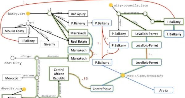
Next, Section 3.1 explains how each type of dataset yields nodes and edges in 𝐺 . For illustration, Figure 2 shows the integrated graph resulting from the datasets in Figure 1. In Section 3.2, we describe a set of techniques that improve the informativeness and the connectedness and decrease the size of 𝐺 . Finally, in Section 3.3, we give the complexity of constructing an integrated graph.

3.1

Mapping each dataset to the graph

A common feature of all the edges whose creation is described in this section is that we consider them certain (confidence of 1.0), given that they reflect the structure of the input datasets, which we assume trusted. Lower-confidence edges will be due to extraction (Section 4 and Section 5) and node similarity (Section 6).

Relational. Let 𝑑𝑏 = 𝑅 (𝑎1, . . . , 𝑎𝑚) be a relation (table) (residing

within an RDBMS, or ingested from a CSV file etc.) Atable node 𝑛_𝑅is created to represent 𝑅 (yellow node with labelhatvp.csv on top left in Figure 2). Let 𝑡 ∈ 𝑅 be a tuple of the form (𝑣1, . . . , 𝑣𝑚)

in 𝑅. Atuple node 𝑛𝑡is created for 𝑡 , with an empty label, e.g., 𝑡1

and 𝑡₂in Figure 2. For each non-null attribute 𝑣_𝑖in 𝑡 , avalue node 𝑛𝑣𝑖 is created, together with an edge from 𝑛𝑡to 𝑛𝑣𝑖, labeled 𝑎𝑖 (for

example, the edge labeledowner at the top left in Figure 2). To keep the graph readable, confidence values of 1 are not shown. Moreover, for any two relations 𝑅, 𝑅0for which we know that attribute 𝑎 in 𝑅 is a foreign key referencing 𝑏 in 𝑅0, and for any tuples 𝑡∈ 𝑅, 𝑡0∈ 𝑅0 such that 𝑡 .𝑎= 𝑡0.𝑏 , the graph comprises an edge from 𝑛𝑡 to 𝑛𝑡0

with confidence 1. This graph modeling of relational data has been used for keyword search in relational databases [28].

RDF. The mapping from an RDF graph to our graph is the most natural. Each node in the RDF graph becomes, respectively, a URI node or a value node in 𝐺 , and each RDF triple(𝑠, 𝑝, 𝑜) becomes an edge in 𝐸 whose label is 𝑝 . At the bottom left in Figure 2 appear some edges resulting from our DBPedia snippet.

Text. We model a text document very simply, as a node having a sequence of children, where each child is a segment of the text. Currently, each segment is a phrase; we found this a convenient granularity for users inspecting the graph. Any other segmentation could be used instead.

JSON. As customary, we view a JSON document as a tree, with nodes that are eithermap nodes, array nodes or value nodes. We map each node into a node of our graph and create an edge for each parent-child relation. Map and array nodes have the empty label 𝜖 . Attribute names within a map become edge labels in our graph. Figure 2 at the top right shows how a JSON document’s nodes and edges are ingested in our graph.

XML. The ingestion of an XML document is very similar to that of JSON ones. XML nodes are eitherelement, or attribute, or values nodes. As customary when modeling XML, value nodes are either text children of elements or values of their attributes.

HTML. An HTML document is treated very similarly to an XML one. In particular, when an HTML document contains a hyperlink of the form_{<a href=”http://a.org”>label</a>}, we create a node labeled “a” and another labeled “http://a.org”, and connect them through an

Figure 2: Integrated graph corresponding to the datasets of Figure 1. An answer to the keyword query {“I. Balkany”, Africa, Estate} is highlighted in light green; the three keyword matches in this answer are shown in bold.

edge labeled “href ”; this is the common treatment of element and attribute nodes. However, we detect that a child node satisfies a URI syntax, andrecognize (convert) it into a URI node. This enables us to preserve links across HTML documents ingested together in the same graph, with the help of node comparisons (see Section 6). Bidimensional tables. Tables such as one finds in spreadsheets, which we call bidimensional tables (or 2d tables, in short) differ in important ways from relational database tables. First, unlike a relational table, a 2d table featuresheaders for both the lines and the columns. As spreadsheet users know, this leads to certain flexibility when authoring a spreadsheet, as one feels there is not much differ-ence between a 2d table and its transposed version (where each line becomes a column and vice versa). Second,headers may be nested, e.g., the 1st column may be labeled “Paris”, the 2nd column may be labeled “Essonne”, and a common (merged) cell above them may be labeled “Ile de France”, as shown in Figure 3.

Figure 3: Conversion of a 2d table in a graph. To carry in our graph all the information from a 2d table, and enable meaningful search results, we adopt the approach in [12]

for transforming 2d tables into Linked Open Data (RDF). Specif-ically, we create aheader cell node for each header cell, shown as gray boxes at the bottom of Figure 3, and a value node for each data cell (white boxes in the figure). Further, each header cell node is connected through an edge to its ancestor header cell, e.g., the edge from the “Paris” node to the “Île-de-France” node. The edge has a dedicated label cl:parentHeaderCell (not shown in the figure), and each value cell node has edges going to its near-est header cells, edges labeled respectively cl:closnear-estXHeaderCell and cl:closestYHeaderCell. This modeling makes it easy to find, e.g., how Fred is connected to Île-de-France (through Essonne). In keeping with [12], we create a (unique) URI for each data and cell node, attach their value as a property of the nodes, and encode all the edges as RDF triples. The approach easily generalizes to higher-dimensional tables.

PDF. A trove of useful data is found in the PDF format. Many interesting PDF documents containbidimensional tables. We thus use a dedicated 2d table extractor: the Python Camelot library3, amongst the best open source libraries. We then generate from the 2d table a graph representation, as explained above. The tables are removed cell by cell from the PDF text, and lines of text are grouped with a rule-based sentence boundary detector so that coherent units are not split. In addition, we add a simple similarity metric to determine the horizontal and vertical headers. Final text content is saved in JSON, parents being the number of the line, children their content. Thus, from a PDF file, we obtain one or more datasets: (𝑖 ) at least a JSON file with its main text content, and (𝑖𝑖 ) as many RDF graphs as there were 2d tables recognized within the PDF. From the dataset node of each such dataset 𝑑𝑖, we add an edge

labeled cl:extractedFromPDF, whose value is the URI of the PDF file. Thus, the PDF-derived datasets are all interconnected, and trace back to their original file.

3

3.2

Refinements and optimizations

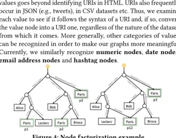
Value node typing. The need to recognize particular types of values goes beyond identifying URIs in HTML. URIs also frequently occur in JSON (e.g., tweets), in CSV datasets etc. Thus, we examine each value to see if it follows the syntax of a URI and, if so, convert the value node into a URI one, regardless of the nature of the dataset from which it comes. More generally, other categories of values can be recognized in order to make our graphs more meaningful. Currently, we similarly recognizenumeric nodes, date nodes, email address nodes and hashtag nodes.

Figure 4: Node factorization example.

Node factorization. The graph resulting from the ingestion of a JSON, XML, or HTML document, or one relational table, is a tree; any value (leaf ) node is reachable by a finite set of label paths from the dataset node. For instance, in the tree at left in Figure 4, two value nodes labeled “Paris” (indicated as 𝑝1, 𝑝2) are reachable on the

paths employee.address.city, while 𝑝3is on the path

headquarter-sCity (𝑝3). Graph creation as described in Section 3.1 creates three

value nodes labeled “Paris”; we call thisper-occurrence value node creation. Instead, per-path creation leads to the graph at right, where a single node 𝑝12is created for all occurrences of “Paris”

on the path employee.address.city. We have also experimented with per-dataset value node creation, which in the above example cre-ates a single “Paris” node, and withper-graph, where a single “Paris” value node is created in a graph, regardless of how many

times “Paris” appears across all the datasets. Note that:

(1) Factorization leads to a DAG (rather than a tree) represen-tation of a tree-structured document; it reduces the number of nodes while preserving the number of edges.

(2) The strongest form of factorization (per-graph) is consistent with the RDF data model, where a given literal leads to exactly one node.

(3) Factorization leads to more connections between nodes. For instance, at right in Figure 4, Alice and Bob are connected not only through the company where they both work, but also through the city where they live.

(4) Applied blindly on pure structural criteria, factorization may introduce erroneous connections. For instance, con-stants such astrue and false appear in many contexts, yet this should not lead to connecting all nodes having an at-tribute whose value istrue. Another example are named entities, which should be first disambiguated.

To prevent such erroneous connections, we have heuristically identified a set ofvalues which should not be factorized even withper-path, per-dataset or per-graph value node creation. Beyond true and false and named entities, this currently includes integer numeric node labels written on less than 4 digits, the rationale being that small integers tend to be used for ordinals, while numbers on

many digits could denote years, product codes, or other forms of identifiers. This very simple heuristic could be refined.

Another set of values that should not be factorized arenull codes, or strings used to signal missing values, which we encoun-tered in many datasets, e.g., “N/A”, “Unknown” etc. As is well-known from database theory, nulls should not lead to joins (or connections, in our case). We found many different null codes in real-life datasets we considered. We have manually established a small list; we also show to the userthe most frequent values en-countered in a graph (null codes are often among them) and allow her to decide among our list and the frequent values, which to use as null codes. The decision is important because these values will never lead to connections in the graph (they are not factorized, and they are not compared for similarity (see Section 6). This is why we consider that this task requires user input.

Factorization trade-offs are as follows. Factorization densifies the connections in the graph. Fewer nodes also reduce the number of comparisons needed to establish similarity links; this is useful since the comparisons cost is in the worst-case quadratic in the number of nodes. At the same time, factorization may introduce erroneous links, as discussed above. Given that we make no assumption on our datasets, there is no “perfect” method to decide when to factorize. The problem bears some connections, but also differences, with entity matching and key finding; we discuss this in Section 9.

As a pragmatic solution: (𝑖 ) when loading RDF graphs, in which each URI and each literal corresponds to a distinct node, we apply aper-graph node creation policy, i.e., the graph contains overall a single node for each URI/literal label found in the input datasets; (𝑖𝑖 ) in all the other datasets, which exhibit a hierarchical structure ( JSON, XML, HTML, a relational table or CSV file, a text document) we apply theper-dataset policy, considering that within a dataset, one constant is typically used to denote only one thing.

3.3

Complexity of the graph construction

Summing up the above processing stages, the time to ingest a set of datasets in a ConnectionLens graph 𝐺= (𝑁 , 𝐸) is of the form:

𝑐1· |𝐸 | + 𝑐2· |𝑁 | + 𝑐3· |𝑁𝑒| + 𝑐4· |𝑁 | 2

In the above, the constant factors are explicitly present (i.e., not wrapped in an 𝑂(. . .) notation) as the differences between them are high enough to significantly impact the overall construction time (see Section 8.4 and 8.5). Specifically: 𝑐₁reflects the (negligible) cost of creating each edge using the respective data parser, and the (much higher) cost of storing it; 𝑐₂reflects the cost to store a node in the database, and to invoke the entity extractor on its label, if it is not 𝜖 ; 𝑁_𝑒is the number of entity nodes found in the graph, and 𝑐3is the cost to disambiguate each entity; finally, the last

component reflects the worst-case complexity of node matching, which may be quadratic in the number of nodes compared. The constant 𝑐4reflects the cost of recording on disk that the two nodes

are equivalent (one query and one update) or similar (one update). Observe that while 𝐸 is entirely determined by the data, the number of value nodes (thus 𝑁 , thus the last three components of the cist) is impacted by the node creation policy; 𝑁𝑒(and, as we

4

NAMED-ENTITY RECOGNITION

After discussing how to reflect thestructure and content of datasets into a graph, we now look into increasing theirmeaning, by lever-aging Machine Learning (ML) tools for Information Extraction.

Named entities (NEs) [42] are words or phrases which, together, designate certain real-world entities. Named entities include com-mon concepts such as people, organizations, and locations. How-ever, the term can also be applied to more specialized entities such as proteins and genes in the biomedical domain, or dates and quan-tities. TheNamed-Entity Recognition (NER) task consists of (𝑖) iden-tifying NEs in a natural language text, and (𝑖𝑖 ) classifying them according to a pre-defined set of NE types. NER can be modeled as a sequence labeling task, that receives as input a sequence of words and returns a sequence of triples (NE span, i.e., the words referring together to the entity, NE type, 𝑐 ) as output, where 𝑐 is theconfidence of the extraction (a constant between 0 and 1).

Let 𝑛_𝑡be a text node. We feed 𝑛_𝑡as input to a NER module and create, for each entity occurrence 𝐸 in 𝑛𝑡, anentity occurrence

node (or entity node, in short) 𝑛𝐸; as explained below, we extract

Person, Organization and Location entity nodes. Further, we add an edge from 𝑛𝑡to 𝑛𝐸whose label is cl:extract𝑇 , where 𝑇 is the

type of 𝐸 , and whose confidence is 𝑐 . In Figure 2, the blue, round-corner rectanglesCentrafrique, Areva, P. Balkany, Levallois-Perret correspond to the entities recognized from the text document, while theMarrakech entity is extracted from the identical-label value node originating from the CSV file.

Named-Entity Recognition We describe here the NER approach we devised for our framework, for English and French. While we have used Stanford NER [18] in [14, 15], we have subsequently developed a more performant module based on the Flair NLP frame-work [1]. Flair allowstraining sequence labeling models using deep-learning techniques. Flair and similar frameworks rely on embed-ding words into vectors in a multi-dimensional space. Traditional word embeddings, e.g., Word2Vec [41], Glove [45] and fastText [8], arestatic, meaning that a word’s representation does not depend on the context where it occurs. New embedding techniques are dy-namic, in the sense that the word’s representation also depends on its context. In particular, the Flair dynamic embeddings [2] achieve state-of-the-art NER performance. The latest Flair architecture [1] facilitatescombining different types of word embeddings, as a better performance might be achieved by combining dynamic with static word embeddings.

The English model currently used in ConnectionLens is a pre-trained model4. It is trained using the English CoNLL-20035dataset which contains persons, organizations, locations, and miscella-neous (not considered in ConnectionLens) named-entities. The dataset consists of news articles. The model combines Glove em-beddings [45] and so-calledforward and backward pooled Flair em-beddings, that evolve across subsequent extractions.

To obtain a high-quality model for French, we trained our model on WikiNER [43], a multilingual NER dataset automatically created using the text and structure of Wikipedia. The dataset contains 132K sentences, 3.4M tokens and 216K named-entities, including 74K

4

https://github.com/flairNLP/flair

5

https://www.clips.uantwerpen.be/conll2003/ner/

Person, 116K Location and 25K Organization entities. The model uses stacked forward and backward French Flair embeddings with French fastText [8] embeddings.

Entity node creation. Similarly to the discussion about value node factorization (Section 3.2), we have the choice of creating an entity node 𝑛𝐸of type 𝑡 once per occurrence, or (in hierarchical

datasets)per-path, per-dataset or per-graph. We adopt the per graph method, with the mention that we will create one entity node for each disambiguated entity and one entity node for each non-disambiguated entity.

5

ENTITY DISAMBIGUATION

An entity node 𝑛_𝑒extracted from a dataset as an entity of type 𝑇 may correspond to an entity (resource) described in a trusted knowledge base (KB) such as DBPedia or Yago. As stated in Section 2, this is not always the case, i.e., we encounter entities that are not covered by KBs. However, when they are, the information is valuable as it allows: (𝑖 ) resolvingambiguity to make a more confident decision about the entity, e.g., whether the entity node “Hollande” refers to the former president or to the country; (𝑖𝑖 ) tacklingname variations, e.g., two Organization entities labeled “Paris Saint-Germain Football Club” and “PSG” are linked to the same KB identifier, and (𝑖𝑖𝑖 ) if this is desired,enriching the dataset with a certain number of facts the KB provides about the entity.

Named entity disambiguation (NED, in short, also known as en-tity linking) is the process of assigning a unique identifier (typically, a URI from a KB) to each named-entity present in a text. We built our NED module based onAIDA [27], part of the Ambiverse6 framework; AIDA maps entities to resources in YAGO 3 [38] and Wikidata [52]. Our work consisted of (𝑖 ) adding support for French (not present in Ambiverse), and (𝑖𝑖 ) integrating our own NER mod-ule (Section 4) within the Ambiverse framework.

For the first task, in collaboration with the maintainers of Am-biverse7, we built a new dataset for French, containing the infor-mation required for AIDA. The dataset consists of entity URIs, information about entity popularity (derived from the frequency of entity names in link anchor texts within Wikipedia), and entity context (a set of weighted words or phrases that co-occur with the entity), among others. This information is language-dependent and was computed from the French Wikipedia.

For what concerns the second task, Ambiverse takes an input text and passes it through a text processing pipeline consisting oftokenization (separating words), part-of-speech (POS) tagging, which identifies nouns, verbs, etc., NER, and finally NED. Text and annotations are stored and processed in Ambiverse using the UIMA standard8. A central UIMA concept is theCommon Annotation Scheme (or CAS); in short, it encapsulates the document analyzed, together with all the annotations concerning it, e.g., token offsets, tokens types, etc. In each Ambiverse module, the CAS object con-taining the document receives new annotations, which are used by the next module. For example, in the tokenization module, the CAS initially contains only the original text; after tokenization, the CAS also contains token offsets.

6

https://www.mpi- inf.mpg.de/departments/databases- and- information- systems/ research/ambiverse- nlu/

7

https://github.com/ambiverse- nlu/ambiverse- nlu#maintainers- and- contributors

8

To integrate our Flair-based extractor (Section 4), we deployed a new Ambiverse processing pipeline, to which we pass as input both the input text and the extracted entities.

Due to its reliance on sizeable linguistic resources, the NED mod-ule requires 93G on disk and 32G of RAM to support disambiguation for English (provided by the authors) and French (which we built). Therefore, we deployed it outside of the ConnectionLens code as a Web service, accessible in our server.

6

NODE MATCHING

This section presents our fourth and last method foridentifying and materializing connections among nodes from the same or different datasets of the graph. Recall that (𝑖 )value nodes with identical labels can be fused (factorized) (Section 3.2); (𝑖𝑖) nodes be-come connected asparents of a common extracted entity (Section 4); (𝑖𝑖𝑖 ) entity nodes with different labels can be interconnectedthrough a common reference entity when NED returns the same KB entity (Section 5). We still need to be able to connect:

• entity nodes with value nodes, in the case, when extrac-tion did not find anything in the value node. Recall that extraction also uses a context, and it may fail to detect entities on some values where context is lacking. If the labels are identical or very similar, these could refer to the same thing;

• entity nodes, such that disambiguation returned no result for one or both. Disambiguation is also context-dependent; thus, it may work in some cases and not in others; entity nodes with identical or strongly similar labels, from the same or different datasets, could refer to the same thing. • value nodes, even when no entity was detected. This

con-cerns data-oriented values, such as numbers and dates, as well as text values. The latter allows us to connect, e.g., ar-ticles or social media posts when their topics (short strings) and/or body (long string) are very similar.

When a comparison finds two nodes withvery similar labels, we create an edge labeled cl:sameAs, whose confidence is the similarity between the two labels. In Figure 2, a dotted red edge (part of the subtree highlighted in green) with confidence .85 connects the “Central African Republic” RDF literal node with the “Centrafrique”

Location entity extracted from the text.

When a comparison finds two nodes with identical labels, one could consider unifying them, but this raises some modeling issues, e.g., when a value node from a dataset 𝑑1is unified with an entity

encountered in another dataset. Instead, weconceptually connect the nodes with sameAs edges whose confidence is 1.0. These edges are drawn in solid red lines in Figure 2. Nodes connected by a 1.0 sameAs edge are also termedequivalent. Note that 𝑘 equivalent nodes lead to 𝑘(𝑘 − 1)/2 edges. Therefore, these conceptual edges are not stored; instead, the information about 𝑘 equivalent nodes is stored using 𝑂(𝑘) space, as we explain in Section 7.

Inspired by the data cleaning literature, our approach for match-ing isset-at-a-time. More precisely, we form node group pairs (𝐺𝑟1, 𝐺 𝑟2), and we compare each group pair using the similarity

function known to give the best results (in terms of matching qual-ity) for those groups. The Jaro measure [31] gives good results for short strings [16] and is applied to compute the similarity between pairs of entities of the same type recognized by the entity extractor

(i.e., person names, locations and organization names which are typically described by short strings). The common edit distance (or Levenshtein distance) [35] is applied to relatively short strings that have not been identified by the entity extractor. Finally, the Jac-card coefficient [30] gives good results for comparing long strings that have words in common and is therefore used to compute the similarity between long strings.

Table 1 describes our matching strategy. For each group 𝐺𝑟₁that we identify, a line in the table shows: a pair(𝐺𝑟1, 𝐺 𝑟2) as a logical

formula over the node pairs; the similarity function selected for this case; and the similarity threshold 𝑡 above which we consider that two nodes are similar enough, and should be connected by a sameAs edge. We set these thresholds experimentally as we found they lead to appropriate similar pair selections, in a corpus built from news articles from Le Monde and Mediapart, social media (tweets), and open ( JSON) data from nosdeputes.fr.

For Person, Location, and Organization, the similarity is com-puted based on normalized versions of their labels, e.g., for Person entities, we distinguish the first name and the last name (when both are present) and compute the normalized label as “Firstname Lastname”. For URI, hashcode, and email entities, we require iden-tical labels; these can only be found equivalent (i.e., we are not interested in a similarity lower than 1.0). Finally, we identifyshort strings (shorter than 128 characters) and long strings (of at least 32 characters) and use different similarity functions for each, given that the distinction is fuzzy, we allowed these categories to overlap. We explain how groups and comparison pairs are formed in Section 7 when describing our concrete implementation.

7

GRAPH STORAGE

The storage module of our platform consists of a Graph interface providing the data access operations needed in order to access the graph, and (currently) of a single implementation based on a relational database, which is accessed through JDBC, and which implements these operations through a mix of Java code and SQL queries. This solution has the advantage of relying on a standard ( JDBC) backed by mature, efficient and free tools, such as Postgres, which journalists were already familiar with, and which runs on a variety of platforms (requirement R3 from Section 1).

The tableNodes(id, label, type, datasource, label, normaL-abel, representative) stores the basic attributes of a node, the ID of its data source, its normalized label, and the ID of its represen-tative. For nodes not equivalent to any other, the representative is the ID of the node itself. As explained previously, the representa-tive attribute allows encoding information about equivalent nodes. TableEdges(id, source, target, label, datasource, confidence) stores the graph edges derived from the data sources, as well as the extraction edges connecting entity nodes with the parent(s) from which they have been extracted. Finally, theSimilar(source, tar-get, similarity) table stores a tuple for each similarity comparison whose result is above the threshold (Table 1) but less than 1.0. The pairs of nodes to be compared for similarity are retrieved by means of SQL queries, one for each line in the table.

This implementation requires an SQL query (through JDBC) to access each node or edge within the storage. As such access is ex-pensive, we deploy our own memory buffer: graph nodes and edges arefirst created in memory, and spilled to disk in batch fashion

Node group 𝐺𝑟1 Node pairs from(𝐺𝑟1× 𝐺𝑟2) to compare Similarity function Threshold

Person entity Person× Person Jaro 0.8 Location entity Location× Location Jaro 0.8 Organization entity Organization× Organization Jaro 0.95 URI, hashtag, or email Same label∧ same type Equality 1.0 Number Same label value∧ isNumber Equality 1.0 Date Same timestamp value∧ isDate Equality 1.0 Non-entity short string abs. len. < 128∧ rel. len. ± 20% ∧ prefix(3) match Levenshtein 0.8 Non-entity long string abs. len. > 32∧ rel. len. ± 20% ∧ has common word Jaccard 0.8

Table 1: Node matching: selectors, similarity functions, and thresholds. when the buffer’s maximum size is reached. Value node

factoriza-tion (Secfactoriza-tion 3.2) may still require querying stored graph to check the presence of a previously encountered label. To speed this up, we also deployed a memory cache of nodes by their labels forper-graph factorization, respectively, by (label, dataset, path) forper-path fac-torization etc. These caches’ size determines a compromise between execution time and memory needs during graph construction.

Other storage back-ends could be integrated easily as imple-mentations of the Graph interface; we have started experimenting with the BerkeleyDB key-value store, which has the advantage of running as a Java library, without the overhead of a many-tiers architecture such as JDBC.

8

PERFORMANCE EVALUATION

We now present results of our experiments measuring the perfor-mance and the quality of our various modules involved in graph construction. Section 8.1 presents our settings, then we present experiments focusing on: metrics related to graph construction in Section 8.2, the quality of our extraction of tables from PDF docu-ments in Section 8.3, of our information extraction in Section 8.4, finally of our disambiguation module in Section 8.5.

8.1

Settings

TheConnectionLens prototype consists of 46K lines of Java code and 4.6K lines of Python, implementing the module which extracts information from PDF (Section 3) and the Flair extractor (Section 4). The latter two have been integrated as (local) Web services. The disambiguator (Section 5) is Java Web service running on a ded-icated Inria server, adapting the original Ambiverse code to our new pipeline; the code has 842 classes, out of which we modified 10. ConnectionLens is available online athttps://gitlab.inria.fr/ cedar/connectionlens. We relied on Postgres 9.6.5 to store our integrated graph. Experiments ran on aserver with 2.7 GHz Intel Core i7 processors and 160 GB of RAM, running CentOs Linux 7.5. Data sources We used a set of diverse real-world datasets, de-scribed below from the smaller to the larger. Given that they are of different data models, we order them by theirsize on disk before being input in ConnectioneLens.

1. We built a corpus of 464 HTML articles crawled from the French online newspaper Mediapart with the search keywords “gilets jaunes”, occupying6 MB on disk.

2. An XML document9

comprising business interest statements of French public figures, provided by HATVP (Haute Autorité pour la Transparence de la Vie Publique); the file occupies 35 MB.

9

https://www.hatvp.fr/livraison/merge/declarations.xml

3. A subset of the YAGO 4 [51] RDF knowledge base, comprising entities present in the French Wikipedia and their properties; this takes1.21 GB on disk (9 M triples).

8.2

Graph construction

We start by studying the impact ofnode factorization (Section 3.2) on the number of graph nodes and the graph storage time. For that, we rely on the XML dataset, anddisable entity extraction, entity disambiguation, and node matching. We report the (unchanged) number of edges |𝐸 |, the number of nodes |𝑁 |, the time spent storing nodes and edges to disk 𝑇_{𝐷 𝐵}, and the total running time 𝑇 in Table 2.

Value node cre-ation policy |𝐸 | |𝑁 | 𝑇𝐷 𝐵(s) 𝑇 (s) Per-instance 1.019.306 1.019.308 215 225 Per-path 1.019.306 514.021 157 165 Per-path w/ null code detection 1.019.306 630.460 177 187 Per-dataset 1.019.306 509.738 157 167 Per-graph 1.019.306 509.738 167 177 Per-graph w/ null code detection 1.019.306 626.260 172 181 Table 2: Impact of node factorization.

In this experiment, as expected, the storage time 𝑇_{𝐷 𝐵} largely dominates the total loading time. We also see that 𝑇𝐷 𝐵is overall

correlated with the number of nodes, showing that for this (first) part of graph creation, node factorization can lead to significant performance savings. We note that moving from instance to per-path node creation strongly reduces the number of nodes. However, this factorization suffers from some errors, as the dataset features manynull codes (Section 3.2); for instance, with per-instance value creation, there are 438.449 value (leaf ) nodes with the empty label 𝜖 , 47.576 nodes labeled 0, 30.396 “true”, 26.414 “false”, 32.601 nodes labeledDonnées non publiées etc. Using per-path, the latter are re-duced to just 95, which means that in the dataset, the valueDonnées non publiées appears 32.601 times on 95 different paths. However, such factorization (which, as a common child, also creates a con-nection between the XML nodes which are parents of the same value!) is wrong. When these null codes were input to the tool, such nodes are no longer unified. Therefore the number of nodes increased, also influencing the storage time and, thus, the total time. As expected, per-dataset and per-graph produce the same number of nodes (in this case where the whole graph consists of just one dataset), overall the smallest; it also increases when null codes are

Figure 5: YAGO loading performance (on the 𝑥 axis: the num-ber of triples).

not factorized. We conclude thatper-graph value creation combined with null code detection is a practical alternative.

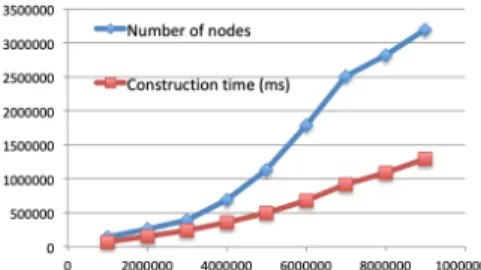
To confirm thescalability of our loading process, we loaded our YAGO subset by slices of 1M triples and recorded after each slice the number of nodes and the running time until that point. Here, we disabled entity extraction, since the graph is already well-structured and well-typed, as well as matching; by definition, each RDF URI or literal is only equivalent to itself. Thus the per-graph value creation policy suffices to copy the RDF graph structure in our graph. Figure 5 shows that the loading time grows quite linearly with the data volume. The figure also shows the cumulated number of different RDF nodes; between 4M and 7M, the number of nodes increases more rapidly, which, in turn, causes a higher cost (higher slope of the loading time) due to more disk writes.

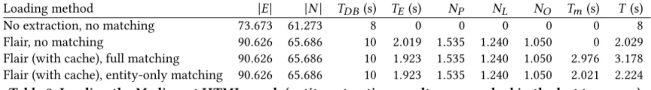
Next, we quantify the impact ofextraction (Section 4) and of matching (Section 6). For this, we rely on the HTML corpus, which is rich in mentions of people, locations and organizations. For ref-erence, we first load this graph without extraction, nor matching. Then, we load it with Flair extraction, and, respectively: without matching; with matching as described in Section 6; and with match-ing from which we exclude the node pairs where no node is an entity (that is, the “short string” and the “long string” comparisons). Table 3 shows the results. Besides the metrics already introducesd, we report: 𝑇_𝐸, the time to extract entities; the numbers 𝑁_𝑃, 𝑁_𝐿, and 𝑁_𝑂of extracted people, locations and organization entities; and the matching time 𝑇_𝑚. The latter includes the time to update the database to modify node representatives (this also requires two queries) and to create similarity edges. Table 3 shows the first Flair entity extraction dwarves the data storage time. Second, the corpus features a significant number of entities (more than 4.000). Third, matching is also quite expensive, due to the computation of the similarity functions on pairs of node labels and the many read/write operations required in our architecture. Finally, a constant aspect in all the experiments we performed is thatthe largest share of similarity comparison costs is incurred by comparisons among (long and short) strings, not entities; this is because strings are more nu-merous. Non-entity strings rarely match, and the most significant connections among datasets are on entities. Therefore, we believe good-quality graphs can be obtained even without string compar-isons. In Table 3, avoiding it allows us to significantly reduce the total time by about 33%.

8.3

Table extraction from PDF documents

Our approach for identifying and extracting bidimensional tables from PDF documents (Section 3.1) customizes and improves upon the Camelot library to better detect data cells and their headers. We

present here an evaluation of the quality of our extraction, using metrics adapted from the literature [23]. Specifically, based on a corpus of PDFs labeled with ground truth values [24], we measure the precision and recall of three tasks: (𝑖 )table recognition (REC) is measured on the list of tokens recognized as belonging to the table; (𝑖𝑖 )table structure detection (STR) is measured on the adjacency relations of cells, i.e. each cell is represented by its content, and its nearest right and downwards neighbors; (𝑖𝑖𝑖 )table interpretation (INT) quantifies how well are represented the headers of a cell; a cell is correctlyinterpreted if its associated header cells are correctly identified. Precision and recall are measured to reflect the full or partial matching of headers.

We aggregate the measures over the 55 documents contained in the above-mentioned dataset and we show the results in Table 4. The table shows that the quality of table recognition and table structure is quite good, though not allowing yet for full automation. The relatively low performance on the last task can be explained by the variety of styles in header construction, which could be better tackled by a supervised learning algorithm.

8.4

Named-Entity Recognition

Due to the unavailability of an off-the-shelf, good-quality entity ex-tractor for French text, we decided to train a new model. To decide the best NLP framework to use, we experimented with the Flair [1] and SpaCy (https://spacy.io/) frameworks. Flair allowscombining several embeddings, which can lead to significant quality gains. Fol-lowing [1], after testing different word embedding configurations and datasets, we trained a Flair model usingstacked forward and backward French Flair embeddings with French fastText embeddings on the WikiNER dataset. We will refer to this model asFlair-SFTF. Below, we describe aqualitative comparison of Flair-SFTF with the French Flair and SpaCytrained models. The French pre-trained Flair model is pre-trained with the WikiNER dataset, and uses French character embeddings trained on Wikipedia, and French fastText embeddings. As for SpaCy, two pre-trained models are available for French: a medium (SpaCy-md) and a small one (SpaCy-sm). They are both trained with the WikiNER dataset and the same parameterization. The difference is thatSpaCy-sm does not include word vectors, thus, in general,SpaCy-md is expected to perform bet-ter, since word vectors will most likely impact positively the model performance. Our evaluation also includes the model previously present in ConnectionLens [14], trained usingStanford NER [18], with the Quaero Old Press Extended Named Entity corpus [20].

We measured the precision, recall, and 𝐹 1-score of each model us-ing theconlleval evaluation script, previously used for such tasks10. conlleval evaluates exact matches, i.e., both the text segment of the proposed entity and its type, need to match “gold standard” an-notation, to be considered correct. Precision, recall, and 𝐹 1-score (harmonic mean of precision and recall) are computed for each named-entity type. To get an aggregated, single quality measure, conlleval computes the micro-average precision, recall, and 𝐹 1-score over all recognized entity instances, of all named-entity types.

For evaluation, we used the entire FTBNER dataset [46]. We pre-processed it to convert its entities from the seven types they used, to the three we consider, namely, persons, locations and organizations.

10

The script https://www.clips.uantwerpen.be/conll2002/ner/ has been developed and shared in conjunction with the CoNLL (Conference on Natural Language Learning).

Loading method |𝐸 | |𝑁 | 𝑇_{𝐷 𝐵}(s) 𝑇_𝐸(s) 𝑁_𝑃 𝑁_𝐿 𝑁_𝑂 𝑇𝑚(s) 𝑇 (s)

No extraction, no matching 73.673 61.273 8 0 0 0 0 0 8 Flair, no matching 90.626 65.686 10 2.019 1.535 1.240 1.050 0 2.029 Flair (with cache), full matching 90.626 65.686 10 1.923 1.535 1.240 1.050 2.976 3.178 Flair (with cache), entity-only matching 90.626 65.686 10 1.923 1.535 1.240 1.050 2.021 2.224 Table 3: Loading the Mediapart HTML graph (entity extraction results were cached in the last two rows).

pdfXtr Precision Recall 𝐹 1 LOC 70.16% 76.06% 72.02% STR 71.48% 73.52% 71.68% INT 40.51% 40.01% 39.64% Overall 60.72% 63.20% 61.12% Table 4: Quality of pdfXtr extraction algorithm. After pre-processing, the dataset contains 12K sentences and 11K named-entities (2K persons, 3K locations and 5K organizations).

Flair-SFTF Precision Recall 𝐹 1 LOC 59.52% 79.36% 68.02% ORG 76.56% 74.55% 75.54% PER 72.29% 84.94% 78.10% Micro 69.20% 77.94% 73.31% Flair-pre-trained Precision Recall 𝐹 1 LOC 53.26% 77.71% 63.20% ORG 74.57% 75.61% 75.09% PER 71.76% 84.89% 77.78% Micro 65.55% 77.92% 71.20% SpaCy-md Precision Recall 𝐹 1 LOC 55.77% 78.00% 65.04% ORG 72.72% 54.85% 62.53% PER 53.09% 74.98% 62.16% Micro 61.06% 65.93% 63.40% SpaCy-sm Precision Recall 𝐹 1 LOC 54.92% 79.41% 64.93% ORG 71.92% 53.23% 61.18% PER 57.32% 79.19% 66.50% Micro 61.25% 66.32% 63.68% Stanford NER Precision Recall 𝐹 1 LOC 62.17% 69.05% 65.43% ORG 15.82% 5.39% 8.04% PER 55.31% 88.26% 68.00% Micro 50.12% 40.69% 44.91% Table 5: Quality of NER from French text.

The evaluation results are shown in Table 5. All models perform better overall than theStanford NER model previously used in ConnectionLens [14, 15], which has a micro 𝐹 1-score of about 45%. TheSpaCy-sm model has a slightly better overall performance thanSpaCy-md, with a small micro 𝐹 1-score difference of 0.28%. SpaCy-md shows higher 𝐹 1-scores for locations and organizations, but is worse on people, driving down its overall quality. All Flair models surpass the micro scores of SpaCy models. In particular, for people and organizations, Flair models show more than 11% higher 𝐹 1-scores than SpaCy models. Flair models score better

on all named-entity types, except for locations when comparing the SpaCy models, specifically, with thepre-trained. Flair-SFTF has an overall 𝐹 1-score of 73.31% and has better scores than theFlair-pre-trained for all metrics and named-entity types, with the exception of the recall of organizations, lower by 1.06%. In conclusion,Flair-SFTF is the best NER model we evaluated.

Finally, we studyextraction speed. The average time to extract named-entities from a sentence is: for Flair-SFTF 22𝑚𝑠 , Flair-pre-trained 23𝑚𝑠 , SpaCy-md 9𝑚𝑠 , SpaCy-sm 9𝑚𝑠 , and Stanford NER 1𝑚𝑠 . The quality of Flair models come at a cost: they take, on average, more time to extract named-entities from sentences. SpaCy extraction is about twice as fast, and Stanford NER much faster. Note thatextraction time is high, compared with other processing costs; as a point of comparison, on the same hardware, tuple access on disk through JDBC takes 0.2 to 1 ms (and in-memory processing is of course much faster). This is whyextraction cost is often a significant component of the total graph construction time.

8.5

Disambiguation

We now move to the evaluation of the disambiguation module. As mentioned in Section 5, our module works for both English and French. The performance for English has been measured on the CoNLL-YAGO dataset [27], by the developers of Ambiverse. They report a micro-accuracy of 84.61% and a macro-accuracy of 82.67%. To the best of our knowledge, there is no labeled corpus for entity disambiguation in French, thus we evaluate the performance of the module on the FTBNER dataset previously introduced. FTBNER consists of sentences annotated with named entities. The disam-biguation module takes a sentence, the type, and offsets of the entities extracted from it, and returns for each entity either the URI of the matched entity or an empty result if the entity was not found in the KB. In our experiment, 19% of entities have not been disambiguated, more precisely 22% of organizations, 29% of persons, and 2% of locations. For a fine-grained error analysis, we sampled 150 sentences and we manually verified the disambiguation results (Table 6). The module performs very well, with excellent results for locations (𝐹 1= 98.01%), followed by good results for organizations (𝐹 1= 82.90%) and for persons (𝐹 1 = 76.62%). In addition to these results, we obtain a micro-accuracy of 90.62% and a macro-accuracy of 90.92%. The performance is comparable with the one reported by the Ambiverse authors for English. We should note though that the improvement for French might be due to our smaller test set.

Precision Recall 𝐹 1 LOC 99.00% 97.05% 98.01% ORG 92.38% 75.19% 82.90% PER 75.36% 77.94% 76.62% Micro 90.51% 82.94% 86.55%

The average time of disambiguation per entity is 347 ms, which isvery significant (again when compared with database access through JDBC of .2 to 2 ms). This is mostly due to the fact that the disambiguator is deployed as a Web service, incurring a client-server communication overhead for making a WSDL call. At the same time, as explained in Section 5, the disambiguation task itself involves large and costly resources; its cost is high, and directly correlated with the number of entities in the datasets. In our current platform, users can turn it on or off.

Experiment conclusion Our experimens have shown that het-erogeneous datasets can be integrated with robust performance in persistent graphs, to be explored and queried by users. We will continue work to optimize the platform.

9

RELATED WORK AND PERSPECTIVES

Our work belongs to the area ofdata integration [16], whose goal is to facilitate working with different databases (or datasets) as if there was only one. Data integration can be achieved either in a warehouse fashion (consolidating all the data sources into a single repository), or in amediator fashion (preserving the data in their original repository, and sending queries to a mediator module which distributes the work to each data source, and finally combines the results). Our initial proposal to the journalists we collaborated with was a mediator [9], where users could write queries in an ad-hoc language, specifying which operations to be done at each source (using, respectively, SQL for a relational source, SOLR’s search syntax for JSON, and SPARQL for an RDF source). This kind of integration through a source-aware language has been successfully explored in polystore systems [4, 32]. In the past, we had also experimented with a mixed XML-RDF language for fact-checking applications [21, 22]. However, the journalists’ feedback has been that the installation and maintenance of a mediator over several data sources, and querying through a mixed language, were very far from their technical skills. This is why here, we (𝑖 ) pursue a warehouse approach; (𝑖𝑖) base our architecture on Postgres, a highly popular and robust system; (𝑖𝑖𝑖 ) simplify the query paradigm to keyword querying.

Because of the applicative needs, ConnectionLens integrates a wide variety of data sources: JSON, relational, RDF and text since [14], to which, since our report [15], we added XML, mul-tidimensional tables, and the ability to extract information from PDF documents. We integrate such heterogeneous content in a graph; from this viewpoint, our work recalls the production of Linked Data. A significant difference is that we do not impose that our graph is RDF, and we do not assume, require, or use a domain ontology. The latter is because adding data to our tool should be as easy as dropping a JSON, XML or text file in an application; the overhead of designing a suitable ontology is much higher and requires domain knowledge. Further, journalists with some tech-nical background found “generic” graphs, such as those stored in Neo4J, more straightforward and more intuitive than RDF ones; this discourages both converting non-RDF data sources into RDF and relying on an ontology. Of course, our graphs could be exported in RDF; and, in different application contexts, Ontology-Based Data Access [10, 11, 34] brings many benefits. Another difference is the pervasive application of Information Extraction on all the values in our graph; we discuss Information Extraction below.

Graphs are also produced whenconstructing knowledge bases, e.g., Yago [38, 51]. Our settings is more limited in that we are only allowed to integrate a given set of datasets that journalists trust. Harvesting information from the World Wide Web or other sources whose authorship is not well-controlled was found risky by journalists who feared a “pollution” of the database. Our choice has therefore been touse a KB only for disambiguation and accept (as stated in Section 1) that the KB does not cover some entities found in our input datasets. Our simple techniques for matching (thus, connecting) nodes are reminiscent of data cleaning, entity resolution [44, 49], and key finding in knowledge bases, e.g. [50]. Much more elaborate techniques exist, notably, when the data is regular, its structure is known and fixed, an ontology is available, etc.; none of these holds in our setting.

Pay-as-you-go data integration refers to techniques whereby data is initially stored with little integration effort and can be better in-tegrated through subsequent use. This also recalls "database crack-ing" [3, 29], where the storage is re-organized to better adapt to its use. We plan to study adaptive stores as part of our future work.

Dataspaces were introduced in [19] to designate “a large number of diverse, interrelated data sources”; The authors note the need to support data sources of heterogeneous data models, and blend query and search, in particular through support for keyword search. Google’s Goods system [26] can be seen as a dataspace. It extracts metadata about millions of datasets used in Google, including sta-tistics but also information about who uses the data when. Unlike Goods, our focus is on integrating heterogeneous data in a graph. Goods is part of thedata lake family, together with products from e.g., IBM and Microsoft. Our approach can be seen as consolidating a highly heterogeneous data lake in a single graph; we consider scaling up through distribution in the near future.

Information extraction (IE) provides techniques to automatically extract structured information such as entities, relationships be-tween entities, unique identifiers of entities, and attributes describ-ing entities from unstructured sources [47]. The followdescrib-ing two IE tasks are particularly relevant in our context.

Named-Entity Recognition (NER, in short) is the task of identify-ing phrases that refer to real-world entities. There exist a variety of NER tools. Firstly, we have web services such as Open Calais11, Watson NLU12 etc.; such services limit the requests in a given time interval, making them less suitable for our needs. Libraries include Stanford NER [18] from Stanford CoreNLP [40], Apache OpenNLP13, SpaCy, KnowNER [48] from the Ambiverse framework, and Flair [1]. These open-source libraries can be customized; they all support English, while Spacy and Flair also support French. These NER tools use supervised techniques such as conditional random fields (Stanford NER) or neural architectures (Flair); text is repre-sented either via hand-crafted features or using word embeddings. We adopted Flair since it is shown to perform well14.

Entity disambiguation aims at assigning a unique identifier to entities in the text. In comparison to NER, there exist far fewer tools for performing disambiguation. From the tools mentioned above, the web-services that perform disambiguation are Gate Cloud and

11

https://permid.org/onecalaisViewer

12

https://www.ibm.com/cloud/watson- natural- language- understanding

13

https://opennlp.apache.org/

14