In-situ measurement of reactive hydrocarbons at Hohenpeissenberg with comprehensive gas chromatography (GCxGC-FID): use in estimating HO and NO<sub>3</sub>

(1)

HAL Id: hal-00302083

https://hal.archives-ouvertes.fr/hal-00302083

Submitted on 29 Aug 2006

HAL is a multi-disciplinary open access

archive for the deposit and dissemination of sci-entific research documents, whether they are pub-lished or not. The documents may come from teaching and research institutions in France or abroad, or from public or private research centers.

L’archive ouverte pluridisciplinaire HAL, est destinée au dépôt et à la diffusion de documents scientifiques de niveau recherche, publiés ou non, émanant des établissements d’enseignement et de recherche français ou étrangers, des laboratoires publics ou privés.

In-situ measurement of reactive hydrocarbons at

Hohenpeissenberg with comprehensive gas

chromatography (GCxGC-FID): use in estimating HO

and NO3

S. Bartenbach, J. Williams, C. Plass-Dülmer, H. Berresheim, J. Lelieveld

To cite this version:

S. Bartenbach, J. Williams, C. Plass-Dülmer, H. Berresheim, J. Lelieveld. In-situ measurement of re-active hydrocarbons at Hohenpeissenberg with comprehensive gas chromatography (GCxGC-FID): use in estimating HO and NO3. Atmospheric Chemistry and Physics Discussions, European Geosciences Union, 2006, 6 (4), pp.8155-8188. �hal-00302083�

(2)

ACPD

6, 8155–8188, 2006 Measurement of VOCs with GCxGC-FID: estimating HO+ NO₃ S. Bartenbach et al. Title Page Abstract Introduction Conclusions References Tables Figures J I J I Back Close

Full Screen / Esc

Printer-friendly Version

Interactive Discussion Atmos. Chem. Phys. Discuss., 6, 8155–8188, 2006

www.atmos-chem-phys-discuss.net/6/8155/2006/ © Author(s) 2006. This work is licensed

under a Creative Commons License.

Atmospheric Chemistry and Physics Discussions

In-situ measurement of reactive

hydrocarbons at Hohenpeissenberg with

comprehensive gas chromatography

(GCxGC-FID): use in estimating HO and

NO

₃

S. Bartenbach1, J. Williams1, C. Plass-D ¨ulmer2, H. Berresheim2, and J. Lelieveld1

1

Max-Planck-Institute for Chemistry, J.J. Becher Weg 27, 55128 Mainz, Germany

2

Deutscher Wetterdienst, Meteorologisches Observatorium Hohenpeissenberg, Albin-Schwaiger-Weg 10, 82382 Hohenpeissenberg, Germany

Received: 22 May 2006 – Accepted: 11 June 2006 – Published: 29 August 2006 Correspondence to: J. Williams (williams@mpch-mainz.mpg.de)

(3)

ACPD

Full Screen / Esc

Interactive Discussion

Abstract

During a field campaign at the Meteorological Observatory Hohenpeissenberg (MOHp) in July 2004, VOCs were measured using GCxGC-FID. Comparison to routinely made GC-MS measurements showed good agreement for a variety of anthropogenic and biogenic ambient VOCs ranging in concentration from below the detection limit

5

(0.1 pmol mol−1) to 180 pmol mol−1. Pronounced diurnal cycles were found for both the biogenic and anthropogenic compounds, driven for the most part by the daily rise and fall of the boundary layer over the station. For the reactive compounds (lifetimes

<2 days), a significant, non-zero dependency of the variability on lifetime was found,

indicating that chemistry (as opposed to transport alone) was playing a role in

deter-10

mining the ambient VOC concentrations. The relationship was exploited using a single-variate analysis to derive a daytime mean value of HO (5.3±1.4×106molecules cm−3, which compares well to that measured at the site, 3.2±2.3×106molecules cm−3. The analysis was extended to the night time data to estimate concentrations for NO₃ (1.47±0.2×108molecules cm−3), which is not measured at the site. The feasibility of

15

this approach for environments dominated by emissions of short-lived VOCs to esti-mate ambient levels of radical species is discussed.

1 Introduction

Volatile organic compounds (VOCs) play an important role in tropospheric air chem-istry and are emitted to the atmosphere from a variety of anthropogenic and biogenic

20

sources (Williams, 2004, and references therein). Some of these compounds can have a direct impact on human health and the environment (Fenger, 1999), while further VOC species can have an indirect impact by undergoing a series of atmospheric ox-idation reactions in the presence of NO_x (NO and NO₂) to produce O₃ which is toxic to both humans and plants (Jacobson, 2002). Removal of VOCs from the atmosphere

25

(4)

ACPD

Full Screen / Esc

Interactive Discussion may also be significant for certain species under certain conditions. Through oxidation,

the VOCs are converted into more polar and hydrophilic forms, which makes these photooxidation products more susceptible to wet removal by rain or dry deposition on surfaces. The combined efficiency of the physical and chemical removal processes define the atmospheric residence time τ, i.e. the time needed for a compound’s initial

5

concentration in the atmosphere to be reduced to 1/e times the initial concentration (Finlayson-Pitts and Pitts, 2000).

To investigate the emission, distribution, and oxidation of VOCs in the atmosphere it is essential that accurate measurements or their concentrations are made. In this study we have applied a GCxGC-FID comprehensive gas chromatography system, to

10

determine ambient mixing ratios of VOCs at the Hohenpeissenberg Global Atmosphere Watch (GAW) Observatory, Germany (http://www.dwd.de/gaw). The relatively new technique of GCxGC (also termed two-biogenic VOCs are compared.dimensional gas chromatography) has been shown previously to provide superior separation power and improved detection limits compared to standard GC methods (one-dimensional gas

15

chromatography or GC-FID) in the analysis of complex oil or flavour samples (Beens et al., 2000; Blomberg et al., 1997; Marriott et al., 2000). More recently, GCxGC has also been successfully applied to the analysis of C₅–C₁₅ VOCs in air samples (Lewis et al., 2000; Xu et al., 2003a and b). In this study a GCxGC-FID system was operated in parallel with a conventional GC-MS system at Hohenpeissenberg during July 2004,

20

and the results for selected anthropogenic and biogenic VOCs compared. The tempo-ral trends and diurnal cycles of these VOCs will be presented and discussed in terms of sources and local meteorology.

The atmospheric variability of the VOCs measured by the GCxGC system was also examined as a function of their chemical residence time. Many previous studies have

25

demonstrated the utility of this approach in assessing data quality as well as garnering valuable information on VOC sources and sinks (Junge, 1974; Jobson et al., 1998, 1999; Williams et al., 2000). Intuitively, we may expect a high variability from species that are most rapidly removed from the atmosphere. In contrast, long-lived species

(5)

ACPD

Full Screen / Esc

Interactive Discussion are relatively insensitive to transport time differences between their source and point of

measurement, and hence exhibit smaller ranges in measured concentration (i.e. vari-ability). Thus an approximate inverse relationship would be expected between variabil-ity and residence time for VOC species, provided the source and sink distributions are similar. It has been found empirically that for studies of VOCs with lifetimes between

5

a few days to a few months, the expression (1) below gives tractable results (Jobson et al., 1998). Here variability is expressed as the standard deviation σ of the natural logarithm of all concentrations X in a dataset i.e. σ ln(X); τ is the chemical lifetime; and

A and b empirical fitting parameters.

σ ln(X)= Aτ−b (1)

10

It has been further shown that the exponent b indicates the proximity of the measure-ment to the source region; b=0 indicates a nearby source and no dependence of vari-ability on chemistry; whereas b=0.5 indicates a remote source, where the variability is significantly influenced by the chemistry. Several groups have used this relationship to derive estimates of the ambient HO radical concentration (Williams et al., 2000, 2001;

15

Karl et al., 2001). Since the HO radical is highly reactive and ambient concentrations are small, (typically of the order of 1×106molecules cm−3or 0.04 pmol mol−1), HO con-centrations are difficult to measure. Hohenpeissenberg where the present study was performed is the only station in the world presently measuring HO on a routine basis (e.g. Berresheim et al., 2000; Rohrer and Berresheim, 2006). Although HO

concen-20

trations and seasonal dependencies derived through the variability analysis have been shown to be reasonably accurate (Williams et al., 2000, 2001; Karl et al., 2001), such estimates have never previously been compared with an in-situ measurement. The interpretation of a variability derived HO value is also not easy to comprehend. Previ-ously such HO values have been interpreted as the average HO acting on the air parcel

25

along the back trajectory. However, just how far back along the back trajectory should be considered is not clear since the HO values are derived from VOCs with a wider range of lifetimes and hence regions of influence. To clarify the interpretation and to

(6)

ACPD

Full Screen / Esc

Interactive Discussion examine the method we have applied the variability analysis to short-lived compounds

(0–2 days), for which the effects of the sources and sinks are local. We then compare the variability derived HO value with the HO measured in-situ. An extension of the method to determine the nocturnal oxidant NO₃is also explored.

2 Experimental

5

2.1 Site description and meteorology

The field campaign (HOHenpeissenberg Photochemistry EXperiment) was conducted in July 2004 at the Meteorological Observatory Hohenpeissenberg (MOHp), southern Germany (47◦480N, 11◦010E). This station is operated by the German Weather Service (Deutscher Wetterdienst, DWD). As part of its Global Atmosphere Watch program

long-10

term measurements of VOCs (Plass-D ¨ulmer et al., 2002) and HO (Berresheim et al., 2000) are conducted and complemented by campaign studies focussing on particle and oxidant formation processes (e.g. Acker et al., 2006; Handisides et al., 2003; Birmili et al., 2002, 2000). The site is located on a hilltop (elevation of 980 m a.s.l.) in a rural agricultural and forested area, approximately 40 km north of the Alps. It surmounts the

15

adjacent countryside by approximately 300–400 m with the slopes mostly covered by coniferous forest and grassland dominating in the valley below. In the north-to-south foothills the village of Hohenpeissenberg is located with typical country road traffic. The nearest major city is Munich, at a distance of about 70 km to the northeast. Main wind direction was south to southwest.

20

During HOHPEX, VOC concentrations at the Hohenpeissenberg station were strongly influenced by the diurnal variation in height of the atmospheric boundary layer (BL) and atmospheric turbulence (e.g. Handisides et al., 2003). During the night the boundary layer often formed below the measurement station, isolating the station from nocturnal emissions in the boundary layer and leaving it in the residual layer under

25

the influence of air masses from the previous day (before 10 July and after 17 July). 8159

(7)

ACPD

Full Screen / Esc

Interactive Discussion However, on average higher wind speeds during the middle part of the campaign may

have prevented the nocturnal inversion layer to develop, thus night time VOC mixing ratios were higher and fluctuating (between 11 July and 16 July). After sunrise the BL was rising and reached the station at mid-morning hours with significant advection of VOCs from both anthropogenic and biogenic emissions. Between about noon and

5

16:00 CEST, Hohenpeissenberg was situated in the well-mixed BL, and during this time transport processes played an important role for VOCs measured at the station.

Weather conditions during the campaign ranged from warm and sunny in the begin-ning to cold and rainy for the main part before reverting to warmer conditions at the end. A selection of meteorological parameters is shown in Fig. 1. The highest

tem-10

perature measured was around 25◦C; the lowest, 7◦C, was reached at night during the middle section of the campaign. The cooler days between the 11 and 14 July showed temperatures mostly below 15◦C, and the weather was generally foggy, with short rain showers and an overcast sky.

2.2 Gas chromatographic systems

15

The in-situ GCxGC-FID measurement system used during the campaign includes a gas chromatograph (GC6890, Agilent, Wilmington, USA) equipped with a flame ioni-sation detector (FID) and a jet-modulator (Zoex, Lincoln, USA); a flow controller and a thermal desorber (Markes Int., Pontyclun, UK). The system has been described in detail elsewhere (Xu et al., 2003b).

20

In GCxGC, two columns with different selectivity, in this case produced by a non-polar and a non-polar stationary phase, respectively, are connected in series. The entire sample is undergoing separation in both dimensions unlike heartcut-GC, where only parts of the sample are subjected to further separation. The sample is separated on the first column based on volatility, small fractions of the effluent are retained in the

25

modulation part at the end of this column for a short period of time. Following the release, the compounds are injected into the second column where they are quickly separated based on their polarity and subsequently detected.

(8)

ACPD

Full Screen / Esc

Interactive Discussion An approximately 15 m long, 12.7 mm diameter Teflon inlet line was attached to a

rail-ing on the top of the measurement platform (1000 m a.s.l.). The line itself was shielded from sunlight inside an opaque tube, leading from the platform along the outside wall to the laboratory. The volume flow through the main inlet was set to 3.2 L min−1, result-ing in a residence time of circa 20 sec. Ambient air was drawn from the fast flow into

5

the cold trap through a 3.2 mm Teflon line at a rate of 50 ml min−1 using a membrane pump (KNF Laboport, Germany). The pertinent sampling and analysis parameters are summarised in Table 1. Blanks were conducted by focussing helium 6.0 (Messer-Griesheim, Germany) on the cold trap with the same parameters as shown for ambient air. The adsorbent trap temperature was set to 25◦C, as the weather was generally

10

humid throughout the campaign and condensation of water vapour inside the trap had to be strictly avoided. After the sample was accumulated, the trap was purged with helium for 10 min to remove traces of water vapour, then heated up to 200◦C to inject the focussed compounds onto the column. For complete desorption, this temperature was maintained for 5 min. The column set used during the field campaign was a

non-15

polar DB-5 (Agilent, Waldbronn, Germany) in the first dimension and a polar BPX-50 (SGE Deutschland, Darmstadt, Germany) in the second dimension. Calibration was achieved based on a 74 compound VOC standard (Apel-Riemer, CT, USA). A simi-lar standard from the same company is routinely used in the Hohenpeissenberg GAW VOC programme. Laboratory multipoint calibrations were accomplished earlier and

re-20

vealed for all VOCs a good linear dependency of peak area to the respective compound mass. Based on this stability, a one-point calibration of 200 ml standard was carried out every second day throughout the rainy period, whereas the sunny period of four days towards the end of the campaign was only disrupted for blanks. Blanks were taken every third day and showed no high levels for the compounds discussed.

Commer-25

cially available software for peak detection and integration was found to be slow and unsuitable. An integration procedure was written within IgorPro 4.0 software (Wave-Metrics Inc., USA) to calculate the volume of each peak and allow semi-automatic data analysis processing of selected substances.

(9)

ACPD

Full Screen / Esc

Interactive Discussion Continuous daily GC-MS measurements were conducted at the observatory within

the GAW programme at 1 h time resolution and 20 min sampling integration. The sam-pling for the GC-MS measurements of the MOHp was done from a permanently in-stalled 10 m×40 mm I.D. glass tube flushed with ambient air at a rate of 1 m3min−1. The sample was accumulated from this glass tube by means of a 1 m, 1/800 silcosteel

5

tube for 20 min at 75 ml min−1. The sampling and analysis details are given in Table 2. The measurement uncertainties ranged between 6%–10% for the GCxGC-FID and be-tween 11%–34% for the GC-MS. The limits of detection ranged from 0.1 pmol mol−1 to 2.8 pmol mol−1for the GCxGC-FID and 0.5 and 2.6 pmol mol−1for the GC-MS.

The atmospheric HO was measured using the selected ion/chemical ionisation mass

10

spectrometer (SI/CIMS) described by Berresheim et al. (2000). O₃ was determined with a UV absorption instrument (Thermo Env., USA).

3 Results

3.1 Comparison of GCxGC-FID and GC-MS measurements

During the campaign, from 7 July to 18 July 2004, the GCxGC-FID

(Max-Planck-15

Institute) measurements were intercompared with the concurrent GC-MS measure-ments. A total of 162 and 130 measurements were made with the GC-MS and the GCxGC-FID, respectively. Included in the comparison were the anthropogenic com-pounds hexane, heptane, octane, nonane, ethylbenzene, the co-eluting p-/m-xylene and o-xylene as well as the biogenic compounds α- and β-pinene, 3-carene,

cam-20

phene and eucalyptol. Figure 2 shows a time series of ethylbenzene, octane and

α-pinene for both instruments (red points GCxGC-FID and black points GC-MS). The

markers represent the middle of the sampling time, the upper and lower bars the total measurement uncertainty for the depicted VOC.

Generally there was good agreement between measured VOC concentrations. Slight

25

(10)

ACPD

Full Screen / Esc

Interactive Discussion the GC-MS sampled for 20 min, while air was collected for 60 min in the GCxGC-FID

system. There is generally good agreement for the reactive biogenic VOC measure-ments (see e.g. α-pinene), although no O₃scrubber was applied for GCxGC sampling but a Na₂S₂O₃impregnated filter was used in the GC-MS sampling line. According to a study, the sampling of reactive terpenes on Tenax in presence of O₃leads to losses if

5

no O₃scrubber is used (Calogirou et al., 1996). However, the terpenes discussed here are only slightly or not at all affected, although it should be noted that the most reactive terpenes towards O₃, e.g. terpinolene are not included.

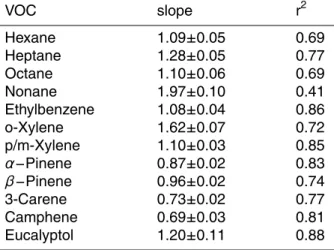
The data from both systems were correlated using orthogonal distance regression (ODR) instead of the standard linear regression (SLR). With this method, all data points

10

are assumed to have an equal weight and the orthogonal distance between the fitted line and the individual data points is minimised, whereas in the SLR only the distance in y-direction is optimised. Good correlations were found for the examined compounds, with the exception of nonane which was caused by low concentrations close to the detection limit, see Table 3.

15

3.2 Diel cycles

Average diel cycles of the GCxGC-FID measured VOCs α-pinene and sabinene (bio-genic); and octane and ethylbenzene (anthropogenic), are shown in Fig. 3. The black line illustrates the hourly mean mixing ratio, the lower and upper bars represent the minimum and maximum measured values respectively, and the dotted line the

me-20

dian value. The effects of the diurnally changing boundary layer height described in Sect. 2.1 can be observed in the mean values for all measured VOCs in the late morn-ing around 09:00 CEST, when the ascendmorn-ing BL reaches the station. In the night, the usually low BL and the stations’ isolation from the ground based sources leads to lower mean VOC levels.

25

Biogenically emitted compounds followed a diurnal profile similar to that of α-pinene. The mixing ratios for all biogenic VOCs measured with GCxGC-FID are shown in Fig. 4. For biogenic species the mean mixing ratios increased slowly after sunrise, and

(11)

ACPD

Full Screen / Esc

Interactive Discussion abruptly as the BL reached the elevation of the site. An additional maximum around

14:00 CEST was also observed for α- and β-pinene later in the afternoon, whereas the other measured terpenes remain at a constant high level or decrease slowly. Dif-ferent from the other monoterpenes shown, sabinene concentratios are close to zero at night. The diurnal cycles are driven by the dependence of the emission on

inso-5

lation and temperature. With mostly mixed spruce forest surrounding the station, the most abundant biogenic compounds were α- and β-pinene. These VOCs, along with camphene and 3-carene, are known to be emitted by spruce trees (Street et al., 1996; Fulton et al., 1998). Continuous elevated mixing ratios for these terpenes have been detected on some of the cooler nights, indicating a constant release from the storage

10

pools in the needles (Fuentes et al., 2000) although α-pinene seems to have a larger diurnal dependence than β-pinene, with significantly higher mixing ratios during day-time. In contrast, sabinene has been reported to be mainly emitted by beech and other deciduous trees (Tollsten et al., 1996). At Hohenpeissenberg, sabinene is almost only observed during daytime, suggesting that the emission was strongly light dependent.

15

This phenomenon has been observed in earlier studies (Staudt et al., 1997; Bertin et al., 1997) and was also reported for beech and birch leaves, where emission in the dark gradually decreased for all measured monoterpenes at a constant temperature (Hakola et al., 2001). Eucalyptol also makes up a significant proportion of the to-tal monoterpenes (Plass-Duelmer and Berresheim1). Previous studies have indicated

20

that it is emitted from various plants such as rape, birch, spruce, hornbeam and grass-land (K ¨onig et al., 1995; Hakola et al., 2003; Kirstine et al., 1998). The emission from grassland is reported to be particularly strong at elevated temperatures and after mow-ing (K ¨onig et al., 1995). Short-term increases in mixmow-ing ratios for all monoterpenes have been detected occasionally during the night, mainly in the cold, windy and rainy

25

phase of the field campaign. This indicates a turbulent atmosphere without the

de-1

Plass-Duelmer, C. and Berresheim, H.: On-line GC measurements of atmospheric monoterpenes at the Global Atmosphere Watch observatory Hohenpeissenberg, in prepara-tion, 2006.

(12)

ACPD

Full Screen / Esc

Interactive Discussion velopment of the nocturnal inversion, thus no decoupling between the boundary layer

and the measurement point occurred and the station was still influenced by emissions at ground level or aged residual layer air through vertical and horizontal transport pro-cesses. Additionally, relative humidity and rainfall can exert positive influence on the emission of monoterpenes from pine trees (Schade et al., 1999), a further study

pro-5

posed a connection between contact stimulation and stronger emission of terpenes in Japanese cypresses (Yatagai et al., 1995). Both hypotheses might also be relevant for nocturnal emissions originating from the mixed spruce forest around the Hohen-peissenberg, as the observed wind speed during these nights was mostly higher than 8 m s−1, the humidity was very high and precipitation occurred frequently.

10

The anthropogenic compounds show a slightly different diurnal cycle to the biogenic VOCs, the sum and the fractional contributions are shown in Fig. 5. Main sources for these species can be found in automobile exhaust, gasoline evaporation or solvents. Just as the biogenic compounds, the mean atmospheric mixing ratios for anthropogenic VOCs also peak between 09:00 and 10:00 CEST (with the arrival of the boundary layer

15

at the site), but remain approximately constant at this level until around noon, when the boundary layer is well-mixed. The fluctuating course of the mixing ratios through-out the rest of the day is probably driven by variations in anthropogenic emissions and/or a changing fetch area. The development of a shallow nocturnal BL between 22:00 and 01:00 CEST was accompanied by an almost steady or decreasing level of

20

anthropogenic VOCs during the night, until the BL ascended over the station again the following morning. Like for the biogenic VOCs, fluctuating anthropogenic nighttime mix-ing ratios were occasionally measured (13 to 16 July, see Fig. 2), when the nocturnal BL did not develop as a result of the turbulent atmosphere.

3.3 Lifetime-variability dependence of VOCs

25

In Sects. 2.1 and 3.2 we have shown that in addition to synoptic scale horizontal air mass advection the Hohenpeissenberg site was influenced by diurnal changes in boundary layer height with local air influence prevailing by day and aged local

(13)

ACPD

Full Screen / Esc

Interactive Discussion air by night. Since the biogenic compounds are emitted from the nearby forest

and the sources for the anthropogenic VOCs are also close, we can expect a weak or negligible influence of chemistry on the variability-lifetime relationship. The at-mospheric lifetimes of the VOCs during daytime are mainly dependent on HO and O₃. Both of these species were measured at Hohenpeissenberg and the mean

val-5

ues (1.7×106molecules cm−3 (0.071 pmol mol−1) HO and 1.0×1012molecules cm−3 (42.0 nmol mol−1) O₃ were taken for the plot shown in Fig. 6. These averages were determined over the period when all three instruments were operating, from 7 July to 16 July (Table 4).

The variability of the measured species was obtained according to Jobson et

10

al. (1998), as described in Sect. 1. A relatively high variability can be observed in all biogenic compounds, particularly sabinene (see Fig. 6). The higher variability for sabinene as compared to the other terpenes is possibly caused by it being predomi-nately emitted from deciduous trees (e.g. beech) which exhibit mostly light-dependent emission (Tollsten et al., 1996), in contrast to the conifers which generally emit as a

15

function of temperature and light (Street et al., 1996; Fulton et al., 1998). However, both tree types are found mixed throughout the Hohenpeissenberg forest, therefore we assume that the source location and distribution of all terpenes is sufficiently similar to permit the variability analysis. Moreover in the subsequent more detailed variability analysis we segregate the data into day (high temperature and light) and night (low

20

temperature and no light) to minimise any effect of different source terms as well as of different radical chemistry on the analysis. It is also interesting to note that eucalyptol and β-pinene exibit approximately the same variability although they have longer life-times than the other terpenes analysed, especially at night. Eucalyptol appears to be more variable than expected, possibly indicating an additional sink. Since eucalyptol

25

contains an oxygen atom and is therefore more polar than the other monoterpenes, one may speculate that wet removal or deposition of this compound has occurred. The anthropogenic species, which in this case have relatively long lifetimes, show less variability in their measured concentration. The lifetimes were calculated using the

(14)

re-ACPD

Full Screen / Esc

Interactive Discussion action rate coefficients from Atkinson (1997), Atkinson et al. (1986, 1990), Corchnoy

and Aktinson (1990) and the average measured O₃ and HO concentration, the data was fitted to the previously described function σln(X)=Aτ−b. The coefficients derived for all compounds are A=0.48±0.06 and b=0.24±0.06. If only the biogenically emitted compounds are considered, A=0.45±0.24, and b=0.27±0.20. For only the biogenic

5

VOCs reacting rapidly with both O₃and HO (lifetime <6 h), b increases to 0.75±0.33. Interestingly, the exponent b=0.24 for all VOCs indicates that there is a significant, non-zero dependency of the variability on lifetime for these species at the measurement site, and therefore that chemistry (as opposed to transport alone) is playing some role in determining the ambient concentrations. At first this result may seem surprising

10

as previous studies have shown that sources of alkane emissions near to a point of measurement tend to generate variability in a dataset that is not connected with chem-istry and hence reduce the coefficient b (b≈0) (Jobson et al., 1998). In the case of Hohenpeissenberg the site is surrounded by mixed forest (the source of the biogenic compounds) on all sides. A low value (b=0.18) was found for a VOC dataset, albeit

15

with somewhat longer lifetimes ranging from 1 to 500 days, taken over Harvard forest (Jobson et al., 1999). We interpret this finding as showing that the species measured in the present study are sufficiently reactive to be oxidised on such short temporal and spatial scales that a significant variability-lifetime relationship can develop.

3.4 Estimation of HO radical concentrations

20

As described previously, VOCs can be removed from the atmosphere by HO, NO₃ and O₃. Several studies have demonstrated that when a significant variability-lifetime relationship exists for a suite of VOCs, it can be used to estimate the HO radical con-centration in the atmosphere (e.g. Jobson et al., 1999; Williams et al., 2000; Karl et al., 2001). The general principle is: if measured VOCs react with more than one oxidant

25

(e.g. HO and O₃) and the atmospheric concentration of either one is known (e.g. O₃), it is possible to estimate the concentrations of the other reactant(s), assuming that all reaction rates are known. From the Hohenpeissenberg data set both HO and O₃

(15)

ACPD

Full Screen / Esc

Interactive Discussion surements are available presenting the unique opportunity to test this approach in a

rural continental environment. Assuming the level of one oxidant (here O₃) is known, its concentration is kept constant while that of the “unknown” oxidant species (here HO) is varied. The distribution of the data points on the variability-lifetime plot thus varies as a function of the assumed HO radical concentration and fits with varying degrees

5

are obtained. The goodness of a fit is expressed by the χ2(chi squared) value, which evaluates the correlation of the least squares fit and indicates the discrepancy between the fitting function and the data. A lower χ2indicates a better fit to the data. The as-sumed concentration of the oxidant that gives the best fit to the data is interpreted as the average concentration of the oxidant that has affected the airmass. The standard

10

deviation of the gradient b (Eq. 1) is then used to express the uncertainty in the HO estimate.

This method was applied here first to all VOCs anthropogenic and biogenic, and in a second step to the short-lived VOCs, since both have shown a significant variability-lifetime dependence, despite being close to the sources. An advantage of using

short-15

lived species is that the HO calculated should be comparable to the in-situ HO mea-surements made during the HOHPEX field campaign. This is because the radical chemistry that gives rise to the variability-lifetime dependency must be occurring lo-cally. To investigate this further, two strategies were tested. First the O₃concentration was kept constant at the diurnal average of 1.0×1012molecules cm−3(42.0 nmol mol−1)

20

and the HO concentration was varied. This simulates the common situation where O₃ is measured but HO is not. Secondly we varied O₃ and HO simultaneously to deter-mine whether the VOC variability-lifetime relationship yields reasonable values for both oxidants without assuming a measured value.

To calculate the diel variability and to minimise the influence of changes in the

bound-25

ary layer height, the dataset was divided according to time in two sections (10:00 and 19:30 CEST day; 22:00 and 05:30 CEST night). For comparison it should also be recalled that when both GCxGC-FID and the HO instrument were operational, the average measured daytime HO was found to be 3.2±2.3×106molecules cm−3

(16)

ACPD

Full Screen / Esc

Interactive Discussion (0.13±0.097 pmol mol−1). When O₃ is held at the average mixing ratio and only HO

is varied, for all the measured biogenic and anthropogenic VOCs no best fit (i.e low-est χ2) can be calculated, see Table 4. However, if only the highly reactive biogenic VOCs with similar sources, i.e. the forest surrounding the station, and atmospheric life-times lower than 6 h are considered, the calculated average daytime HO concentration

5

is 5.3± 1.4×106 HO molecules cm−3 (0.22±0.06 pmol mol−1), which is at the upper limit of the HO actually measured. This shows the analysis to be highly sensitive to which species are used in the fitting procedure. In particular, VOC species emitted by the same spatial and temporal source pattern must be used. However, there remain some uncertainties since the fit results strongly depend on the sabinene data point,

10

which, as outlined above, originates from deciduous trees with potentially a different source-variability (light dependent) as compared to the other terpenes analysed here, which originate from coniferous trees (light and temperature dependent). If sabinene is not considered, no significant slope can be determined for the short lived biogenic VOC and variability does not depend on chemical lifetime. It is therefore prudent to

15

include as many terpene compounds as possible with a wide reactivity spectrum in future studies of this kind. The calculated average HO concentration for the whole diurnal GCxGC biogenic VOC dataset, which, unlike the HO instrument, was also op-erating during rainy periods, yields an average of 4.6±1.2×106 HO molecules cm−3 (0.19±0.05 pmol mol−1), see Fig. 7a.

20

For the simultaneous variation of both O₃ and HO no distinct O₃/HO optimum was obtained, instead a ridge of “best guess” HO values for each O₃ concentration is generated. The HO concentration based on the measured O₃ with ±1σ uncer-tainty (1.0±0.2×1012molecules cm−3, 42.0±8.4 nmol mol−1) was between 4.1±1.6 and 6.5±2.6×106molecules cm−3(0.17 to 0.27 pmol mol−1).

25

From the in-situ measurements at MOHp, an average daytime HO concentration of 3.2±2.3×106molecules cm−3 (0.13±0.1 pmol mol−1) was obtained, whereas for the HO estimated from the combined biogenic and anthropogenic VOCs no concentration could be calculated. This is very likely caused by the differences in sources for the

(17)

ACPD

Full Screen / Esc

Interactive Discussion individual species (which generate variability unrelated to chemistry) as well as the low

reactivity of O₃ with the anthropogenic VOCs as compared to the biogenic (Ehhalt et al., 1998). To obtain an estimate for the local concentration of an oxidant, compounds should be selected which are emitted from similar source types and have generally short atmospheric lifetimes, but a sufficient span of reactivity to define the

variability-5

lifetime plot. We should consider, however, the possibility that the agreement found between measured and estimated HO could be coincidental. This would mean that the variability of the selected terpenes is driven by processes other than HO (i.e. source variability or distribution) and the constellation of variabilities fortunately co-incides with the measured HO when this method is applied. To test this requires further studies,

10

ideally where high time resolution measurements of terpenes and HO are made over large homogeneous tracts of vegetation. Large areas of monocultures such as the vast oil palm plantations of Malaysia would be one possibility as these would emit the same species in the same source profile. Another interesting possibility would be the tropical rainforest, if large areas are covered with airborne measurements.

15

3.5 Estimation of NO₃radical concentrations

By day VOC oxidation proceeds mainly through reaction of HO and O₃. However, by night NO₃and O₃are understood to be the most important oxidising species since the main source of HO, photolysis, becomes negligible. Unlike HO, NO₃ was not mea-sured at Hohenpeissenberg, therefore it is particularly interesting to use the VOC data

20

to extract an estimate of the NO₃ concentration. To investigate the levels of NO₃, the variability analysis was applied as before but on the night time data only (from 22:00 to 05:30 CEST). Alas, for this dataset no optimum was found when either O₃was fixed at the measured value or when both O₃ and NO₃ were varied simultaneously. On the other hand, when an HO value was specified (as measured) and the O₃and NO₃

25

radical values varied, a χ2surface could be generated with a maximum for the di ffer-ent O₃ concentrations, but, as with the O₃/HO calculation, without a distinct O₃/NO₃ maximum. Taking the biogenic data only (since the station was mostly cut off from

(18)

an-ACPD

Full Screen / Esc

Interactive Discussion thropogenic sources by night) and adopting the average measured O₃ and HO value

by night (1.0×1012molecules cm−3 and 0.1×106molecules cm−3, respectively) we find a calculated NO₃ value of 1.47 ± 0.2×108molecules cm−3 (6.2±0.8 pmol mol−1), see Fig. 7b.

A recent study of Handisides et al. (2003) during HOPE2000 considered the

pro-5

duction and loss rates of NO₃and assumed an average nocturnal NO₃concentration of 6 pmol mol−1 at Hohenpeissenberg. This value and the value derived in the work presented here is also in general agreement with measurements conducted in the con-tinental boundary layer near Berlin, Germany, which revealed a nocturnal average of 4.6 pmol mol−1(Geyer et al., 2001).

10

4 Conclusions

During the field campaign HOHPEX at the Meteorological Observatory Hohenpeis-senberg (MOHp) in July 2004, anthropogenic and biogenic VOCs were successfully measured using GCxGC-FID. Comparison to routinely conducted GC-MS measure-ments at MOHp during the same period showed that good agreement was obtained for

15

a variety of ambient VOCs ranging in concentration from zero to 180 pmol mol−1. Pronounced diel cycles were found for both the biogenic and anthropogenic com-pounds, driven for the most part by the daily rise and fall of the boundary layer over the station. The mixing ratios of the biogenic species (e.g α- and β-pinene, sabinene, 3-carene, camphene and eucalyptol) were strongly influenced by emissions from the

20

forest in the vicinity of the station. In agreement with previous studies, cool and cloudy days showed generally less terpene emission than warm and sunny days. Diel cycles for the anthropogenic (aromatic and aliphatic) compounds were also found, but with different characteristics to those of the biogenic species. The highest mixing ratios for all VOCs were measured in the morning when the boundary layer rose over the station.

25

The variability-lifetime relationship of the short-lived VOCs has been examined for the first time. The weak but significant b dependence of the measured compounds

(19)

ACPD

Full Screen / Esc

Interactive Discussion showed that although the VOC sources are relatively close, chemistry was playing a

significant role in determining their concentration. The relationship was exploited to es-timate the atmospheric mean HO concentration from the GCxGC-FID VOC measure-ments for comparison with measured HO. The mean daytime HO concentration thus derived is 5.3±1.4×106molecules cm−3 (0.22±0.06 pmol mol−1), slightly higher

com-5

pared to the mean HO measured at MOHp. No distinct optimum for HO and O₃ are found when both O₃and HO are co-varied to estimate oxidant levels. By extending the analysis to the night time data, the mean NO₃radical concentration is estimated to be 1.47±0.2×108 molecules cm−3 (6.2±0.8 pmol mol−1). This appears to represent the limit of what can be extracted from this dataset with its limited temporal resolution and

10

suite of compounds. However, this study indicates the potential to determine the am-bient radical concentrations of HO and NO₃by analysing measured VOC mixing ratios at rural sites surrounded by homogeneous vegetation and unaffected by major pollu-tion. This possibility should be further explored in future studies including fast reacting biogenic species and in-situ HO measurements over a large scale homogeneous

ex-15

cosystem. Particularly suitable in this regard would be monoterpene measurements over a tropical rainforest.

Acknowledgements. The authors are grateful for help by the ORSUM group and the GAW team

at Hohenpeissenberg and to DWD/BMVBS for support of this study. We also thank R. L ¨oscher and the company LECO for their assistance in characterisation of the instrument prior to this

20

work.

References

Acker, K., M ¨oller, D., Wieprech,t W., Meixner, F. X., Bohn, B., Gilge, S., Plass-D ¨ulmer, C., and Berresheim, H.: Strong daytime production of OH from HNO₂at a rural mountain site, Geophys. Res. Lett., L02809, doi:10.1029/2005GL024643, 2006.

25

Atkinson, R.: Gas-phase tropospheric chemistry of organic compounds, J. Phys. Chem. Ref. Data, 26, 215–290, 1997.

(20)

ACPD

Full Screen / Esc

Atkinson, R., Aschmann, S. M., and Arey, J.: Rate constants for the gas-phase reactions of OH and NO₃radicals and O₃ with sabinene and camphene at 296+/−2 K, Atmos. Environ., 24, 2647–2656,1990.

Atkinson, R., Aschmann, S. M., and Pitts, J. N.: Rate constants for the gas-phase reactions of the OH radical with a series of monoterpenes at 294 K, Int. J. Chem. Kinet., 18, 287–299,

5

1986.

Beens, J., Blomberg, J., and Schoenmakers, P. J.: Proper tuning of comprehensive two-dimensional gas chromatography (GCxGC) to optimize the separation of complex oil frac-tions, J. High Resol. Chromatogr., 23, 182–188, 2000.

Berresheim, H., Elste, T., Plass-D ¨ulmer, C., Eisele, F. L., and Tanner, T. J.: Chemical ionization

10

mass spectrometer for long-term measurements of atmospheric OH and H₂SO₄, Int. J. Mass. Spect., 202, 91–109, 2000.

Bertin, N., Staudt, M., Hansen, U., Seufert, G., Ciccioli, P., Foste,r P., Fugit, J.-L., and Torres, L.: Diurnal and seasonal course of monoterpene emissions from Quercus ilex (L.) under natural conditions – Application of light and temperature algorithms, Atmos. Environ., 31, 135–144,

15

1997.

Birmili, W., Berresheim, H., Plass-D ¨ulmer, C., Elste, T., Gilge, S., Wiedensohler, A., and Uhrner, U.: The Hohenpeissenberg aerosol formation experiment (HAFEX): a long-term study in-cluding size-resolved aerosol, H₂SO₄, OH, and monoterpene measurements, Atmos. Chem. Phys., 3, 361–376, 2002.

20

Birmili, W., Wiedensohler, A., Plass-D ¨ulmer, C., and Berresheim, H.: Evolution of newly formed aerosol particles in the continental boundary layer, J. Geophys. Res., 27, 2205–2208, 2000. Blomberg, J., Schoenmakers, P. J., Beens, J., and Tijssen, R.: Comprehensive two-dimensional gas chromatography (GCxGC) and its applicability to the characterization of complex (petro-chemical) mixtures, J. High Resol. Chromatogr., 20, 539–544, 1997.

25

Calogirou, A., Larsen, B. R., Brussol, C., Duana, M., and Kotzias, D.: Decomposition of ter-penes by ozone during sampling on Tenax, Anal. Chem., 68, 1499–1506, 1996.

Corchnoy, S. B. and Atkinson, R.: Kinetics of the gas-phase reactions of OH and NO₃radicals with 2-carene, 1,8-cineole, p-cymene, and terpinolene, Environ. Sci. Technol., 24, 1497– 1502, 1990.

30

Ehhalt, D. H., Rohrer, F., and Wahner, A.: On the use of hydrocarbons for the determination of tropospheric OH concentrations, J. Geophys. Res., 103, 18 981–18 997, 1998.

Fenger, J.: Urban air quality, Atmos. Environ., 33, 4877–4900, 1999.

(21)

ACPD

Full Screen / Esc

Finlayson-Pitts, B. J. and Pitts, Jr. J. N.: Chemistry of the upper and lower atmosphere, Aca-demic Press, 2000.

Fuentes, J. D., Lerdau, M., Atkinson, R., Baldocchi, D., Bottenheim, J. W., Ciccioli, P., Lamb, B., Geron, C., Gu, L., Guenther, A., Shaerkey, T. D., and Stockwell, W.: Biogenic hydrocarbons in the atmospheric boundary layer: A review, Bull. Am. Meteorol. Soc., 81, 1537–1575, 2000.

5

Fulton, D., Gillespie T., Fuentes, J., and Wang, D.: Volatile organic compound emissions from young black spruce trees, Agric. Forest Met., 90, 247–255, 1998.

Geyer, A., Ackermann, R., Dubois, R., Lohrmann, B., M ¨uller, T., and Platt, U.: Long-term observation of nitrate radicals in the continental boundary layer near Berlin, Atmos. Environ., 38, 4733–4747, 2001.

10

Hakola, H., Laurila, T., Lindfors, V., Hell ´en, H., Gaman, A., and Rinne, J.: Variation of the VOC emission rates of birch species during the growing season, Boreal Environ. Res., 6, 237–249, 2001.

Hakola, H., Tervainen, V., Laurila, T., Hiltunen, V., Hell ´en, H., and Keronen, P.: Seasonal vari-ation of VOC concentrvari-ations above a boreal coniferous forest, Atmos. Environ., 37, 1623–

15

1634, 2003.

Handisides, G. M., Plass-D ¨ulmer, C., Gilge, S., Bingemer, H., and Berresheim, H.: Hohen-peissenberg Photochemical Experiment (HOPE 2000): Measurements and photostationary state calculations of OH and peroxy radicals, Atmos. Chem. Phys., 3, 1565–1588, 2003. Jacobson, M. Z.: Atmospheric pollution : History, science and regulation. Cambridge University

20

Press, 2002.

Jobson, B. T., McKeen, S. A., Parrish, D. D., Fehsenfeld, F. C., Blake, D. R., Goldstein, A. H., Schauffler, S. M., and Elkins, J. W.: Trace gas mixing ratio variability versus lifetime in the troposphere and stratosphere: Observations, J. Geophys. Res., 104, 16 091–16 113, 1999. Jobson, B. T., Parrish, D. D., Goldan, P., Kuster, W., and Fehsenfeld, F. C.: Spatial and

tempo-25

ral variability of nonmethane hydrocarbon mixing ratios and their relation to photochemical lifetime, J. Geophys. Res., 103, 13 557–13 567, 1998.

Junge, C. E.: Residence time and variability of tropospheric trace gases, Tellus, 26, 477–488, 1974.

Karl, T., Crutzen, P. J., Mandl, M., Staudinger, M., Guenther, A., Jordan, A., Fall, R., and

30

Lindinger, W.: Variability-lifetime relationship of VOCs observed at the Sonnblick Observatory 1999 – estimation of HO-densities, Atmos. Environ., 35, 5287–5300, 2001.

(22)

ACPD

Full Screen / Esc

(primarily oxygenated species) from pasture, J. Geophys. Res., 103, 10 605–10 619, 1998. K ¨onig, G., Brunda, M., Puxbaum, H., Hewitt, C. N., Duckham, S. C., and Rudolph, J.: Relative

contribution of oxygenated hydrocarbons to the total biogenic VOC emissions of selected mid-european agricultural and natural plant species, Atmos. Environ., 29, 861–874, 1995. Lewis, A. C., Carslaw, N., Marriott, P. J., Kinghorn, R. M., Morrison, P. D., Lee, A. L.,

Bar-5

tle, K. D., and Pilling, M. J.: A larger pool of ozone-forming carbon compounds in urban atmospheres, Nature, 405, 778–781, 2000.

Marriott, P. J., Shellie, R. A., Fergeus, J., Ong, R. C. Y., and Morrison, P. D.: High resolution es-sential oil analysis by using comprehensive gas chromatographic methology, Flavour Fragr. J., 15, 225–239, 2000.

10

Plass-D ¨ulmer, C., Michl, K., Ruf, R., and Berresheim, H.: C₂–C₈ hydrocarbon measurement and quality control procedures at the Global Atmosphere Watch Observatory Hohenpeis-senberg, J. Chrom. A, 953, 175–197, 2002.

Rohrer, F. and Berresheim, H.: Stability in the self-cleaning of the troposphere observed over five years, Nature, doi:10.1038/nature04924, in press, 2006.

15

Schade G. W., Goldstein, A. H., and Lamanna, M. S.: Are monoterpene emissions influenced by humidity?, Geophys. Res. Lett., 14, 2187–2190, 1999.

Staudt, M., Bertin, N., Hansen, U., Seufert, G., Ciccioli, P., Foster, P., Frenzel, B., and Fugit, J.-L.: Seasonal and diurnal patterns of monoterpene emissions from Pinus Pinea (L.) under field conditions, Atmos. Environ., 31, 145–156, 1997.

20

Street, R. A., Duckham, S. C., and Hewitt, C. N.: Laboratory and field studies of biogenic volatile organic compound emissions from Sitka spruce (Picea sitchensis Bong) in the United Kingdom, J. Geophys. Res., 101, 22 799–22 806, 1996.

Tollsten, L. and M ¨uller, P. M.: Volatile organic compounds emitted from beech leaves, Phyto-chemistry, 43, 759–762, 1996.

25

Williams, J., Fischer, H., Harris, G. W., Crutzen, P. J., and Hoor, P.: Variability-lifetime relation-ship for organic trace gases: A novel aid to compound identification and estimation of HO concentrations, 2000, J. Geophys. Res, 105, 20 473–20 486, 2000.

Williams, J., Gros, V., Bonsang, B., and Kazan, V.: HO cycle in 1997 and 1998 over the southern Indian Ocean derived from CO, radon, and hydrocarbon measurements made at Amsterdam

30

Island, J. Geophys. Res., 106, 12 719–12 725, 2001.

Williams, J.: Organic trace gases: an overview, Environ. Chem., 1, 125–136, 2004.

Xu, X., van Stee, L. L. P., Williams, J., Beens, J., Adahchour, M., Vreuls, R. J. J., Brinkman,

(23)

ACPD

Full Screen / Esc

U. A. T, and Lelieveld, J.: Comprehensive two-dimensional gas chromatography GCxGC measurements of volatile organic compounds in the atmosphere, Atmos. Chem. Phys., 3, 665–682, 2003a.

Xu, X., Williams, J., Plass-D ¨ulmer, C., Berresheim, H., Salisbury, G., Lange, L., and Lelieveld, J.: GCxGC measurements of C₇–C₁₁aromatic and n-alkane hydrocarbons on Crete, in air

5

from Eastern Europe during the MINOS campaign, Atmos. Chem. Phys., 3, 1461–1475, 2003b.

Yatagai, M., Ohira, M., Ohira, T., and Nagai, S.: Seasonal variations of terpene emission from trees and influence of temperature, light and contact stimulation on terpene emission, Chemosphere, 30, 1137–1149, 1995.

(24)

ACPD

Full Screen / Esc

Table 1. Sampling, desorption and analysis data for the GCxGC-FID.

Sampling and desorption

Sampling Flow: Duration: Volume: Cold trap: 50 ml min−1 60 min 3 L

25◦C trapping, Tenax TA/Carbograph I Desorption Prepurge: Desorption: Flow Path: 10 min 200◦C, 5 min 140◦C Analysis

First column DB-5, 30 m, 0.25 mm I.D., 1 µm film 40◦C, 100◦/min to 50◦C, 3◦/min to 140◦C, 2.5◦/min to 170◦C, 3.5◦/min to 200◦C Second column BPX-50, 3 m, 0.1 mm I.D., 0.1 µm film

30◦C, 3◦/min to 120◦C, 2.5◦/min to 150◦C, 3.5◦/min to 180◦C

Analysis time 50 min

Modulation 5 sec, four-jet system, nitrogen-cooled

(25)

ACPD

Full Screen / Esc

Table 2. Sampling, desorption and analysis data for the GC-MS (MOHp).

Sampling and desorption Preconcentration Refocussing Flow: Duration: Volume: Cold trap: Temperature: Desorption: Cold trap: Temperature: Desorption: 75 ml min−1 20 min 1.5 L Tenax TA/Carboxen 30◦C 190◦C FS Capillary (0.25 mm I.D., 20 cm) −196◦C (liq. N₂) 180◦C Analysis

Column BPX-5, 50 m, 0.22 mm I.D., 1 µm film (SGE, Germany) 10◦C, hold 10 min, 6◦/min to 240◦C

(26)

ACPD

Full Screen / Esc

Table 3. Correlation parameters slope and coefficient of variation (r2) of VOCs measured by GC-MS and GCxGC-FID. VOC slope r2 Hexane Heptane Octane Nonane 1.09±0.05 1.28±0.05 1.10±0.06 1.97±0.10 0.69 0.77 0.69 0.41 Ethylbenzene o-Xylene p/m-Xylene 1.08±0.04 1.62±0.07 1.10±0.03 0.86 0.72 0.85 α−Pinene β−Pinene 3-Carene Camphene Eucalyptol 0.87±0.02 0.96±0.02 0.73±0.02 0.69±0.03 1.20±0.11 0.83 0.74 0.77 0.81 0.88 8179

(27)

ACPD

Full Screen / Esc

Table 4. Comparison of measured and calculated mean HO at the mean O₃concentration. Period 1 represents the measurements between 7 July and 16 July 2004, when both GCxGC-FID and the HO instrument were operating. Period 1a represents the whole time period of the GCxGC-FID measurements (7 July to 18 July 2004).

avg. O₃ avg. HO avg. HO calculated

measured measured (x 106molec cm−3)

(x 1012molec cm−3) (x 106molec cm−3)

anthropogenic Short-lived

and biogenic biogenic

Day and night VOCs VOCs

Period 1 1.0 1.7±2.2 1.07± 0.1 2.9±1.2 Period 1a 1.0 0.64±0.1 1.96±0.7 Day (10:00–19:30 CEST) Period 1 1.0 3.2±2.3– 5.3±1.4 Period 1a 1.1 0.92±0.1 4.6±1.2

(28)

ACPD

Full Screen / Esc

Printer-friendly Version Interactive Discussion 25 20 15 10 5 temperature (°C) 09.07.2004 11.07.2004 13.07.2004 15.07.2004 17.07.2004 100 80 60 40 relative humidity (%) 09.07.2004 11.07.2004 13.07.2004 15.07.2004 17.07.2004 10 8 6 4 2 0 precipitation (mm) 8 6 4 2 0 global radiation (J) 09.07.2004 11.07.2004 13.07.2004 15.07.2004 17.07.2004 20 15 10 5 0 wind speed (m s -1) 09.07.2004 11.07.2004 13.07.2004 15.07.2004 17.07.2004

Fig. 1. Selected meteorological parameters for Hohenpeissenberg during the measurement

period.

(29)

ACPD

Full Screen / Esc

Printer-friendly Version Interactive Discussion 15 10 5 0 octane (ppt) 09.07.2004 11.07.2004 13.07.2004 15.07.2004 17.07.2004 60 40 20 0 ethylbenzene (ppt) 09.07.2004 11.07.2004 13.07.2004 15.07.2004 17.07.2004 250 200 150 100 50 0 α -pinene (ppt) 09.07.2004 11.07.2004 13.07.2004 15.07.2004 17.07.2004

Fig. 2. VOCs measured from 7 to 18 July during HOHPEX. The black line illustrates

GC-MS measurements (MOHp), the red line GCxGC-FID (MPI-C). The bars represent the total measurement uncertainty.

(30)

ACPD

Full Screen / Esc

Printer-friendly Version Interactive Discussion 100 80 60 40 20 0 Sabinene (ppt) 24 21 18 15 12 9 6 3 0 Time 12 10 8 6 4 2 0 Octane (ppt) 24 21 18 15 12 9 6 3 0 50 40 30 20 10 0 Ethylbenzene (ppt) 24 21 18 15 12 9 6 3 0 150 100 50 0 α -Pinene (ppt) 24 21 18 15 12 9 6 3 0 Time

Fig. 3. Hourly averaged diurnal cycles of the VOCs ethylbenzene, octane, α-pinene, and

sabinene as measured by GCxGC-FID. The black line shows mean values, upper and lower bars the maximum and minimum measured value, the red dotted line shows the median value. All times are CEST (GMT+2 h).

(31)

ACPD

Full Screen / Esc

Fig. 4. Sum and contribution of the measured biogenic VOCs to the diurnal biogenic

(32)

ACPD

Full Screen / Esc

Fig. 5. Sum and contribution of the measured alkanes and aromatics to the diurnal

anthro-pogenic concentrations.

(33)

ACPD

Full Screen / Esc

Printer-friendly Version Interactive Discussion 4 5 6 7 8 9 1 2 σ ln(X) 3 4 5 6 7 8 9 0.1 2 3 4 5 6 7 8 9 1 lifetime (days) α-pinene β-pinene 3-carene camphene eucalyptol sabinene p/m-xylene o-xylene ethylbenzene hexane heptane octane nonane 0.48 τ-0.24 all compounds 0.45 τ-0.27 only biogenic

Fig. 6. Logarithmic graph showing the variability of measured short-lived VOCs. The black line is a fit through all VOCs, the dotted line with biogenically emitted compounds only. Assumed concentration for HO is 1.7×106molecules cm−3 (0.071 pmol mol−1) and for O₃1.0×1012molecules cm−3(42.0 nmol mol−1).

(34)

ACPD

Full Screen / Esc

Printer-friendly Version Interactive Discussion 7 6 5 4 3 x 10 6 HO molecules cm -3 0.089 0.088 0.087 0.086 0.085 0.084 Χ2

Fig. 7a. Variation of the HO concentration versus χ2or the diurnal short-lived biogenic GCxGC-FID data. At the measured mean O₃, the calculated HO is 4.6±1.2×106molecules cm−3 (0.19±0.05 pmol mol−1).

(35)

ACPD

Full Screen / Esc

Printer-friendly Version Interactive Discussion 2.0 1.8 1.6 1.4 1.2 1.0 x 10 8 NO 3 molecules cm -3 0.0173 0.0172 0.0171 0.0170 0.0169 0.0168 Χ2

Fig. 7b. Variation of the NO₃concentration versus χ2or the nocturnal GCxGC-FID short-lived biogenic data. At the measured mean O₃, the calculated NO₃is 1.47±0.2×108molecules cm−3 (6.2±0.8 pmol mol−1).