3D Scanning Radar for the Remote Reading of Passive Electromagnetic Sensors

(1)

HAL Id: hal-01838508

https://hal.laas.fr/hal-01838508

Submitted on 30 Jul 2018

HAL is a multi-disciplinary open access

archive for the deposit and dissemination of

sci-entific research documents, whether they are

pub-lished or not. The documents may come from

teaching and research institutions in France or

abroad, or from public or private research centers.

L’archive ouverte pluridisciplinaire HAL, est

destinée au dépôt et à la diffusion de documents

scientifiques de niveau recherche, publiés ou non,

émanant des établissements d’enseignement et de

recherche français ou étrangers, des laboratoires

publics ou privés.

3D Scanning Radar for the Remote Reading of Passive

Electromagnetic Sensors

Dominique Henry, Patrick Pons, Hervé Aubert

To cite this version:

Dominique Henry, Patrick Pons, Hervé Aubert. 3D Scanning Radar for the Remote Reading of

Passive Electromagnetic Sensors. International Microwave Symposium (IMS), May 2015, Phoenix,

United States. 4p. �hal-01838508�

(2)

3D Scanning Radar for the Remote Reading of

Passive Electromagnetic Sensors

Abstract— This communication reports for the first time the remote reading of passive electromagnetic sensors using a 24GHz Frequency Modulated Continuous Wave (FMCW) scanning radar. It shows that the detection, identification and reading of such sensors are possible by the analysis of 3D radar images.

Index Terms — 3D scanning radar, passive electromagnetic sensors.

I. INTRODUCTION

Passive (battery-less) ElectroMagnetic (EM) sensors are very good candidates for measuring physical quantities in harsh environment (e.g., high radiation or extreme temperature) and/or for applications requiring sensing devices with low-cost of fabrication, small size and long-term measurement stability. Such EM sensing devices convert the variation of a physical quantity (such as, e.g., pressure, temperature or gas concentration) into a known/specific variation of a given EM wave descriptor (see, e.g., [1][2]). The wireless measurement of a physical quantity from the analysis of the Radar Cross Section (RCS) variability of such passive sensors using a millimeter-wave (mm-wave) Frequency-Modulated Continuous-Wave (FMCW) radar was proposed for the first time in 2008 [3] while the proof-of-concept was demonstrated in 2010 [4]. Compared with lower frequencies, mm-waves improve the sensor immunity to objects located at its vicinity by increasing the electrical length separation distance to them. Moreover they allow reducing the sensor and antenna sizes and designing high gain antennas for beamforming, multi-beam or beam-steering radar. Since 2010, this wireless and long-range (>30 meters) sensing technique based on RCS-variability measurement has been successfully applied to the remote estimation of many physical quantities (see a very recent overview in [5]). Up to now mm-wave FMCW radar readers were used for the remote reading of passive sensors occupying known positions and consequently, the beam of the radar transmitting antenna could be pointed in the direction of the sensor for maximizing the measured electromagnetic echo level. Moreover a slight deviation from the sensor direction of this narrow beam causes a significant reduction of the measured echo level. Consequently, it is necessary in practice to accurately adjust the beam direction. To overcome these limitations and time-consuming adjustment we propose here to perform the automatized 3D radar scanning for detecting, identifying and remotely reading passive electromagnetic sensors.

For the first time a 3D imaging FMCW radar with mechanical beam scanning is proposed in this communication

for localization, identification and interrogation of passive electromagnetic sensors.

II. BEAM SCANNING FOR DETECTING AND REMOTE READING

PASSIVE ELECTROMAGNETIC SENSORS

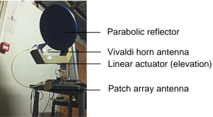
The sensor reading system used here is a Frequency-Modulated Continuous-Wave (FMCW) radar (central frequency: 24 GHz; bandwidth or excursion frequency: Δf=2GHz) with a transmitting parabolic antenna which offers high gain (34.3 dBi) and narrow beamwidth (Δθ=1 degree in azimuth and Δφ=1 degree in elevation). The transmitted signal (power PT=30dBm) or chirp has a linear sawtooth variation of

frequency with time (modulation period TR=18ms). For such

modulation the frequency is tuned linearly as a function of time by using a Voltage-Controlled Oscillator (VCO). The signal backscattered by sensors is received by a 1x4 patch array antenna (beamwidth of the main lobe: 80 degrees in azimuth and 24 degrees in elevation). The received signal is mixed with the front-end transmitted signal and filtered for obtaining I- and Q-channels of the Difference Frequency Signal (DFS). A Fast Fourier Transform with a 2 blocks zero-padding of 512 samples is finally applied to the digitalized DFS (1024 samples per ramp) for deriving the beat frequency spectrum of I- and Q-channels.

Fig. 1 shows the whole system mounted on the experimental setup. The beam steering is performed mechanically. A computer is used to control the movement of the transmitting antenna (and consequently to monitor the antenna beam) and to perform the data acquisition, the signal processing and radar echoes visualization.

The sensor reading system is used to perform the automatized 3D radar scanning for detecting, identifying and remotely reading passive electromagnetic sensors. A sensor is here passive scatterer composed of an antenna (horn antenna; gain: 20dBi) connected to a length of TEM transmission line (a 50-Ω coaxial cable) which is in turn connected to a sensing device, that is, a resistance which depends on the physical quantity of interest. The length of the transmission line is used here for separating in the beat frequency spectrum the

structural scattering mode and the sensing mode (or antenna

scattering mode). Only the radar echo associated to the sensing mode depends on the physical quantity of interest. The structural scattering mode is used here for detecting the sensors.

As shown in Fig. 2 four sensors are located on a 2x2 array. The physical length DCABLE of transmission lines used by

these sensors are: 20cm, 50cm, 75cm and 100cm. With a velocity factor VF of 0.83, these lengths result respectively in

(3)

the following electrical lengths: 24cm, 60cm, 90cm and 120 cm. The distance D between the sensors and the radar is set to 3 meters while the distance DMEAS provided by the radar is

giving by:       + + = D V D D D F CABLE ANT MEAS 2 2 2 1 ₍₁₎

where DANT=30cm denotes the distance between the Vivaldi

horn antenna and the parabolic reflector (see Fig. 1). According to (1), the expected value of DMEAS is 3.75m.

Fig. 1. Transmitting parabolic antenna of the FMCW Radar using a mechanical beam steering

(a) (b)

Fig. 2. Locations of the four passive sensors

The theoretical depth resolution d is given by [6]:

f

c

d

∆

=

2

(2) where c designates the celerity of light in the propagation channel (here an empty corridor of dimensions 1m60 x 2m50 x 20m). In our experimental setup the theoretical depth resolution is then 7.5cm. Angular resolutions in azimuth and elevation are given by the main lobe beamwidth of the transmitting antenna, that is, Δθ=1 degree and Δφ=1 degree. As displayed in Fig. 3, a resolution cell of volume V at the distance D can then be defined by the following relationship: ₎ 2 sin( 2 . . 2 2 3 1 ) ( 3 3

ϕ

θ

∆ ∆               − −       + = D d D d D V (3)

According to (3) the highest density ρ of identifiable/detectable passive EM sensors in the resolution cell V(D) may be derived from:

)

(

1 )

(

D

V

D

=

ρ

. (4) For D=3m one founds ρ(D) = 4860 sensors.m-3_{. However, in}

practice, this theoretical density is reduced by the physical size and RCS of the sensors and, by the beamwidth of the transmitting antenna which may spread the power density backscattered by each sensor through several resolution cells. The maximal detection range is found to be DMAX=50m,

which allows to distinguish two sensors separated by a minimal distance of 88 cm. It corresponds to a density of 15 sensors.m-3_.

Fig. 3. Definition of a resolution cell of volume V at a distance D

Scanning sectors of 12 degrees in azimuth (with 0.5 degree step) and of 13 degrees in elevation (with a 0.72 degree step) are considered. The resistance RL of the sensing device which

loads the sensor transmission line is here 50Ω (match load) or 0Ω (short-circuit). These two values are viewed as the maximum and the minimum resistances taken by the sensing device as the physical quantity of interest varies. For one radar echo acquisition in a given direction in the chosen 3D scanning region, 160 points are recorded which leads to a total of 72000 data points for the entire region.

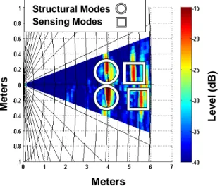
Fig. 4 shows the cut-plane of the resulting radar image for φ=12.9 degrees and for RL=0Ω (the measured echo level is

between -40dB to -15dB). Radar echoes from sensors #3 and #4 can be detected. As expected, the structural scattering mode is found between 3.82m and 4.1m (Note that this mode can be used for identifying the sensor though a specific EM barcode). The sensing modes are apparent when RL=0Ω. The

measured distances between echoes gives 90cm and 128cm, with a ±10 cm error due to the spreading of the echo spot associated to the structural scattering modes. These distances corresponds to the lengths of line used by the sensors #3 and #4, respectively, and could then be used for identifying the two sensors. If sensors are far enough from each other to be distinguished by the radar (a minimum resolution of 5cm at D=3.0m), the distance between these two sensors can be estimated. From elementary geometrical considerations, a Parabolic reflector

Vivaldi horn antenna

Patch array antenna Linear actuator (elevation)

(4)

distance of 24 cm is derived from such measurement with a precision of ±10cm.

A 3D visualization of the radar image can be advantageously used for detecting the echoes due to the sensing modes. In Fig. 5 this visualization is shown for measured echo levels higher than -20dB. The sensing modes are apparent when RL=0Ω (see Fig. 5(b)) and disappear, as

expected, when the sensor antenna is matched (RL=50Ω, see

Fig. 5(a)). From the measurement of the number N of resolution cells for which the echo level P is higher than an arbitrary value PMIN, the echo rate τ of a scanning 3D region

occupying by one sensor is defined by:

T MIN MIN N P P N P ) ( ) ( = >

τ

(5)

where NT denotes the total number of resolution cells in the

scanning region. The echo rate takes its highest value when PMIN is close to the noise level. The contribution of the sensing

mode to this echo rate may then be estimated from the so-called echo rate difference Δτ of a sensor defined by:

∆τ₍_P_MIN₎=τ₂₍_P_MIN₎−τ₁₍_P_MIN₎ (6) where τ1 and τ2 denote the echo rates when RL=0Ω and

RL=50Ω, respectively. When the resistance RL of the sensing

device changes due to the variation of the physical quantity of interest, the Δτ changes accordingly. The value of RL may

then be directly derived from the determination Δτ (note that Δτ is minimal when the resistance RL matches the sensor

antenna while it is maximal when RL=0Ω or when RL is

infinite). For the sake of illustration Fig. 6 displays the measured echo rate difference of sensor #2 as a function of the chosen threshold echo level PMIN (θ sweeps from -3 to 0

degree and, φ from 0 to 6.48 degrees). Δτ reaches its highest value (13%) for PMIN=-40dB and the full-scale dynamic range

is reached when the sensing device resistance is short-circuited. When the resistance RL increases, the echo rate

difference peak decreases. When RL=50Ω the echo rate

difference is 0.

Fig. 4. Radar image in the cut-plane φ=12.9 degrees of a given scanning sector (RL=0Ω).

(a) (b)

Fig. 5. 3D radar image of passive electromagnetic sensors for a minimum echo level of -20 dB: (a) RL=50Ω and (b) RL=0Ω.

Fig. 6. Echo rate difference Δτ as a function of the threshold echo level PMIN of sensor #2.

III. CONCLUSION

The 24GHz FMCW radar scanning technology with a 2GHz bandwidth allows the localization of passive electromagnetic sensors with a depth accuracy of 7.5cm. The 3D visualization of radar images is useful for localizing and identifying passive sensors. A new approach to quantify a load variation of a sensor has been explained by measuring the echo rate difference dynamic range of sensing modes in a volume where is located one single sensor. It has been shown that the full-scale dynamic range of Δτ can reach 13% for a single sensor.

REFERENCES

[1] This reference has been removed because it establishes a direct connection to the authors' names

[6] S.O. Piper, "Receiver frequency resolution for range resolution in homodyne FMCW radar," Telesystems Conference:

Commercial Applications and Dual-Use Technology, 16-17

June 1993, pp.169-173 0 5 10 15 20 -80 -72 -64 -56 -48 -40 -32 -24 -16 -8 0 E CHO RA T E DI F F E RE NCE ( % ) PMIN(dB) FU LL -S C AL E DY NA M IC RA NG E Meters L evel (d B ) Met er s 6m 5m 4m 6m 5m 4m Structural Modes Sensing Modes