HAL Id: hal-02125041
https://hal.archives-ouvertes.fr/hal-02125041
Submitted on 29 Mar 2021
HAL is a multi-disciplinary open access
archive for the deposit and dissemination of
sci-entific research documents, whether they are
pub-lished or not. The documents may come from
teaching and research institutions in France or
abroad, or from public or private research centers.
L’archive ouverte pluridisciplinaire HAL, est
destinée au dépôt et à la diffusion de documents
scientifiques de niveau recherche, publiés ou non,
émanant des établissements d’enseignement et de
recherche français ou étrangers, des laboratoires
publics ou privés.
Johannes Wicht, Thomas Gastine, Lucia D. V. Duarte
To cite this version:
Johannes Wicht, Thomas Gastine, Lucia D. V. Duarte. Dynamo Action in the Steeply Decaying
Conductivity Region of Jupiter-Like Dynamo Models. Journal of Geophysical Research. Planets,
Wiley-Blackwell, 2019, 124 (3), pp.837-863. �10.1029/2018JE005759�. �hal-02125041�
Dynamo Action in the Steeply Decaying Conductivity
Region of Jupiter-Like Dynamo Models
J. Wicht1 , T. Gastine2, and L. D. V. Duarte3
1Max Planck Institute for Solar System Research, Göttingen, Germany,2IPGP, Institut de Physique du Globe de Paris, Sorbonne Paris Cité, Université Paris-Diderot, Paris, France,3College of Engineering, Mathematics and Physical Sciences, University of Exeter, Exeter, UK
Abstract
The Juno mission is delivering spectacular data of Jupiter's magnetic field, while the gravity measurements finally allow constraining the depth of the winds observed at cloud level. However, to which degree the zonal winds contribute to the planet's dynamo action remains an open question. Here we explore numerical dynamo simulations that include a Jupiter-like electrical conductivity profile and successfully model the planet's large-scale field. We concentrate on analyzing the dynamo action in the Steeply Decaying Conductivity Region (SDCR) where the high conductivity in the metallic Hydrogen region drops to the much lower values caused by ionization effects in the very outer envelope of the planet. Our simulations show that the dynamo action in the SDCR is strongly ruled by diffusive effects and is therefore quasi-stationary. The locally induced magnetic field is dominated by the horizontal toroidal field, while the locally induced currents are dominated by the latitudinal component. The simple dynamics can be exploited to yield estimates of surprisingly high quality for both field and currents. These could potentially be exploited to predict the dynamo action of the zonal winds in Jupiter's SDCR but also in other planets.Plain Language Summary
The Juno mission is delivering spectacular data of Jupiter'smagnetic field, while the gravity measurements finally allow constraining the depth of the winds observed at cloud level. However, to which degree the zonal winds contribute to the planet's dynamo action remains an open question. Here we explore numerical simulations of Jupiter's internal dynamics that successfully model the planet's large-scale field. We concentrate on analyzing the dynamo action in the Steeply Decaying Conductivity Region (SDCR) where the high conductivity in the metallic Hydrogen region drops to the much lower values in the outer envelope of the planet. Our simulations show that the dynamo action in the SDCR is strongly ruled by diffusive effects and is therefore rather simple. The simple dynamics can be exploited to yield estimates of surprisingly high quality for both the induced field and the electric currents in the SDCR. These will allow predicting the dynamo action of the zonal winds in Jupiter's SDCR but also in other planets.
1. Introduction
The measurements performed by the Juno mission provide very valuable constraints on the planets interior structure and dynamics. A meaningful interpretation of these data, however, requires a better understand-ing of the underlyunderstand-ing physics, in particular of the dynamo process and the zonal wind dynamics. Ab initio calculations (French et al., 2012) show that the electrical conductivity first increases with depth at a super-exponential rate due to hydrogen ionization. At about 0.90 rJ, where rJis Jupiter's mean radius at the one bar level, hydrogen undergoes a transition from the molecular to a metallic state, and the conductivity increases much more smoothly with depth (see Figure 1).
It is commonly thought that Jupiter's dynamo operates in the deeper metallic region, while the fierce zonal wind system observed on the surface is limited to the molecular outer shell. However, recent numerical simulations show that the interaction between both regions yields complex and interesting dynamics. For example, the zonal winds may drive a secondary dynamo where they reach down to significant enough elec-trical conductivities. Possible features that could reveal such a process are banded structures and large-scale spots at low to middle latitudes (Duarte et al., 2018; Gastine, Wicht, et al., 2014), very similar to what has recently been observed by NASA's Juno mission (Connerney et al., 2018; Moore et al., 2018).
RESEARCH ARTICLE
10.1029/2018JE005759
Key Points:
• Numerical simulations of Jupiter's dynamo are analyzed, concentrating on the outer steeply decaying conductivity region
• We find that the dynamo dynamics in this region is dominated by Ohmic dissipation and can thus be reasonably estimated
• The estimates can be applied to Jupiter or other planets, to reveal the possible dynamo action of zonal winds or other flow contributions
Correspondence to:
J. Wicht, wicht@mps.mpg.de
Citation:
Wicht, J., Gastine, T., & Duarte, L. D. V. (2019). Dynamo action in the steeply decaying conduc-tivity region of Jupiter-like dynamo models. Journal of Geophysical
Research: Planets, 124, 837–863. https://doi.org/10.1029/2018JE005759
Received 10 AUG 2018 Accepted 20 FEB 2019
Accepted article online 24 FEB 2019 Published online 28 MAR 2019
Author Contributions
Conceptualization: J. Wicht Funding Acquisition: J. Wicht Methodology: J. Wicht, T. Gastine, L. D. V. Duarte
Software: J. Wicht, T. Gastine Validation: J. Wicht, T. Gastine, L. D. V. Duarte
Writing - Original Draft: J. Wicht Formal Analysis: J. Wicht Investigation: J. Wicht, T. Gastine, L. D. V. Duarte
Project Administration: J. Wicht Resources: J. Wicht
Supervision: J. Wicht Visualization: J. Wicht
Writing - review & editing: J. Wicht
©2019. American Geophysical Union. All Rights Reserved.
Figure 1. Comparison of the Jupiter interior model by French et al. (2012) and Nettelmann et al. (2012) (black lines) with the model used for the numerical simulations (gray). (a) and (b) show the normalized background density and electrical conductivity, respectively. Dark gray background colors mark the outer 1% that have been neglected in the simulations and the assumed solid core. Note that the core occupies 20% in radius in the numerical models but only 10% in the Jupiter model (black density profile). Medium gray highlights the Steeply Decaying Conductivity Region.
One of the main Juno objectives is to determine the depth of the fierce zonal winds observed on the planet's surface. Since the wind dynamics is tied to density variations, the gravity signal can help to constrain their depth. A recent analysis by Kaspi et al. (2018), based on the equatorially antisymmetric gravity moments J3 to J9measured by the Juno mission (Iess et al., 2018), concludes that the wind speed must be significantly reduced at about 3,000 km depth, which corresponds to about 0.96 rJ. This conclusion is supported by new interior models based on Juno data (Guillot et al., 2018). Kong et al. (2018), however, point out that the problem is nonunique and that the gravity signal could also be explained by deeper reaching but weaker zonal flows that may not reflect zonal jets observed at cloud level. Another hint on the depth of the zonal winds comes from the width of the prograde equatorial jet. Numerical simulations show a dependence on the depth of the spherical shell the winds live in and suggest a lower boundary at about 0.95 rJ(Gastine, Heimpel, & Wicht, 2014).
Other estimates of the wind depth rely on magnetic effects. Liu et al. (2008) concluded that winds cannot reach deeper than 0.96 rJ with undiminished speed since the Ohmic heating produced by the zonal-wind-induced electric currents would otherwise exceed the heat emitted from the planet's interior. Ridley and Holme (2016) argue that the secular variation of the large-scale field, deduced from pre-Juno measurements, is so small that the zonal winds cannot contribute. The winds are thus unlikely to penetrate
Journal of Geophysical Research: Planets
10.1029/2018JE005759
deeper than about 0.96 rJwhere the magnetic Reynolds number exceeds unity (Cao & Stevenson, 2017; Liu et al., 2008).
Classically, the magnetic Reynolds number attempts to quantify the ratio of magnetic induction to Ohmic dissipation in the induction equation
𝜕B
𝜕t = ∇ × (U × B) − ∇ × (𝜆∇ × B) , (1)
where 𝜆 = 1∕(𝜇𝜎) is the magnetic diffusivity with 𝜎 the electrical conductivity and 𝜇 the magnetic permeability. The Ohmic dissipation term can be separated into two parts:
∇ × (𝜆∇ × B) = −𝜆∇2B + 𝜆
d𝜆̂r × (∇ × B) , (2)
where the second part depends on the magnetic diffusivity scale height d𝜆 = 𝜆∕(𝜕𝜆∕𝜕r). The standard magnetic Reynolds number,
Rm = Ud
𝜆 , (3)
ignores the second term. Here d is a reference length scale and U a typical flow velocity. Liu et al. (2008) argue that the appropriate definition for the region where the electrical conductivity decays steeply should be based on the second term in equation (2) and must therefore include the diffusivity scale height d𝜆:
Rm(1)= Ud𝜆
𝜆 . (4)
In Jupiter, Rm(1)would characterize a Steeply Decaying Conductivity Region (SDCR) that roughly coincides with the molecular outer envelope where ionization effects determine the electrical conductivity.
For a self-consistent dynamo to operate, the overall field production has to overcome diffusion. The mean global magnetic Reynolds number for the whole dynamo region should thus exceed a critical value Rmc = 1. Since the definition of Rm ignores many complexities of the dynamo process, the exact critical value is always higher and can only be determined by experiments. Christensen and Aubert (2006) explore a suite of Boussinesq dynamo simulations with rigid flow boundary conditions and constant conductivity and find self-consistent dynamo action when the Root Mean Square (rms) magnetic Reynolds number exceeds Rmc≈ 50.
The radius rDwhere the magnetic Reynolds number exceeds Rmcindicates the “top of the dynamo region” that could potentially host self-consistent dynamo action. Gastine, Wicht, et al. (2014) and Duarte et al. (2018) use Rmc ≈ 50in combination with the classical Rm definition (3) and show that their numer-ical simulations produce Jupiter-like magnetic fields when rD ≥ 0.9 rJ. Extrapolating their findings to Jupiter conditions, using the conductivity profile suggested by French et al. (2012) and estimates for the rms nonaxisymmetric flow velocity, suggests that rD≈0.95 rJ(Duarte et al., 2018).
There are several reasons why these considerations are problematic. For one, self-consistent dynamo action and the related critical magnetic Reynolds number are defined in a mean sense for the whole dynamo region. The local dynamo mechanism at any given radius, however, also includes the modification of the field produced elsewhere. Another fundamental problem is that the magnetic Reynolds number actually ceases to provide a decent proxy for the ratio of induction to diffusion in the SDCR where the magnetic field approaches a diffusion-less potential field.
A more useful definition of the top of the dynamo region would be the depth where the Locally Induced Field (LIF) becomes a significant fraction of the total field. Cao and Stevenson (2017) suggest that Rm(1)takes on a different role in the SDCR and may allow to quantify the ratio of the LIF ̂B to the background field ̃B.
Using a simplified mean field dynamo model, they conclude that ̂B could reach 1% of the background field
in the SDCR.
In this article we closely analyze the dynamo action in the SDCR for two different numerical dynamo simula-tions that both yield Jupiter-like large-scale magnetic fields. After presenting the numerical dynamo model in section 2, we analyze the simulation results in section 3. Section 4 is devoted to estimates for the locally induced electric currents and fields that allow predicting the dynamo action in the SDCR of planets. The paper closes with a discussion and conclusions in section 5.
2. Numerical Dynamo Model
2.1. Fundamental EquationsThe numerical simulations were performed with the magneto-hydrodynamics code MagIC, which is freely available on GitHub (https://github.com/magic-sph/magic). MagIC solves for small disturbances around an adiabatic, hydrostatic background state that only depends on radius. Using the anelastic approximation for the Navier-Stokes equation allows incorporating a background density profile while filtering out fast sound waves.
The background state is based on the Jupiter model by French et al. (2012) and Nettelmann et al. (2012), who use ab initio simulations to determine the equation of states for Hydrogen and Helium and to calculate the transport properties. Figure 1 shows the normalized density profile ̃𝜌(r) and the normalized electrical conductivity profilẽ𝜎(r) along with the respective profiles that have been assumed in the simulations. The transition to a metallic hydrogen state takes place at about 0.9 rJ. Jupiter's SDCR thus roughly occupies the outer 10% in radius where the conductivity decays increasingly rapidly with radius, eventually reaching superexponential rates.
The numerical models disregard the outer 1% in radius where the density gradient is steepest and thus very difficult to resolve numerically. The conductivity profile used in the simulations is a combination of a polynomial branch 𝜎 = 𝜎i− (𝜎i−𝜎m) ( r − ri rm−ri )a for r< rm, (5)
and an exponential branch
𝜎 = 𝜎mexp ( a r − rm rm−ri 𝜎m−𝜎i 𝜎m ) for r≥ rm. (6)
Here𝜎iis the reference conductivity at the bottom boundary ri, a is the exponential decay rate, and rmthe transition radius where both branches meet with𝜎(rm) =𝜎m. The profiles in the dynamo simulations G14 and D18 use rr = ri = 0.2 rJ, a = 13, rm = 0.9, and 𝜎m = 𝜎r∕5.
While the ab initio simulations suggest that the conductivity already slowly decreases in the metallic region, the numerical simulations assume a constant value here. This keeps the magnetic Reynolds number at amplitudes that allow for dynamo action throughout this region (Duarte et al., 2018). The conductivity also decreases slower in the outer region than suggested by French et al. (2012) to ease the numerical calcula-tions. The total conductivity contrasts are thus smaller than in the Jupiter model but still reach about four orders of magnitude. In the numerical simulations, the SDCR is roughly identical to the exponential branch. The mathematical formulation of the problem has been extensively discussed elsewhere (Jones et al., 2011; Wicht et al., 2018). Detailed information can also be found in the online MagIC manual (http://magic-sph.github.io/). Here we only briefly introduce the essential equations.
MagIC solves the nondimensional Navier-Stokes equation Ẽ𝜌dU dt = −̃𝜌 ∇ ( p ̃𝜌 ) +2̃𝜌 U × ̂z −Ra ′E PrDi ̃𝜌 𝜕 ̃T 𝜕r ŝr + 1 Pmi (∇ ×B) × B + E ̃𝜌 Fv, (7)
the heat equation
̃𝜌 ̃Tds dt = 1 Pr∇ · ( 𝜌 ̃T ∇s)+PrDi Ra′ ( q𝜈+ 1 Pm2iEqJ ) +qs, (8)
the induction equation
𝜕B
𝜕t = ∇ × (U × B) − 1
Pmi∇ × ( ̃𝜆∇ × B), (9)
the continuity equation
Journal of Geophysical Research: Planets
10.1029/2018JE005759
and the solonoidal condition for the magnetic field
∇ ·B = 0. (11)
Here p is a modified pressure that includes centrifugal effects and accounts for disturbances in the gravity potential. Buoyancy variations are formulated in terms of the specific entropy s. Using the gradient of the normalized background temperature ̃Tin the buoyancy term guarantees a consistent background gravity (Wicht et al., 2018). The three volumetric heating terms in equation (8) are viscous heating q𝜈, Joule or Ohmic heating qJ, and secular cooling qs(Jones, 2014; Wicht et al., 2018).
The dimensionless parameters ruling the system are the Ekman number
E = 𝜈
Ωd2, (12)
the modified Rayleigh number
Ra′=𝛼õgod3̃To 𝜈𝜅S ss cp =Ra ss cp, (13)
the Prandtl number
Pr = 𝜈 𝜅S
, (14)
and the inner-boundary magnetic Prandtl number Pmi= 𝜈𝜆
i
. (15)
Here𝜈 is the (homogeneous) kinematic viscosity, 𝛺 the rotation rate, 𝛼othe outer-boundary thermal expan-sivity, ̃gothe outer-boundary gravity, ̃Tothe outer boundary background temperature, d = ro − rithe shell thickness,𝜅S the entropy diffusivity, ss the entropy scale, cp the heat capacity,𝜆i = 1∕(𝜇o𝜎i) the inner-boundary magnetic diffusivity, ̂r the radial unit vector, and ̂z the unit vector in the direction of the rotation axis. The aspect ratio, another dimensionless parameter, has been fixed to ri∕ro = 0.2.
The modified Rayleigh number Ra′is the product of the classical Rayleigh number Ra and the dimensionless entropy scale ss∕cp. The dissipation number,
Di = d ̃To (𝜕 ̃T o 𝜕r ) = d𝛼õgo cp , (16)
is defined by the background temperature profile ̃T.
The equations have been nondimensionalized by using the imposed entropy difference as entropy scale ss, das a length scale, the viscous diffusion time d2∕𝜈 as a time scale, and√Ω𝜇0𝜆ĩ𝜌oas a magnetic scale, where ̃𝜌ois the outer-boundary reference density. We use entropy rather than temperature diffusion in the heat equation, which considerably simplifies the system (Braginsky & Roberts, 1995; Lantz & Fan, 1999). In the above formulation, the dimensionless profiles ̃𝜌, ̃T, and ̃𝜆 carry the information on the radial dependence of the background state.
2.2. Poloidal/Toroidal Decomposition
We use the common representation of the divergence free magnetic field by a poloidal and a toroidal contribution,
B = B(P)+B(T)= ∇ × ∇ ×̂r b(P)+ ∇ ×̂r b(T), (17) where b(P)is the poloidal and b(T)the toroidal scalar potential. The respective decomposition for the electric current density j reads
Table 1
Parameters of the Numerical Dynamo Simulations Explored Here
Name E Ra Pm Pr
D18 10−4 6 × 10⁷ 2 0.1
G14 10−5 5 × 10⁹ 0.6 1
Note. Both simulations use background density and temperature models very close to those suggested by Nettelmann et al. (2012) and the electrical conductivity profile illustrated in Figure 1.
where i(P)denotes the poloidal and i(T)the toroidal potential. Simple vector calculus yields
j = −∇2 Hi
(P) ̂r + ∇
H𝜕r𝜕 i(P)+ ∇ ×̂r i(T), (19)
where ∇His the horizontal component of the nabla operator. The toroidal contribution obviously has no radial component. Radial derivatives appear only in the horizontal poloidal current density, which therefore dominates in the SDCR, as we will show below.
Ampere's law, ∇ × B = 𝜇j, connects the poloidal (toroidal) magnetic field to the toroidal (poloidal) current density. Its radial component establishes a connection between toroidal current density and toroidal field potentials:
𝜇 𝑗r= −𝜇∇2Hi
(P)=̂r · (∇ × B) = −∇2 Hb
(T). (20)
The toroidal field at a given radius is thus determined by the radial currents flowing through the respective radial shell.
The radial component of the curl of Ampere's law provides a relation between the toroidal current and poloidal magnetic field potentials:
𝜇 ̂r ·(∇ ×j)= −𝜇 ∇2Hi(T)=̂r · (∇ × ∇ × B) (21) = −(1 r2 𝜕 𝜕rr2𝜕r𝜕 + 2 r2− ∇ 2 H ) Br (22) = ∇2H [(𝜕 𝜕r )2 + ∇2H ] b(P). (23) 2.3. Selected Simulations
We concentrate on closely analyzing two quite different dynamo simulations that both reproduce Jupiter's large-scale field (Duarte et al., 2018). Model G14 has been introduced by Gastine, Wicht, et al. (2014), while model D18 is listed as model number 20 in Duarte et al. (2018); Table 1 compares their parame-ters. Both dynamos share the background pressure, temperature, density, and electrical conductivity models (see Figure 1 for the latter two), use stress-free outer but rigid inner-boundary conditions, employ constant entropy boundary conditions, and are driven by heat coming in through the lower boundary. Model D18 uses a larger Ekman and larger magnetic Prandtl number. The Prandtl number is one in G14 but only 0.1 in D18, which yields a smaller-scale field in the latter simulation (Duarte et al., 2018).
Figure 2 compares the radial surface fields for the two snapshots which we will continue to analyze through-out the paper with the recent Jupiter field model JRM09 by Connerney et al. (2018), demonstrating that the numerical simulations at least capture Jupiter's large-scale field. A closer comparison with the older field model VIP4 (Connerney et al., 1998) can be found in Gastine, Wicht, et al. (2014) and Duarte et al. (2018). Figure 3 illustrates the flow structure for both dynamos. They share the fact that the zonal flows (left panels) show a pronounced equatorial jet but not the multitude middle to high latitude jets observed in Jupiter's or Saturn's cloud structure. These jets seem incompatible with dipole-dominated magnetic fields in the
numer-Journal of Geophysical Research: Planets
10.1029/2018JE005759
Figure 2. Comparison of the radial field in the recent Jupiter field model JRM09 (Connerney et al., 2018), plotted on a spherical surface with radius rJ, with the radial surface fields in the two snapshots of the dynamo D18 and G14 closely explored here. G14 has been rescaled to mT with the power-based scaling (Duarte et al., 2018; Gastine, Wicht, et al., 2014). Because this would yield a too strong field for D18, we have scaled the field strength of the snapshot to JRM09 values for illustration purposes. Hammer projection shown.
ical simulations (Duarte et al., 2013; Gastine et al., 2012). The rms nonaxisymmetric flow amplitude (right panels in Figure 3) increases with radius because of the decreasing density (Gastine & Wicht, 2012). 2.4. Magnetic Reynolds Numbers
As already discussed in section 1, the strong decrease in the electrical conductivity in the SDCR requires a modification of the classical magnetic Reynolds number. In addition to profiles following the classical definition, Rm = ⟨U⟩ d 𝜆 , (24) we will use Rm(1)= ⟨U⟩ d𝜆 𝜆 , (25) and Rm(2)= ⟨U⟩ d 2 𝜆 𝜆 d , (26)
Figure 3. Zonal flows (left panels) and rms nonaxisymmetric flows (right panels) for dynamo D18 and dynamo G14 snapshots. Rossby number scales, Ro =U∕(d𝛺), have been used here.
where d𝜆 = 𝜆∕(𝜕𝜆∕𝜕r) is the magnetic diffusivity scale height. Angular brackets generally denote spherical rms values, ⟨𝑓(r)⟩ = ( 1 4𝜋 ∫ 1 −1dx ∫ 2𝜋 0 d𝜙𝑓2 )1∕2 , (27)
with𝜙 being longitude, 𝜃 colatitude, and x = cos(𝜃). ⟨U⟩ thus indicates the rms velocity at a given radius. Figure 4 compares the different magnetic Reynolds number profiles for the D18 and G14 snapshots, sepa-rating zonal flow and nonaxisymmetric flow contributions. Axisymmetric latitudinal and radial flows are typically much weaker and have thus been neglected here. While zonal and nonaxisymmetric flows have comparable amplitudes in the SDCR of dynamo D18, the zonal flows are somewhat more pronounced in model G14 because of the smaller Ekman number. In the exponential branch of the conductivity profiles, the
Journal of Geophysical Research: Planets
10.1029/2018JE005759
Figure 4. Radial profiles of the three different magnetic Reynolds numbers for the selected snapshots of dynamo models D18 and G14. Vertical lines mark the radii where Rm(1)= 1 (solid), Rm(1)= 5 (dashed), and Rm(2)= 1 (dotted) for the total rms flow. A rescaled electrical conductivity profile𝜎(r)(thick gray) has been include in order to
demonstrates that it dominates the radial gradients in the Steeply Decaying Conductivity Region (medium gray background).
diffusivity scale height assumes a constant value of d𝜆 = 0.168, which explains why the different Rm profiles are parallel in this region (see Figure 4).
3. Dynamo Action in the SDCR
Ohm's law,j =𝜎 (U × B + E) , (28)
states that the electric currents are driven by induction or by an electric field E. Since both effects scale with𝜎, the current density j has to decay in the SDCR. Figure 5 illustrates the radial decay of the different current density components for the selected snapshots in dynamos D18 (top panel) and G14 (bottom panel). The poloidal current (solid lines), more specifically its latitudinal component (solid blue), dominates in the SDCR. The rms poloidal current is at least two times larger than the toroidal current in model D18 and about five times larger than its toroidal counterpart in model G14. The likely reason for the larger difference is the stronger zonal flow in the latter simulation. Radial currents (solid black) are effectively blocked by the conductivity gradient and are thus generally small.
Figure 5. Radial profiles of different rms current contributions. Light gray background colors indicate where the conductivity is smaller than 50% of its reference values at ri; medium gray highlights the Steeply Decaying Conductivity Region where the conductivity decays exponentially. Top and bottom panels show the selected snapshots for dynamos D18 and G14, respectively. Vertical lines mark the radii where Rm(1)= 1 (solid) and Rm(1)= 5 (dashed). A rescaled electrical conductivity profile𝜎(r)has been included to demonstrate that it determines the radial gradient. Dimensionless quantities shown.
As expected, the decrease of the rms current density in the SDCR is mostly dictated by the electrical conduc-tivity profile (thick gray line in Figure 5) with local induction effects providing some moderation. Below the SDCR, the current increases much more smoothly with depth and never exceeds twice the value reached at the bottom of the SDCR. The transition to more classical dynamo action seems to kick in somewhere between Rm(1)= 1 (solid vertical line in Figure 5) and Rm(1)= 5 (dashed vertical line).
In the simulations we assume that the region r > rois electrically insulating. The current-free conditions, gradually approached with radius in the SDCR, are therefore abruptly enforced at ro. Figure 5 illustrates that this leads to a thin boundary layer where the simple dependence on𝜎 breaks down. Since the currents are rather small in this very outer region, it also becomes increasingly difficult to calculate reliable values based on the single precision snapshots stored during the simulations.
Of particular interest is the fraction of the total field produced by the currents flowing in the SDCR. The toroidal LIF is directly given by the local poloidal currents (see equation (20)). The local poloidal field, however, is in principle produced by all the electric currents in the system. To quantify the LIF, we analyze the field ̂B(r) that is induced by the currents flowing in the region above r. Since the currents and thus ̂B(r)
Journal of Geophysical Research: Planets
10.1029/2018JE005759
Figure 6. Comparison of the rms values from approximations (30) and (31) of the Locally Induced Field with𝛿Band the true toroidal field. Vertical lines mark the radii where Rm(1)= 1 (solid), Rm(1)= 5 (dashed), and Rm(2)= 1 (dotted). A rescaled electrical conductivity profile𝜎(r)has been included to demonstrate that it determines the radial gradient.
steeply decrease with radius, Ampere's law simplifies to 𝜕 ̂BH
𝜕r ≈ −𝜇 ̂r × jH, (29)
where the index H refers to the horizontal components. Integration in radius yields ̂BH(r) ≈𝜇 ̂r × ∫
ro
r dr′j
H(r′). (30)
Similarly, an integration of equation (21) provides an approximation for the radial LIF: ̂Br(r) ≈ −𝜇 ∫ ro r dr′ ∫ ro r′ dr′′ ̂r ·[∇′′×j(T)(r′′ )]. (31)
We have assumed here that ̂B and its radial derivative vanish at the outer boundary.
As long as the local currents are small, the downward continuation of the surface field, according to the characteristic radial dependence of a potential field, provides a decent approximation of the total poloidal field:
Figure 7. Rms values of different magnetic field contributions. The downward continued potential field̃B(dashed lines) only starts to deviate more significantly from the poloidal fieldB(P)(solid lines) below the radius where Rm(1)= 1 (vertical solid line). See caption of Figure 6 for more explanations.
̃B𝓁(r) =( ro r
)𝓁+2
B𝓁(ro) ≈B(P)(r). (32)
We will thus use ̃B(r) as a proxy for the background field in the SDCR dynamo process.
The difference,
𝛿B = B(P)− ̃B, (33)
provides a measure for the additional poloidal field produced by the local dynamo mechanism. Both𝛿B and ̂B vanish at the outer boundary and decay radially with the electrical conductivity. Figure 6 compares rms profiles of the different𝛿B and toroidal field contributions with those provided by approximations (30) and (31). Using the toroidal or poloidal current densities allows separating the poloidal and toroidal LIF, respec-tively. The close agreements confirm the high quality of the approximations. Pearson correlation coefficients are close to 1 for the toroidal horizontal components, above 0.95 for the poloidal horizontal components, and above 0.9 for the radial component in the SDCR of dynamos G14 and D18. Figure 6 demonstrates that the azimuthal toroidal field (dashed red) dominates the other LIF components, likely due to the𝛺 effects provided by the shearing action of the zonal winds.
Figure 7 compares the rms values of the LIF to the total poloidal field B(P)and the downward continued field ̃B. The latter stops proving a reasonable approximation of the background field somewhere between the
Journal of Geophysical Research: Planets
10.1029/2018JE005759
Figure 8. Radial (solid) and horizontal (dashed) rms length scales of different field contributions. See caption of Figure 6 and the main text for more explanations.
radii where Rm(1) = 1(solid vertical line) and Rm(1) = 5(dashed vertical line). The azimuthal component of the toroidal field reaches the respective background field component where Rm(1)≈1. We come back to discussing this issue in section 4.
Radial and horizontal magnetic field length scales, based on the respective derivatives of the field potentials, are illustrated in Figure 8. For example, the radial scales of the poloidal field are estimated via
dr(B(p)) = ⟨b(P)⟩
⟨𝜕b(P)∕𝜕r⟩. (34)
Horizontal scales have been calculated using the square root of⟨∇2
Hb⟩. Between r = 0.90 roand r = 0.97 ro, the radial scale of ̂B and of the toroidal field is indeed very similar to the diffusive scale height d𝜆, which confirms that the conductivity profile determines the radial gradient of the LIF. The horizontal length scales of both LIF contributions are significantly smaller than the respective scales of the total field (or the potential field) but still an order of magnitude larger than the radial scales.
The separate evolution equations for the toroidal and poloidal field potentials solved by MagIC are the radial component of the induction equation (Christensen & Wicht, 2007),
∇2Hb.(P)= −̂r · [∇ × (U × B)] + 𝜆 ∇2H[(𝜕 𝜕r )2 + ∇2H ] b(P), (35)
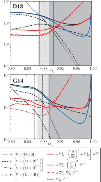
Figure 9. Horizontally averaged rms values of the different contributions to the poloidal induction equation for the snapshots in dynamos D18 (top) and G14 (bottom). See caption of Figure 6 for more explanations.
and the radial component of its curl,
∇2Hb.(T)= −̂r · [∇ × ∇ × (U × B)] + 𝜆 ∇2H [ (𝜕 𝜕r )2 + ∇2H+ 1 d𝜆 𝜕 𝜕r ] b(T). (36)
Only the toroidal field equation directly includes the magnetic diffusivity scale height.
Figure 9 shows radial profiles of the rms values of the different contributions in the poloidal evolution equation for the D18 and G14 snapshots. Very close to the outer boundary beyond r ≈ 0.98 ro, the use of single precision snapshot data limits the quality of the second radial derivative required for the diffusive contributions. The balance should thus not be interpreted in this region.
We have separated the diffusive term into two contributions involving radial (red dashed line) and only horizontal (red dotted) derivatives. Both increase with𝜆 toward the outer boundary but also progressively cancel each other since the field approaches a potential field. What remains is the diffusive term for the LIF (red solid), which is mostly balanced by the induction term (black solid). Consequently, magnetic field variations (blue) become comparatively small in the highly diffusive SDCR, and the dynamics becomes quasi-stationary.
Journal of Geophysical Research: Planets
10.1029/2018JE005759
Figure 10. Horizontally averaged rms values of the different contributions to the toroidal induction equation for the snapshots in dynamos D18 (top) and G14 (bottom). See caption of Figure 6 for more explanations.
Figure 9 also illustrates that induction due to zonal flows (black dashed-dotted) is sizable for the poloidal field evolution. This describes pure advection of the background field ̃B. Induction due to flow acting
on the toroidal field (black dashed) or the poloidal LIF (black dotted), on the other hand, remain minor contributions in the SDCR.
For the toroidal field evolution, depicted in Figure 10, time variations are even less important in the SDCR than for the poloidal counterpart. The two dominant diffusive terms that involve radial derivatives (red dashed and dash-dotted lines) cancel to a high degree. This is simply a consequence of the fact that the toroidal field decreases with𝜎 so that
𝜕
𝜕r b(T)≈ − b(T)
d𝜆 . (37)
Zonal flows clearly dominate the toroidal field induction, in particular for dynamo G14.
Vertical lines in Figures 9 and 10 mark where the magnetic Reynolds number Rm(1)exceeds one (solid) and five (dashed). The assumption of quasi-stationary dynamics seems to be limited to the region Rm(1)≤ 1.
As we will discuss below, Rm(2)roughly quantifies the ratio of radial field induction to diffusion in the SDCR. Where Rm(2)= 1, indicated by the dotted vertical line in Figure 9, we would thus expect comparable rms values of diffusion (red line) and induction (black line). This is not the case, however, since the respective radius already lies below the SDCR.
4. Estimating the Dynamo Action
The analysis of dynamo simulations has shown that the dynamo action in the SDCR is dominated by diffu-sive effects and thus obeys a quasi-stationary dynamics. In this section, we exploit this simplicity and derive expressions that could be used to estimate the dynamo action in the SDCR of planets.
4.1. Estimating the Electric Currents
The decent balance between diffusion and induction in the dynamo equation suggests ∇ × j
𝜎 ≈ ∇ × (
U × ̃B). (38)
When using the fact that the horizontal current components dominate in the SDCR, this leads to the radial integral estimate𝓙Hused by Liu et al. (2008):
jH≈𝓙H(r) = 𝜎 r [ r′ 𝜎jH ] ro + 𝜎 r ̂r × ∫ ro r dr′r′[∇ ×(U × ̃B)] H. (39)
The square brackets with index roindicate a value taken at the outer boundary. We will generally assume that the current vanishes at ro.
A simpler estimate can be based on Ohm's law. Since the dynamics in the SDCR is to a good degree quasi-stationary, the electric field contributions due to magnetic field variations, expressed by the Maxwell-Faraday law𝜕B∕𝜕t = −∇ × E, are small. Ohm's law thus reduces to
j =𝜎 (U × B − ∇V) , (40)
where V is the electric potential.
Taking the radial component of the curl of Ohm's laws shows that the electric potential does not contribute to the toroidal current density:
∇2Hi(T)≈ −𝜎 ̂r · ∇ ×(U × ̃B). (41)
Solving this differential equation in spectral space yields i(T)𝓁 =𝜎 r
2 𝓁(𝓁 + 1) ̂r ·
[
∇ ×(U × ̃B)]𝓁, (42)
where the subindex𝓁 denotes contributions of spherical harmonic order 𝓁. We will formally use the notation i(T)≈ −𝜎 ∇−2
H ̂r · ∇ × (
U × ̃B), (43)
in the following, where ∇−2
H denotes the inverse of the horizontal Laplace operator. The toroidal current density can then be estimated according to equation (18):
j(T)≈ −𝜎∇ × ̂r[∇−2 H ̂r · ∇ ×
(
U × ̃B)]. (44)
Ignoring the horizontal derivatives and the cross product yields the simpler approximation ⟨j(T)⟩ ≈ Rm⟨ ̃B⟩
𝜇d (45)
for the rms values of the toroidal current density. In order to quantify the quality of the two estimates, we compare the ratio of the estimated to the true rms values at each radial level. The respective ratios read
R𝑗T=𝜎 ⟨∇ × ̂r [ ∇−2 H ̂r · ∇ × ( U × ̃B)]⟩ ⟨j(T)⟩ , (46)
Journal of Geophysical Research: Planets
10.1029/2018JE005759
for expression (44) and
R′
𝑗T=Rm 𝜇d⟨j⟨ ̃B⟩(T)⟩, (47)
for the simplified version (45). Figure 11a demonstrates that equation (44) does a good job in capturing the rms of the toroidal currents in the SDCR with deviations of less than 50%. Below the SDCR, the approx-imation tends to overestimate the true current amplitude but nevertheless remains acceptable down to about 0.85 ro. The simplified version (45), however, severely overestimates the toroidal current density in the SDCR, indicating that the horizontal derivatives cannot be ignored in equation (44).
Perhaps more relevant is an estimate for the larger poloidal current contribution. A tempting approach is to ignore the electric potential altogether and simply assume
j ≈𝜎(U × ̃B), (48)
which we refer to as the simplified Ohm's law or Ohm's law for a fast moving conductor in the following. Such an approach seems at least justified for the dominant current component, that is, for the latitudinal poloidal current that is mostly induced by fast azimuthal flows that render the electric potential contribution secondary.
For estimating the rms electrical current, we can rely on the dominant poloidal components. When ignoring the cross product, equation (48) suggests
⟨j⟩ ≈ Rm ⟨ ̃B⟩𝜇d. (49)
To quantify the quality of this estimate, we calculate the ratio R𝑗=Rm ⟨ ̃B⟩
𝜇d⟨j⟩, (50)
which can be compared to the respective ratio for the integral estimate (39): R′
𝑗= ⟨𝓙H⟩
⟨j⟩ . (51)
Figure 11b illustrates that the simplified Ohm's law yields a good approximation which overestimate the current density by typically less than a factor two in the SDCR. We have used magnetic Reynolds numbers based on the zonal flows in Figure 11b, which provide slightly better estimates, in particular for model G14. The integral estimate largely captures the right order of magnitude at the bottom of the SDCR where the currents are stronger, but generally seems of lower quality.
The simplified Ohm's law severely overestimates the weaker radial currents, which is likely related to a stronger electric potential contribution boosted by the radial derivative𝜕V∕𝜕r. An improved estimate can be calculated from the poloidal current potential derived from the estimate for the horizontal components. Taking the horizontal divergence of equation (48) yields
∇2H 𝜕
𝜕ri(P)≈ − 𝜕𝜕r𝑗r≈𝜎 ∇H· (U × B)H. (52)
This suggests the integral estimate
𝑗r(r) ≈r(r) = ∫ ro
r
dr′𝜎 ∇
H· (U × B)H. (53)
Since the gradient in𝜎 dominates the integral, the expression can be simplified to 𝑗r≈ −d𝜆𝜎 ∇H·
(
U × ̃B)H. (54)
Figure 11. Ratio of estimates and true rms electric current densities. The results have been averaged over 14 snapshots for dynamo D18 and 10 snapshots for dynamo G14. Transparent background stripes with a width of two standard deviations illustrate the variability. (a) shows ratios (46) (solid lines) and (47) (dotted lines) for the toroidal currents density. (b) shows ratio (50) for the total rms current density based on Ohm's law (solid lines) and the respective ratio (51) for the integral estimate (dotted lines). Here we have used magnetic Reynolds numbers based on the zonal flows. (c) compares ratios (56) (solid lines) and (57) (dotted lines) for the radial current densities. Solid (dashed) vertical lines mark where Rm(1)= 1 (Rm(1)= 5). The medium gray background highlights the Steeply Decaying Conductivity Region where the conductivity decreases exponentially, while light gray marks the region where the conductivity is smaller than 50% of the inner-boundary reference value.
Journal of Geophysical Research: Planets
10.1029/2018JE005759
Figure 12. Pearson correlation coefficients between individual current density components and two different estimates. Solid lines refer to the estimates based on the simplified Ohm's law (48), while dotted lines refer to the integral expression (39) for the horizontal and (54) for the radial component. See caption of Figure 11 for more explanations.
⟨𝑗r⟩ ≈ Rm(1) ⟨ ̃B⟩
𝜇d. (55)
The quality ratio based on equation (54) reads
R𝑗r=d𝜆𝜎⟨∇H· (
U × ̃B)H⟩
⟨𝑗r⟩
, (56)
while the simplified version (55) yields R′
𝑗r=Rm(1) 𝜇d⟨j⟩⟨ ̃B⟩ . (57)
Figure 11c demonstrates that the simplified version severely underestimates the radial current density by at least an order a magnitude in the SDCR, while the more complex expression (54) deviates by not more than about 30% from the true values. This confirms that the horizontal derivatives cannot be ignored.
Figure 11 suggests that the higher quality estimates remain reliable throughout the whole SDCR. The assumption of a dominant background potential field but also of the quasi-stationary dynamo action roughly holds for Rm(1) ≤ 1. The radii where Rm(1) = 1and Rm(1) = 5have been marked by vertical lines in Figure 11. Some estimates provide acceptable values down to the latter radius, and the higher quality estimates of the toroidal and total current density yield acceptable values for even deeper radii.
Figure 13. Comparison of (a)𝜇j𝜃with (b) estimate Pm(U × ̃B)𝜃at r= 0.94rofor the snapshot of dynamo G14. Dimensionless values shown.
To assess whether the estimates of the individual current density components not only capture the rms amplitudes but also the structure, we calculate the Pearson correlation coefficients for each radius. For example, for the total latitudinal current density, the coefficient reads
C(𝑗𝜃, 𝜎(U × B)𝜃) = ( 𝑗𝜃−𝑗𝜃 ) ( [U × B]𝜃− [U × B]𝜃) [( 𝑗𝜃−𝑗𝜃 )2 ( [U × B]𝜃− [U × B]𝜃) 2]1∕2 , (58)
where the overbars refer to an average over a spherical surface. The results, shown in Figure 12, demonstrate that𝜎U × ̃B not only provides a better rms estimate but also a better local estimate than the integral esti-mate𝓙Hfor the horizontal current components. Particularly high correlations are reached for the toroidal and the total latitudinal current densities where the simplified Ohm's law can reasonably be applied. The inferior correlations for the azimuthal current density point toward a stronger contribution from the elec-tric potential. For the radial component, equation (53) provides a very decent local estimate with Pearson coefficients up to 0.85 for G14. Figure 13 illustrates the close agreement for the latitudinal current density in model G14 at r = 0.94 ro. The stronger dynamo action at low to middle latitudes caused by the shear in the zonal flow is clearly apparent.
4.2. Estimating the LIF
Using the current provided by the simplified Ohm's law (30) for the horizontal field yields the integral estimate𝓑Ofor the horizontal LIF:
̂BH≈ ∫ ro r dr ̂r × ( U × ̃B) 𝜆 . (59)
This can be further simplified to
̂BH≈ d𝜆
𝜆 ̂r × (
U × ̃B), (60)
since the conductivity profile dominates the radial dependence. The expression suggests a rather simple estimate for the rms value of the LIF, which is dominated by the toroidal field:
Journal of Geophysical Research: Planets
10.1029/2018JE005759
⟨ ̂B⟩ ≈ Rm(1)⟨ ̃B⟩. (61)
For estimating the radial poloidal field, we rely on equation (31): ̂Br≈ −𝜇 ∫ ro r dr′ ∫ ro r′ dr′′𝜎 ̂r ·(∇′′×[U × ̃B])≈ −d 2 𝜆 𝜆 ̂r · ∇ × ( U × ̃B). (62) This is equivalent to assuming a balance between induction and diffusion in the induction equation (35) and approximating the latter term with𝜆∕d2
𝜆̂Br.
Ignoring the curl and cross product suggests that the rms value of the radial LIF can be estimated via
⟨ ̂Br⟩ ≈ Rm(2)⟨ ̃B⟩. (63)
Taking the radial derivative of equation (62) yields a differential equation for the horizontal poloidal LIF: 𝜕 𝜕r̂Br≈ −∇2H𝜕r𝜕 ̂b (P)= −∇ ĤB (P) H ≈ d𝜆 𝜆 ̂r · ∇ × ( U × ̃B). (64)
We solve this equation by taking the horizontal derivatives in spectral space and formally write the result as ̂B(P) H ≈ − d𝜆 𝜆 ∇−1H ̂r · ∇ × ( U × ̃B), (65) where ∇−1
H denotes the inverse horizontal nabla operator. Ignoring once more cross product and horizontal derivatives suggests the simplified estimate
⟨ ̂B(P) H ⟩ ≈ Rm
(1)⟨ ̃B⟩ (66)
for the rms amplitude of the horizontal poloidal LIF. This would imply that poloidal and toroidal LIF are comparable in amplitude, but we already know from section 3 that the toroidal field dominates.
We quantify the quality of the LIF estimates (61)–(63), (65), and (66) with the ratios RB=Rm(1) ⟨ ̃B⟩ ⟨ ̂B(P)⟩, (67) RBr=d 2 𝜆 𝜆 ⟨̂r · ∇ ×(U × ̃B)⟩ ⟨ ̂Br⟩ , (68) R′Br=Rm(2)⟨ ̃B⟩ ⟨ ̂Br⟩ , (69) R(P)BH= d𝜆 𝜆 ⟨∇−1 H ̂r · ∇ × ( U × ̃B)⟩ ⟨ ̂Br⟩ , (70) and R′ (P)BH =Rm(1) ⟨ ̃B⟩ ⟨ ̂B(P) h ⟩ , (71) respectively.
Figure 14 shows that very reasonable values between RB = 1.3 and RB = 2for the total LIF, between RBr = 0.8 and RBr=2for the radial components, and between B(BHP) =0.4 and R
(P)
BH=1.3 for the horizontal poloidal components can be achieved in the SDCR, ignoring once more the very outer few percent in radius. The region where the estimates offer acceptable results extends to a depth between Rm(1)= 1 and Rm(1)= 5 (see vertical lines in Figure 14). The simplified estimates (69) and (71) underestimates the radial component and severely overestimate the horizontal poloidal components. This once more highlights that ignoring the horizontal derivatives leads to inferior estimates.
Figure 14. Ratio of rms values for the different Locally Induced Field estimates and respective true values. (a) shows the ratio for the total LIF estimate (67). Zonal flow magnetic Reynolds numbers have been used. (b) compares the ratios for the more complex radial field estimate (62) (solid lines) with the simplified version (63) (dotted lines). (c) compares the ratio for the more complex horizontal poloidal field estimate (65) (solid lines) with the respective simplified version (66) (dotted lines). See caption of Figure 11 for more explanations.
Figure 15 shows the Pearson correlation coefficients for the individual LIF components based on estimates (61), (62), and (65). In the region where Rm(1) ≥ 1, that is, to the right of the solid vertical lines, the coef-ficients range between 0.4 and 0.93 for the radial LIF and between 0.45 and 0.95 for the total azimuthal component. These high values reflect the fact that the simplified Ohm's law holds to a larger degree for the underlying current components. The poloidal LIF depends on the toroidal current density, and the total azimuthal LIF is mostly determined by the latitudinal current component. Based on these arguments, we would also expect high correlation coefficients for the horizontal poloidal LIF. However, this is only true for
Journal of Geophysical Research: Planets
10.1029/2018JE005759
Figure 15. Pearson correlation coefficients between individual magnetic field components and estimates (60) for the horizontal, (62) for the radial, and (65) for the horizontal poloidal field. See caption of Figure 11 for more explanation.
model D18, while the values for model G14 hardly exceeds 0.5. A possible reasons are the complex horizon-tal derivatives involved in the respective estimate (65). The lower quality of the tohorizon-tal latitudinal LIF estimate, on the other hand, is a consequence of the inferior azimuthal poloidal current estimate (see above). Figure 16 illustrates the good agreement between ̂Brand estimate (62) at 0.94 rofor the G14 snapshot. The stronger toroidal field induced by the shear in the zonal flow also leads to a stronger radial LIF in a band around the equator. Its small scale reflects the complex nonlinear interaction between the background field and the local flow. The more banded structures described by Gastine, Wicht, et al. (2014) are created below the SDCR, where the zonal flows are weaker but the related magnetic Reynolds number nevertheless higher. 4.3. Estimating the Lorentz Force
Having derived estimates for electric currents and magnetic fields, we can combine both to assess the Lorentz force L in the SDCR. Of particular interest is its zonal (axisymmetric azimuthal) component ̄L𝜙, which could potentially impact the zonal winds. Figure 17 shows the profiles of the rms ̄L𝜙for dynamos D18 and G14. From the two contributions,
̄L𝜙=𝑗rB𝜃−𝑗𝜃Br, (72)
the second clearly dominates because of the higher latitudinal current density. Combining the estimates for j𝜃and Brthen suggest
Figure 16. Comparison of (a) the radial Locally Induced Field̂Brwith (b) the estimate (62) at r= 0.94rofor the
dynamo G14 snapshot. The fields have been rescaled to dimensional values and can directly be compared with the surface field shown in Figure 2.
̄L𝜙≈ −𝜎 (U × B)𝜃Br= −𝜎 U𝜙B2
r+𝜎 UrB𝜙Br. (73)
Figure 17 illustrates that the first contribution dominates, in particular for model G14 where zonal flows are stronger. We can thus estimate the rms zonal Lorentz force based on a conductivity model, a zonal flow model, and the background field:
⟨̄L𝜙⟩ ≈ 𝜎 ⟨U𝜙⟩ ⟨ ̃B2r⟩. (74)
Figure 18 shows the respective ratio,
RLF= 𝜎 ⟨U𝜙⟩ ⟨ ̃B 2 r⟩ ⟨L𝜙⟩
, (75)
and demonstrates that the expression tends to underestimate the zonal Lorentz force in the SDCR by up to 40%. The region where this estimate can reasonable be applied is larger for G14 where zonal flows are stronger.
5. Discussion and Conclusion
The analysis of our numerical simulations confirms that dynamo action in the SDCR is dominated by Ohmic dissipation. The magnetic field dynamics becomes quasi-stationary with a good balance between induction and diffusion. Ohm's law, on the other hand, assumes the simplified form for a fast moving conductor for the most relevant current contributions where the electric field contribution can be neglected. Electric currents and the toroidal field simply decay with the electrical conductivity, while the poloidal field approaches a potential field.
This particular situation allows to formulate rather simple estimates based on the knowledge of the surface field, the conductivity profile, and the flow. The electric current density can be estimated via the simplified
Journal of Geophysical Research: Planets
10.1029/2018JE005759
Figure 17. Zonal rms Lorentz force contributions and estimates. See text and caption of Figure 11 for more explanations.
Ohm's law with a suggested rms value of⟨J⟩ ≈ 𝜎⟨U⟩ ⟨ ̃B⟩, where ̃B is the downward continued surface field under the potential field assumption. When applied to the numerical simulations, the accuracy is higher than the more classical estimate used by Liu et al. (2008) for their assessment of Ohmic heating due to Jupiter's zonal winds.
Also of interest is the radial LIF that could, for example, potentially be detected by the Juno spacecraft. Our analysis shows that⟨B′
r⟩ ≈ Rm
(2)⟨ ̃B⟩ provides a rough but somewhat too low estimate. Here Rm(2)is a mod-ified magnetic Reynolds number that depends on the square of the diffusivity scale height d𝜆. The toroidal LIF, on the other hand, can be predicted via⟨B⟩ ≈ Rm(1)⟨ ̃B⟩ and is thus by up to a factor Rm(1)∕Rm(2) = d∕d𝜆 larger than the radial field, where d is the depth of the dynamo region. When using the conductivity model by French et al. (2012), this predicts that the toroidal LIF is about 102to 103time larger than the radial LIF at 0.96 rJin Jupiter. At 0.9 rJ, this ratio has decreased by about one order of magnitude.
While the toroidal field estimate agrees with the assessment by Cao and Stevenson (2017), the poloidal field estimates differ. Cao and Stevenson (2017) consider the poloidal field produced by nonaxisymmetric (heli-cal) flows acting on the local toroidal field, but the advective modification of ̃B turns out to be significantly
larger in the SDCR of our simulations.
Duarte et al. (2018) define the radius rDfor the top of the dynamo region based on a critical magnetic Reynolds number. A more reasonable local definition is the depth where the local magnetic effects reach a
Figure 18. Ratio of estimate (74) for the zonal Lorentz force and the true value. See caption of Figure 11 for more explanations.
certain threshold. Since the electric current, toroidal field, and poloidal field all scale with different magnetic Reynolds numbers, the answer will actually depend on the considered quantity.
Choosing the poloidal magnetic field has the advantages that it can actu-ally be observed. For the most recent field models based on Juno data, Connerney et al. (2018) discuss a value of rD = 0.85 rJ. The authors argue that the spectrum of ̃B is close to a white spectrum at this depth,
a criterion that successfully predicts Earth's core-mantle boundary when excluding the axial dipole contribution. However, 0.85 rJlies below the transition to the metallic Hydrogen region (French et al., 2012) and below the anticipated depth of the zonal winds (Kaspi et al., 2018). The magnetic Reynolds numbers reached in the simulations are orders of magnitude lower than in Jupiter (Duarte et al., 2018). Moreover, they decrease signifi-cantly less steeply with radius because of the more moderate conductivity profile (see Figure 1). When adopting a mean convective velocity of 3 cm/s (Gastine, Wicht, et al., 2014) and the French conductivity profile (French et al., 2012), Jovian magnetic Reynolds number profiles reach Rm(1) = 2.7 × 10⁴and Rm = 7.6 × 10⁵at 0.85 r
J, while the values in the numerical simulations are only of order 102and 10, respectively.
The huge Jovian values suggest that the dynamo action should already be more than well developed at 0.85 rJ. Our convective-flow based rendition of Jupiter's Rm(1)profile actually already exceeds unity at about 0.93 rJ, which is therefore roughly the depth where the estimates discussed here start to lose their basis. Since Rm(2)is about 10−4at 0.93 r
Jand the potential field amplitude is about 1 mT, the radial LIF would be roughly 10−3to 10−4mT.
However, these considerations ignore the zonal winds, which reach amplitudes of around 150 m/s at Jupiter's cloud level. Recent considerations based on Juno's gravity measurements constrain the depth pro-file of the zonal winds and suggest a considerably lower wind speed at about 0.96 rJ. The estimates derived here, in combination with the new depth profiles for the zonal winds, should allow predicting the zonal flow induced magnetic fields, electric currents and the related Ohmic heating. The analysis presented here suggest that decent local estimates are also possible. The predicted maps of Ohmic heating and radial field modifications could be compared with spacecraft observation to detect potential zonal field induction effects.
The questions addressed here are also of interest for other planets where fast fluid flows exist in a region of decaying electrical conductivity. Saturn, Uranus, and Neptune come to mind. The Ohmic heating in the outer atmospheres of hot Jupiters, where the ionization of alkali metals creates a SDCR, is a possi-ble mechanism to explain the particularly low density (inflation) of some of these exoplanets. Assuming a quasi-stationary induction equation, Batygin and Stevenson (2010) conclude that the locally induced cur-rents would indeed provide sufficient heating power. Our result suggest that their approach and thus also likely their conclusions are viable.
References
Batygin, K., & Stevenson, D. J. (2010). Inflating hot Jupiters with Ohmic dissipation. Astrophysical Journal, 714, L238–L243. https://doi.org/10.1088/2041-8205/714/2/L238
Braginsky, S., & Roberts, P. (1995). Equations governing convection in Earth's core and the geodynamo. Geophysical and Astrophysical
Fluid Dynamics, 79, 1–97.
Cao, H., & Stevenson, D. J. (2017). Gravity and zonal flows of giant planets: From the Euler equation to the thermal wind equation. Journal
of Geophysical Research: Planets, 122, 686–700. https://doi.org/10.1002/2017JE005272
Christensen, U., & Aubert, J. (2006). Scaling properties of convection-driven dynamos in rotating spherical shells and applications to planetary magnetic fields. Geophysical Journal International, 116, 97–114.
Christensen, U., & Wicht, J. (2007). Numerical dynamo simulations (2nd ed.). In O. P. (Ed.), Core dynamics, treatise on geophysics (Vol. 8, pp. 245–282). Oxford: Elsevier.
Connerney, J. E. P., Acuña, M. H., Ness, N. F., & Satoh, T. (1998). New models of Jupiter's magnetic field constrained by the Io flux tube footprint. Journal of Geophysical Research, 103, 11,929–11,940. https://doi.org/10.1029/97JA03726
Connerney, J. E. P., Kotsiaros, S., Oliversen, R. J., Espley, J. R., Joergensen, J. L., Joergensen, P. S., et al. (2018). A new model of Jupiter's magnetic field from Juno's first nine orbits. Geophysical Research Letters, 45, 2590–2596. https://doi.org/10.1002/2018GL077312
Acknowledgments
This work was supported by the German Research Foundation (DFG) in the framework of the special priority program PlanetMag (SPP 1488). The MHD-code MagIC used for the simulations is freely available on GitHub (https://github.com/ magic-sph/magic). The simulation data for the two cases expored here and the Matlab package used for the analysis can be downloaded online (https://dx.doi.org/10.17617/3.1q).
Journal of Geophysical Research: Planets
10.1029/2018JE005759
Duarte, L. D. V., Gastine, T., & Wicht, J. (2013). Anelastic dynamo models with variable electrical conductivity: An application to gas giants.Physics of the Earth and Planetary Interiors, 222, 22–34. https://doi.org/10.1016/j.pepi.2013.06.010
Duarte, L. D. V., Wicht, J., & Gastine, T. (2018). Physical conditions for Jupiter-like dynamo models. Icarus, 299, 206–221. https://doi.org/10.1016/j.icarus.2017.07.016
French, M., Becker, A., Lorenzen, W., Nettelmann, N., Bethkenhagen, M., Wicht, J., & Redmer, R. (2012). Ab initio simulations for material properties along the Jupiter adiabat. Astrophysical Journal Supplement, 202, 5. https://doi.org/10.1088/0067-0049/202/1/5
Gastine, T., Duarte, L., & Wicht, J. (2012). Dipolar versus multipolar dynamos: The influence of the background density stratification.
Astronomy & Astrophysics, 546, A19.
Gastine, T., Heimpel, M., & Wicht, J. (2014). Zonal flow scaling in rapidly-rotating compressible convection. Physics of the Earth and
Planetary Interiors, 232, 36–50. https://doi.org/10.1016/j.pepi.2014.03.011
Gastine, T., & Wicht, J. (2012). Effects of compressibility on driving zonal flow in gas giants. Icarus, 219, 428–442. https://doi.org/10.1016/j.icarus.2012.03.018
Gastine, T., Wicht, J., Duarte, L. D. V., Heimpel, M., & Becker, A. (2014). Explaining Jupiter's magnetic field and equatorial jet dynamics.
Geophysical Research Letters, 41, 5410–5419. https://doi.org/10.1002/2014GL060814
Guillot, T., Miguel, Y., Militzer, B., Hubbard, W. B., Kaspi, Y., Galanti, E., et al. (2018). A suppression of differential rotation in Jupiter's deep interior. Nature, 555, 227–230. https://doi.org/10.1038/nature25775
Iess, L., Folkner, W. M., Durante, D., Parisi, M., Kaspi, Y., Galanti, E., et al. (2018). Measurement of Jupiter's asymmetric gravity field.
Nature, 555, 220–222. https://doi.org/10.1038/nature25776
Jones, C. A. (2014). A dynamo model of Jupiter's magnetic field. Icarus, 241, 148–159. https://doi.org/10.1016/j.icarus.2014.06.020 Jones, C. A., Boronski, P., Brun, A. S., Glatzmaier, G. A., Gastine, T., Miesch, M. S., & Wicht, J. (2011). Anelastic convection-driven dynamo
benchmarks. Icarus, 216, 120–135. https://doi.org/10.1016/j.icarus.2011.08.014
Kaspi, Y., Galanti, E., Hubbard, W. B., Stevenson, D. J., Bolton, S. J., Iess, L., et al. (2018). Jupiter's atmospheric jet streams extend thousands of kilometres deep. Nature, 555, 223–226. https://doi.org/10.1038/nature25793
Kong, D., Zhang, K., Schubert, G., & Anderson, J. D. (2018). Origin of Jupiters cloud-level zonal winds remains a puzzle even after Juno.
Proceedings of the National Academy of Sciences of the United States of America, 115, 8499–8504.
Lantz, S. R., & Fan, Y. (1999). Anelastic magnetohydrodynamic equations for modeling solar and stellar convection zones. Astrophysical
Journal Supplement, 121, 247–264. https://doi.org/10.1086/313187
Liu, J., Goldreich, P. M., & Stevenson, D. J. (2008). Constraints on deep-seated zonal winds inside Jupiter and Saturn. Icarus, 196, 653–664. https://doi.org/10.1016/j.icarus.2007.11.036
Moore, K. M., Yadav, R. K., Kulowski, L., Cao, H., Bloxham, J., Connerney, J. E. P., et al. (2018). A complex dynamo inferred from the hemispheric dichotomy of Jupiter's magnetic field. Nature, 561, 76–78. https://doi.org/10.1038/s41586-018-0468-5
Nettelmann, N., Becker, A., Holst, B., & Redmer, R. (2012). Jupiter models with improved ab initio hydrogen equation of state (H-REOS.2).
Astrophysical Journal, 750, 52. https://doi.org/10.1088/0004-637X/750/1/52
Ridley, V. A., & Holme, R. (2016). Modeling the Jovian magnetic field and its secular variation using all available magnetic field observations. Journal of Geophysical Research: Planets, 121, 309–337. https://doi.org/10.1002/2015JE004951
Wicht, J., French, M., Stellmach, S., Nettelmann, N., Gastine, T., Duarte, L., & Redmer, R. (2018). Modeling the interior dynamics of gas planets. In H. Lühr, J. Wicht, S. A. Gilder, & M. Holschneider (Eds.), Magnetic fields in the solar system (pp. 7–81). Switzerland: Springer, Cham.


![[PDF] Cours Ajax et jquery approfondie pas a pas | Cours jquery](data:image/gif;base64,R0lGODlhAQABAIAAAP///wAAACH5BAEAAAAALAAAAAABAAEAAAICRAEAOw==)