Implementation of Richardson extrapolation in an efficient adaptive time stepping method: applications to reactive transport and unsaturated flow in porous media

HAL Id: hal-02307218

https://hal.archives-ouvertes.fr/hal-02307218

Submitted on 7 Oct 2019

HAL is a multi-disciplinary open access archive for the deposit and dissemination of sci-entific research documents, whether they are pub-lished or not. The documents may come from teaching and research institutions in France or

L’archive ouverte pluridisciplinaire HAL, est destinée au dépôt et à la diffusion de documents scientifiques de niveau recherche, publiés ou non, émanant des établissements d’enseignement et de recherche français ou étrangers, des laboratoires

Implementation of Richardson extrapolation in an

efficient adaptive time stepping method: applications to

reactive transport and unsaturated flow in porous media

Benjamin Belfort, Jérôme Carrayrou, François Lehmann

To cite this version:

Benjamin Belfort, Jérôme Carrayrou, François Lehmann. Implementation of Richardson extrapola-tion in an efficient adaptive time stepping method: applicaextrapola-tions to reactive transport and unsatu-rated flow in porous media. Transport in Porous Media, Springer Verlag, 2007, 69 (1), pp.123-138. �10.1007/s11242-006-9090-3�. �hal-02307218�

1 2 3

Implementation of Richardson extrapolation in an

4

efficient adaptive time stepping method: applications

5

to reactive transport and unsaturated flow in porous

6

media

7

8 9

Benjamin BELFORT, Jérôme CARRAYROU and François LEHMANN.

10 11

Institut de Mécanique des Fluides et des Solides 12

UMR 7507 ULP-CNRS 13

2 rue Boussingault, Strasbourg, France. 14

E-mail: lehmann@imfs.u-strasbg.fr 15

16 17

Revised manuscript for publication in Transport in Porous Media

18

September 2006

19

(First revisions: April 2006

20

Submitted manuscript: December 2005)

Abstract

1

Environmental studies are commonly carried out through numerical simulations, which have 2

to be accurate, reliable and efficient. When transient problems are considered, the validity of 3

the solutions requires the calculation and management of the temporal discretization errors. 4

This paper describes an adaptive time stepping strategy based on the estimation of the local 5

truncation error via the Richardson extrapolation technique. The time marching scheme is 6

mathematically based on this a posteriori error estimation that has to be gauged. General 7

optimisations are also suggested making the control of both the temporal error and the 8

evolution of the time step size very efficient. Furthermore, the algorithm connecting these 9

methods is all the more interesting as it could be implemented in many computational codes 10

using different numerical schemes. In the hydrogeochemical domain, this algorithm 11

represents an interesting alternative to a fixed time step as shown by the various numerical 12

tests involving reactive transport and unsaturated flow. 13

14

Key words: Richardson extrapolation, adaptive time stepping, reactive transport, unsaturated

15 flow. 16 17

1. Introduction

18

Even if it can never replace experiments and field studies, modelling is of interest in many 19

science and engineering applications for scientific understanding and/or technological 20

management. In such an approach, Ordinary- or Partial Differential Equations (ODE and 21

The resolution of these equations through numerical approximation leads to temporal, and 1

often spatial discretizations, that invariably introduce numerical errors. 2

Because analytical solutions of the problem are often not known, the error may not be 3

determined exactly and must be approximated in some way. The classical a priori theory 4

provides or tries to determine a bound on the discretization error before the computation of 5

the solution. It can become a challenge to obtain this bound with a sufficient accuracy. In fact, 6

this depends on the convergence rate and on the derivatives of the function, which are both 7

related to the particularities of the numerical scheme and the problem. Nevertheless a priori 8

methods have been developed in various numerical schemes implemented in problems 9

dealing with porous media. Recent applications are available (Schneid et al., 2004 ; Bause 10

and Merz, 2005 ; Sun and Wheeler, 2005). A posteriori techniques give an estimation of the 11

error, as a function of the results just obtained. Either the error estimation is in accordance 12

with the numerical scheme (Babuska and Rheinboldt, 1978; Zienkiewicz and Zhu, 1992; 13

Bank and Smith, 1993), or it can be based on extrapolation techniques. In the last category 14

can be found order- or grid-extrapolation error estimators. Predictor corrector approach or 15

embedded Runge Kutta formulas are classical and efficient methods based on order 16

extrapolation. However, it can be difficult to program these methods, which need very 17

specific modifications depending on the complexity of the problem. Perhaps less adapted for 18

specific problems with nonlinearities or complex geometries, an interesting aspect of the 19

extrapolation-based error estimator is the possiblility of its implementation in a wide variety 20

of calculation codes. From our point of view, this advantage justifies the attention we will 21

confer to the Richardson extrapolation method. Many papers deal with the Richardson 22

extrapolation, which is also referred to as the doubling method or h2- / h4-extrapolation. 23

Hence, considerations for using the doubling method can be for instance, the mathematical 24

(Abbasian and Carey, 1997) or the applicability to both time and spatial grids (Richards, 1

1997). 2

Focusing on the temporal approximation, a natural connection for error estimation is its 3

management through an optimal adaptive step size strategy. For the grid adaptation process, a 4

priori methods relate the truncation error to the step size evolution coefficient. Nonetheless

5

this relation is not necessary mathematically based, i.e., heuristic parameters are included to 6

increase or decrease the time step. Otherwise, the error estimation and the time marching 7

scheme are simply dissociated. Actually, an adaptive time stepping algorithm can also be 8

developed by means of heuristic methods. This means for instance that the number of 9

iterations achieved by an iterative solver can be used to define the next time step size. This 10

kind of procedure requires a good appreciation on both the physical problem solved and the 11

numerical method used. 12

In the view of temporal discretization error that invariably arises in numerical 13

approximations, control of the temporal error and optimisation of the time step are of great 14

importance. Consequently, our main contribution consists in showing the efficiency of the 15

Richardson extrapolation when combined with an a priori mathematical-based time stepping 16

strategy, which really differs from fixed or heuristic control. The principle and demonstration 17

of the Richardson extrapolation can be found in Richardson (1910 and 1927), Shampine 18

(1985) or in Hairer et al. (2000). The main results of this grid extrapolation technique are 19

depicted at the beginning of the paper to present the time stepping algorithm we focus on. 20

Then, several techniques dealing with the estimated error, the choice of the initial time step, 21

or the initialisation in an iterative process are proposed in the part entitled “optimisation of the 22

method”. The general formulation of the algorithm allows treatment of a large variety of 23

nonlinear physical processes with very different time scales. They also involve rather 24

time marching scheme and optimisations have been incorporated in different codes describing 1

reactive transport and unsaturated flow in porous media. Several test cases are performed to 2

illustrate the interest of monitoring both the local error and the time step size. 3

4

2. Presentation of the method

5

The main idea of the Richardson extrapolation is to solve the same problem first in one large 6

time step and secondly in two half time steps. These approximations are used to estimate the 7

local truncation error. This estimation can be used to define the length of the next time step 8

and therefore allows the development of an efficient automatic and adaptive time stepping 9 algorithm. 10 11

2.1. EXTRAPOLATION

12

Let equation (1) be the general form of an ODE, a system of ODE, a PDE or a system of 13 PDE. 14

 





dy f t, y t dt  (1) 15

Assuming that the numerical method used is of p order in time, the difference between the 16

exact value of the variable, yn 1_Ex , and the approximate one obtained in a single step, yn 1, , 17

at t = n + 1, is the error given by the approximation (Shampine, 1985 ; Hairer et al., 2000): 18





n 1 n 1, p 1 p 2 Ex y  y  A t  O t  , (2) 19

where A depends on the size of the derivatives of the solution in the interval. 20

For a sufficiently smooth function f, the local error of the two steps viewed as a single step 1

can be expressed as follow (Shampine, 1985 ; Hairer et al., 2000): 2





p 1 n 1 n 1, p 2 Ex t y y 2 A O t 2   _  _   _{ }      , (3) 3

where yn 1,  is the variable obtained in two steps. 4

Hence, neglecting terms of order higher than p + 1 and combining equations (2) and (3) 5 gives: 6 p n 1, n 1, p 1 p 2 y y A t 2 1          (4) 7

An extrapolated solution, yn 1_extrap , of order p + 1 can be calculated as follow: 8 n 1, n 1, n 1 n 1, extrap _p y y y y 2 1      _  _   (5) 9 10

2.2. TIME STEP SIZE ADAPTATION

11

The error of this method corresponds to the difference between the exact value of the variable, 12

n 1 Ex

y  , and the approximate one: 13

 

n 1 n 1 i Ex,i extrap,i

Err  t y  y  , i = 1,…,NN, (6)

14

where NN refers to the dimension of the solution vector. 15

Because yn 1_extrap is a local extrapolation of order p + 1, the following inequality is proposed: 16

 

n 1 n 1, i Ex,i i

Err  t y  y   , i = 1,…,NN (7)

17

Due to the fact that the accuracy of the extrapolated solution is unknown, inequality (7) is 18

(3) and (4) can be combined and then inserted in expression (7) to define the estimated error, 1

which has to be gauged using the following inequality: 2

 

n 1,i n 1,i n 1 est,i _p i a r extrap,i y y Err t y 2 1                , i = 1,…,NN (8) 3

In the previous equation, i is the precision criterion we want to respect by adjusting the time

4

step length. This mixed type of error control includes an absolute, a, and a relative, r,

5

truncation error tolerance. 6

Assuming that a calculation is performed with the time step t_current, an estimation of the 7

error for this time step, Err_est



t_current



, is calculated. This estimation can be smaller or 8

greater than i. Independently of the result obtained in equation (8), a new time step t_new

9

must be calculated, either to estimate the variable y at time n+2 or to improve the accuracy at 10

time n+1. Equation (4) and the definition of the estimated error give: 11





p i _{p 1} est,i current current 2 A Err t t     , i = 1,…,NN (9) 12

Assuming that A is unchanged, i.e., f is considered (sometimes by extension) as smooth, the 13

respect of the criterion (8) implies that the new time step should fulfill the equation (10): 14 p i _{p 1} i new 2 A t     , i = 1,…,NN (10) 15

Simplifying A in both equations (9) and (10) provides an estimation of the new time step: 16



i



p 1 new current i 1,...,NN _{est,i current} t min t Err t        (11) 17

If the current time step is sufficiently small, then the estimated error is smaller than the 18

truncation error tolerance, so that the factor multiplying the current time step is greater than 19

one and the new time step consequently increases. Otherwise the calculation of yn 1_extrap is then 1

rejected and should be repeated with a smaller time step. 2

An algorithm is also implemented to avoid large changes in the time step evolution around 3

output times (Kavetski et al., 2001). 4

5

2.3. OPTIMISATION OF THE METHOD

6

Some adjustments should be made to increase the efficiency of the method. They deal with 7

the control of the time step size. Specifications due to the implementation of the Richardson 8

extrapolation for the resolution of nonlinear system or for the initialisation strategy are also 9

reported. 10

11

2.3.1. Relative test and tolerance on the precision criterion

12

For many applications described with PDE or systems of ODE, the variable y is a vector in 13

which component values can vary over several orders of magnitude. In this case, a strictly 14

relative test (a=0) can be attractive and has been kept in the examples performed in the next

15

section. 16

To avoid too many failed steps, a safety factor can be introduced to relax the time step size 17

evolution (Hairer et al., 2000). An other possibility consists in relaxing the truncation error 18

test with a factor Tol: 19

 

est,i i

Err    t Tol, i = 1,…,NN (12)

20

where Tol refers to a tolerance on the precision criterion, which lies between two and ten 21

(Tol = 5 in this paper). 22

Practically, this tolerance means that the calculation can be accepted even if the estimated 1

error is Tol times larger than the precision criterion. The time step size control formula (11) 2

does not change. Therefore, it may be noticed that even if a calculation is accepted with an 3

estimated error higher than  due to the tolerance, the next time step size is determined to give 4

an estimated error equal to . This leads then to a reduction of the time step size. 5

If the computing time of one time step is great, for PDE over a large domain for instance, this 6

procedure avoids too many failed steps, which are CPU time consuming. 7

8

2.3.2. Selection of the first time step

9

The choice of the first time step is the most empirical decision for such a method. It can be 10

selected from previous experiences in computation of similar problems or from other 11

considerations such as stability conditions of the numerical method (Courant or Péclet number 12

for example in the case of PDE). 13

A proposition for efficiently choosing the first time step is developed in the following 14

part. Similar methods can be found in Hairer et al. (2000). Using a Taylor’s expansion in the 15

function f makes it possible to express A as: 16 p p f A t    (13) 17

Equation (10) is supposed to be valid for the first time step and assuming that the derivative 18

of equation (13) and can be evaluated, the first time step is given by: 19 i,t 0 a r i,t 0 p p 1 first _p i 1,...,NN p y y t 2 min d f dt          (14) 20

For high order methods (fourth order Runge-Kutta for example), it seems that the best way to 1

estimate the p derivative of f is to do this analytically. Nevertheless, if the p derivative is not 2

known, we propose the following empirical relation to calculate the first time step length: 3

 

p

_

_

a r i,t 0

_

_

p first i 1,...,NN _{i i} t t t 0 y t 2 1 min 2 t f t, y f t, y   _{ }           , (15) 4

where t has to be chosen sufficiently small depending on the characteristic time of the 5

simulation and the precision criterion. 6

In the case of the first order method, the derivative is also easier to evaluate numerically with 7

equation (15). 8

9

2.3.3. Implementation for nonlinear ODE or PDE

10

The algorithm based on Richardson extrapolation can also be used for nonlinear problem. The 11

linearization with iterative methods requires an initial guess, which can be estimated with a 12

predictor technique for the first big step and trapezoidal rules for the two half steps. 13

Difficulties can be observed when secondary variables or mass balance have to be calculated 14

with the extrapolated solution, which does not necessary respect the convergence criterion 15

checked by _yn12_{, y}n 1,* _{and y}n 1,** _{. The examples developed in the next section provide} 16

interesting illustrations of this kind of problem and the specific ways to solve them. The first 17

idea consists in solving again the system with the extrapolated solution as an initial guess and 18

especially with a higher order method. If a first order Euler discretization is initially used, it 19

means that a Crank-Nicolson scheme should be implemented. This strategy maintains the 20

accuracy’s order of n 1 extrap

y  . A technique, that has also been tested, is a generalization of the 21

extrapolation for all the variables used. 22

3. Examples

1

Two examples are solved with the optimised algorithm. They deal successively with reactive 2

transport and unsaturated flow. Reactive transport modelling leads to a differential and 3

algebraic system representing the coupled solution of chemical reaction and solute transport 4

equations. On the one hand, the advective-dispersive solute transport equation behaves as 5

hyperbolic when transport is advection dominated, or parabolic when dispersion dominates. 6

On the other hand, instantaneous equilibrium chemistry is described by a nonlinear algebraic 7

system. The first test case includes field observations published by Valocchi et al. (1981) and 8

serves subsequently as a benchmark problem for testing reactive transport codes. It deals with 9

an advection dominated transport associated with nonlinear cation-exchange reactions. 10

Besides, unsaturated flow is described with a highly nonlinear parabolic equation, which is 11

really challenging to solve when sharp infiltration fronts are simulated. Therefore, the 12

classical benchmark scenario described by Celia et al. (1990) is used to check the robustness 13

of the numerical method. 14

In each part, after a short presentation of the method developed to treat the problem, we 15

specify the model traditionally used in the context, the implementation of the algorithm, and 16

the test case with its conclusions. 17

The ability of the proposed time marching scheme to control temporal errors is assessed 18

using two kinds of error measurements. The first one, which could be called Cumulated 19

Relative Error Measure versus the reference solution (CREMref), collects the relative error

20

produced at each time step until the end of simulation: 21 Nb time steps NN,t ref ,NN,t ref ref ,NN,t t 1 y y CREM y   



, (16) 22

where yref,NN,,t refers to the reference solution at node NN and time t. It corresponds to elution

1

curve. 2

The differences between the profiles of the computational results and the reference solution 3

can be integrated along the spatially discretized domain at any observation time where the 4

reference is known. This Relative Error Measure (REMn 1_ref ) is defined at time n + 1 with : 5 NN n 1 n 1 i ref ,i n 1 ref n 1 ref ,i i 1 y y REM y       



, (17) 6 where yn 1ref ,i 

is the reference solution at time n + 1 and node i. 7

8

3.1. REACTIVE TRANSPORT WITH OPERATOR SPLITTING

9

The Richardson extrapolation is usually applied to steady state problems to estimate the 10

spatial truncation error and to adapt the grid size. Also, it has been carried out for advection 11

diffusion problems (Natividad and Stynes, 2003) and for advection-diffusion-reaction 12

problems describing laminar flames (Claramunt et al., 2004). Richardson extrapolation has 13

also been used to increase the temporal accuracy of reaction-diffusion equations solved by a 14

global approach (Liao et al., 2002). Nevertheless, these authors did not used the ability of 15

Richardson extrapolation to provide adaptive time stepping. Therefore, the algorithm 16

combining the time step selection and the error estimated with the Richardson extrapolation 17

could be originally developed in the context of transient flow for hydrogeochemical 18

calculations. The control of the error is all the more important because the standard non 19

iterative operator splitting approach used in this work can introduce some temporal error due 20

to the discretization (Carrayrou et al., 2003). 21

3.1.1. Presentation of the model

1

The reactive transport equation for porous media is written, under the instantaneous 2

equilibrium assumption (Rubin, 1983; Steefel and Mcquarrie, 1996): 3



d s f



_{ }

_{ }

d d T T D T U T t         _  _   , (18) 4

where T is the total mobile (dissolved) component concentration, _d T is the total immobile _f 5

(fixed) component concentration,  is the porosity of the media, _s is the density of the solid 6

matrix, U is the Darcy velocity, and D is the dispersion coefficient. 7

For a given total mobile plus immobile concentration of components, solving the algebraic 8

system describing instantaneous equilibrium gives the concentration of each component, each 9

species, and then the distribution of the component between the mobile and immobile phases. 10

This is summarized as: 11









d d d s f f f d s f T f T T T f T T             , (19) 12

where fd, respectively ff, represent the nonlinear algebraic systems describing chemistry in

13

aqueous and solid phases, respectively. 14

Combining the transport equation (18) and the chemical laws (19) leads to a nonlinear 15

differential algebraic system. One of the simplest way to solve this system is to split it 16

between both transport and chemistry operator (Yeh and Tripathi, 1989; Carrayrou et al., 17

2004). The standard non-iterative scheme has been used in this work. Because the error 18

introduced by this operator splitting approach depends on time discretization (Carrayrou et 19

al., 2003), the Richardson extrapolation and the associated adaptive time marching scheme

20

provide an interesting means to control the error. 21

In this work, the transport operator includes an implicit first order time discretization and a 1

finite volume method. The transport operator is first solved for all components assuming they 2

are not reactive (20): 3

 

 

n 1,T n d d d d T T D T U T t  _     _  _   (20) 4

This leads to an intermediate solution T_dn 1,T , which is used as an initial condition for the 5 chemistry operator: 6









n 1 n 1,T n d d d s f n 1 n 1,T n f f d s f T f T T T f T T      _{   }         (21) 7

The chemistry operator is solved at each grid point using a combined algorithm associating 8

the definition of the chemical allowed intervals, a preconditioning by positive continuous 9

fraction method and a Newton-Raphson method (Carrayrou et al., 2002). The solutions of the 10

chemistry operator T_dn 1 and T_fn 1 are the solutions of the standard non iterative scheme at 11

the time step n + 1. It is well known that this scheme increases the numerical diffusion, but is 12

also useful to solve the convergence problems related to iterative schemes. 13

14

3.1.2. Implementation of the time stepping method with the Richardson extrapolation

15

As presented previously, the overall system (20) and (21) is solved three times for each time 16

step leading to T_dn 1,* , T_dn 1,** , T_fn 1,* and T_fn 1,** . The extrapolation (5) is done for 17

both variables T_dn 1 and T_fn 1 at each cell of the space discretization and for each chemical 18

component. Estimated errors are calculated for both the total dissolved and the total fixed 19

concentrations for each component and at each cell of the mesh. All of them have to verify 20

equation (12) and the smallest time step coming from equation (11) is used. Therefore, the 21

required precision for all the variables is ensured at the current time and should be at the next 1

step. 2

Because the extrapolated total concentrations calculated with equation (5) do not respect 3

the chemical equilibrium condition, the instantaneous equilibrium system (21) is solved one 4

more time after the extrapolated solution (22) is known. 5 n 1 n 1, n 1, di di di n 1 n 1, n 1, f i f_i f_i T 2T T T 2T T            _{ }      (22) 6 7

3.1.3. Test case and discussion

8

An experiment described by Valocchi et al. (1981) has been tested numerically. It presents the 9

injection of water into the aquifer at the Palo Alto Baylands Field site. The chemical 10

phenomena concern ion exchange, described by equation (23). Physico-chemical conditions 11

of the test case are given in Table I. Cl- appears in this table to ensure electroneutrality. 12





2





2 2  S Na Ca  S Ca  2 Na with K_NaCa 1.7 eq / L 13 (23) 14





2





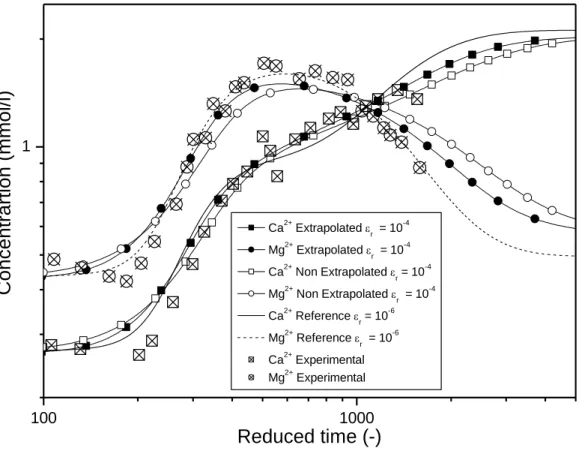
2 2  S Na Mg  S Mg  2 Na with K_NaMg 3.0 eq / L 15

In Figure 1, elution curves for calcium and magnesium given by the adaptive time step 16

with and without extrapolation are compared. A reference solution is obtained with a very 17

small precision criterion and is validated by comparison with experimental data given by 18

Valocchi et al. (1981). This figure illustrates clearly the increase of precision induced by the 19

extrapolation explained in equation (5). The extrapolated elution curve is closer to the 20

reference solution than the non extrapolated one. 21

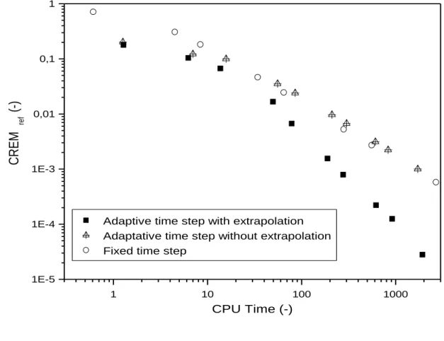
Using the extrapolated solution (5) or (22) leads to a more accurate solution at the cost of 22

computation, the extrapolation with adaptive time stepping presented in this work is very 1

efficient, as can be seen in Figure 2. CREMref has been calculated for each component and the

2

maximum value has been plotted. This figure shows that, as expected from the theory, a fixed 3

time step and an adaptive time step without extrapolation leads to a first order relation 4

between precision and CPU time. On the other hand, the combination of extrapolation and an 5

adaptive time step gives a second order relation between precision and CPU time. 6

7

3.2. UNSATURATED FLOW

8

The Richardson extrapolation has been studied for groundwater flow applications. Guarracino 9

et al. (2004) used the pressure head form of Richards’ equation and associated the

10

extrapolation with a Crank-Nicolson scheme to reach a third order accurate temporal scheme. 11

The authors did not insert a time-marching scheme and verified principally the accuracy and 12

the mass conservation properties. Besides, Basombrio et al. (2006) developed a competitive 13

non-iterative algorithm combining Crank-Nicolson method, Richardson extrapolation and a 14

single Newton’s iteration. However, the amplification or reduction factor for the time step is 15

quite heuristic. 16

17

3.2.1. Presentation of the model

18

The last example deals with the infiltration of water through an initially dry porous media. 19

The mathematical model used to describe this physical problem is given by equations (24) 20

and (25). 21

Darcy-Buckingham’s law defines the water flux in the domain: 22

  



q K h . hz , (24)

where q is the macroscopic fluid flux density, K is the hydraulic conductivity, h is the 1

pressure head and z is the depth, taken to be positive downwards. 2

The mixed form of Richards’ equation represents the mass conservation of water: 3

 

v h .q f t      , (25) 4

where θ is the volumetric water content, t is time, fv is a source/sink term, and q is the water

5

flux previously defined. 6

To complete this description, the interdependencies of the pressure head, the hydraulic 7

conductivity and the water content must be characterized using constitutive relations. The 8

standard Mualem - van Genuchten model (1980) is used : 9

 

 



 



 

 



  



   1 1/ n n r e s r 2 1 1/ n n / n 1 1/ 2 e s e e 1 h 0 h S h 1 h 1 h 0 K S K S 1 1 S     _     _  _      _      _   _   , (26) 10

where s and r are the saturated and residual volumetric water contents, respectively,  is a

11

parameter related to the mean pore size and n a parameter reflecting the uniformity of the 12

pore-size distribution (n>1). 13

The numerical technique implemented is a traditional finite volume method for the spatial 14

discretization and a backward Euler scheme for the temporal approximation. The interblock 15

conductivities, which appear for the calculation of the flux between adjacent cells of the 16

mesh, are calculated either with a geometric or an arithmetic mean. Due to the nonlinearities 17

of the constitutive relationships, we have to solve nonlinear partial differential equations. The 18

discretized system of PDE is linearized using the modified Picard (or fixed-point) method 19

(Lehmann and Ackerer, 1998). Iterations proceed until the mixed absolute-relative 20

n 1,k 1 n 1,k n 1,k

r a

i i i

h   h    h    , i =1,…,NN, (27)

1

where k denotes the iteration number. τa and τr refer to absolute and relative convergence

2

criteria. They are hundred times smaller than the corresponding criteria on the truncation error 3

tolerance. 4

5

3.2.2. Implementation of the time stepping method with the Richarsdon extrapolation

6

After each time step, the pressure head and the water content are updated with the Richardson 7 extrapolation: 8 n 1 n 1, n 1, n 1 n 1, n 1, h 2h h 2                  (28) 9

The temporal accuracy of the scheme has been considered as an important criterion. 10

However, the ability of the code to conserve good global mass balance is also essential. The 11

extrapolated solutions presented in (28) have no real physical meaning. To avoid a large mass 12

balance error, we suggested in a previous section to again solve the system with the 13

extrapolated solution at each time step with a higher order numerical scheme. Another 14

technique consists of extrapolating the flux. 15

16

3.2.3. Test case and discussion

17

We simulate a sharp infiltration front in a homogeneous dry porous media as proposed by 18

Celia et al. (1990). The initial, boundary conditions and the relevant material properties are 19

summarized in Table II. 20

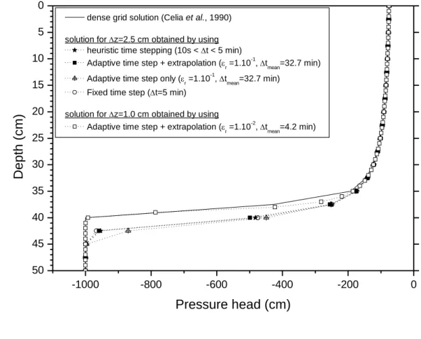
Figure 3 displays pressure head profiles after a half day of infiltration. The dense grid 21

solution provided by Celia et al. (1990) has also been plotted to show the convergence of the 22

arithmetic mean. Figure 3 illustrates the interest of the extrapolation compared to fixed time 1

step, time stepping scheme without extrapolation, or a heuristic time marching scheme based 2

on the behaviour of the nonlinear iteration. 3

To investigate temporal aspects of the Richardson extrapolation in unsaturated water 4

movement, a surrogate “reference” solution is evaluated numerically using the adaptive 5

scheme with a relative error tolerance of r = 10-8 and a convergence criterion of r = 10-10. An

6

identical fixed-grid with a nodal spacing of 1cm and a geometric interblock conductivity are 7

used for all simulations thus making it possible to neglect spatial errors and to focus only on 8

the temporal errors. 9

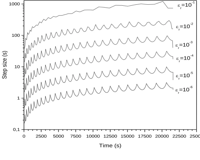
The proposed adaptive time stepping method allows the control of the temporal error with 10

the relative tolerance criterion r. An improvement of the precision coincides with the

11

automatic decrease of the step size by the algorithm as depicted in Figure 4. It shows a very 12

classical evolution of the step size. 13

We observe that reducing the relative precision criterion by a factor of one hundred leads to a 14

decrease of ten times the mean step size. In fact, the mean length of the time step reaches 450 15

seconds for the worst precision considered and just above 1 second for the largest. 16

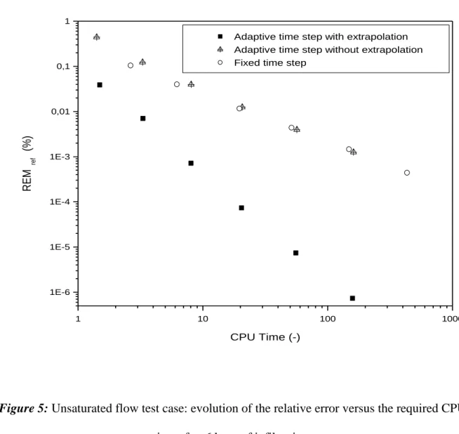
To analyse the efficiency of the method, the relative error has been plotted as a function of the 17

CPU time. Figure 5 is hence obtained by adjusting the criterion r for the adaptive scheme or

18

varying the time step size for the fixed step method. As shown in the previous example, 19

Figure 5 clearly illustrates that the algorithm using the Richardson extrapolation leads faster 20

to a higher accuracy. Hence, the adaptive time stepping method becomes competitive when 21

associated to the extrapolation. 22

It is all the more interesting because the mass balance can be correctly managed when 23

some precautions are taken into account. With a constant nodal spacing, the formula 24

 

















print init Ne n 1 0 n 1 0 n 1 0 1 1 i i Nn Nn i 2 time j j j 1 Nn j time 1 1 x 2 2 GMB % 1 100 q q t                                





(29) 1

The fluxes that appear in the previous equation can be estimated using a variety of means. If 2

the extrapolation is used at each time step for the error estimation and the variable adaptation, 3

the flux can be calculated through a first (totally implicit formulation) or a second (Crank-4

Nicolson formulation) order approximation. Nevertheless, Figure 6 shows that the best 5

technique is to also extrapolate the flux. If the variables obtained in two time steps are 6

retained, Figure 6 also illustrates that the flux can not be viewed as a general flux on this 7

period calculated with the last pressure. This must be calculated after each half time step. 8

9

4. Conclusion

10

After a brief presentation of the Richardson extrapolation, this paper has described a general 11

way of taking into account the truncation error for an efficient management of the step size 12

evolution. The automatic time marching scheme is mathematically based and the user must 13

only define the accepted tolerance on the temporal discretization error. Another important 14

aspect of this work deals with optimisation strategies to estimate the first time step, to 15

implement the algorithm in a nonlinear system, or to introduce flexibility in the time 16

evolution, i.e., to avoid too many rejected time steps. The whole of our approach was 17

developed in a context that could allow its application to diverse numerical fields. This 18

algorithm can easily take into account specificities of a given problem. 19

In fact, all our propositions have been implemented in rather different codes that model 20

algorithm allows treatment of notably different mathematical models. The proposed method is 1

an efficient way of adapting the time step size and of estimating the error for many problems 2

frequently encountered in porous media. 3

The use of extrapolation technique appears advantageous. First, the examples show that the 4

accuracy has been improved. For a given error calculated with a reference solution, the 5

extrapolation of the variables yields a decrease in computation time compared to both a fixed 6

time step or an adaptive evolution without extrapolation. Second, although extrapolation may 7

not always have physical meaning, it can still conserve properties as illustrated in our 8

example mass balance calculation. 9

Future research could deal with a comparison of different time marching schemes, a spatial 10

adaptation coupled with the time stepping strategy, or a separate time stepping procedure for 11

the transport and reaction operators involved in the splitting method. 12

13 14

Acknowledgments

15

The authors sincerely thank the seven anonymous reviewers and Paul Montgomery (CR-HDR 16

CNRS Strasbourg) for their suggestions for improvements. 17

References:

1

Abbasian, R. O. and Carey, G. F.: 1997, A note on Richardson extrapolation as an error 2

estimator for non-linear reaction-diffusion problems, Commun. Numer. Meth. Engng., 13 3

(7), 533-540. 4

Aïd, R.: 1999, Richardson estimator with variable step-size, C. R. Acad. Sci. Paris, 329 (I), 5

833-837. 6

Ayati, B. P. and Dupont, T. F.: 2004, Convergence of a step-doubling galerkin method for 7

parabolic problems, Math. Comput., 74 (251), 1053-1065. 8

Babuska, I. and Rheinboldt, W. C.: 1978, A posteriori error estimates for finite element 9

method, Int. J. Numer. Methods Engng., 12 (10), 1597-1615. 10

Bank, R. E. and Smith, R. K.: 1993, A posteriori error estimates based on hierarchical bases, 11

SIAM J. Numer. Anal., 30, 921–932.

12

Basombrio, F. G., Guarracino, L. and Vénere, M. J.: 2006, A non-iterative algorithm based on 13

Richardson’ extrapolation. Application to groundwater flow modelling. Int. J. Numer. 14

Meth. Engng., 65 (7), 1088-1112.

15

Bause, M. and Merz, W.: 2005, Higher order regularity and approximation of solutions to the 16

Monod biodegradation model, Appl. Numer. Math., 55 (2), 154-172. 17

Carrayrou, J., Mosé, R. and Behra, Ph.: 2002, New efficient algorithm for solving 18

thermodynamic chemistry, AIChE. J., 48 (4), 894-904. 19

Carrayrou, J., Mosé, R. and Behra, Ph.: 2003, Modelling reactive transport in porous media: 20

iterative scheme and combination of discontinuous and mixed-hybrid finite elements, C. R. 21

Mec., 331 (3), 211-216.

22

Carrayrou, J., Mosé, R. and Behra, Ph.: 2004, Efficiency of operator splitting procedures for 23

Celia, M. A., Bouloutras, E. T. and Zarba, R. L.: 1990, A general mass-conservative 1

numerical solution for the unsaturated flow equation, Water Resour. Res., 26 (7), 1483-2

1496. 3

Claramunt, K., Cònsul, R., Pérez-Segarra, C.D. and Oliva, A. : 2004, Multidimensional 4

mathematical modeling and numerical investigation of co-flow partially premixed 5

methane/air laminar flames, Combust. Flame, 137 (4), 444-457. 6

Guarracino, L. and Quintana, F.: 2004, A third-order accurate time scheme for variably 7

saturated. Commun. Numer. Meth. Engng., 20 (5), 379-389. 8

Hairer, E., Nörsett, S. P. and Wanner, G.: 2000, Solving Ordinary Equations I, Nonstiff 9

problems, 2nd edition, Springer-Verlag, Berlin, pp 528.

10

Kavetsky, D., Binning, P. and Sloan, S. W.: 2001, Adaptative time stepping and error control 11

in a mass conservative numerical solution of the mixed form of Richards equation, Adv. 12

Water Resources, 24 (6), 595-605.

13

Lehmann, F. and Ackerer, P.: 1998, Comparison of iterative methods for improved solutions 14

of the fluid flow equation in partially saturated porous media, Transp. Porous Media, 31 15

(3), 275-292. 16

Liao, W., Zhu, J. and Khaliq, A. Q. M. : 2002, An efficient high-order algorithm for solving 17

systems of reaction-diffusion equations, Numer. Meth. Part. Differ. Equ., 18 (3), 340-354. 18

Natividad, M.C. and Stynes, M.: 2003, Richardson extrapolation for a convection-diffusion 19

problem using a Shishkin mesh, Appl. Numer. Math., 45 (2-3), 315-329. 20

Richards, S. A.: 1997, Completed Richardson extrapolation in space and time, Commun. 21

Numer. Meth. Engng., 13 (7), 573-582.

22

Richardson, L. F.: 1910, The approximate arithmetical solution by finite difference of 23

physical problems involving differential equations, with an application to the stress in a 24

Richardson, L. F.: 1927, The deferred approach to the limit. I: single lattice, Philos. Trans. 1

Roy. Soc. London, 226 (A), 299-349.

2

Rubin J.: 1983, Transport of reacting solutes in porous media : relation between mathematical 3

nature of problem formulation and chemical nature of reaction, Water Resour. Res., 19 (5), 4

1231-1252. 5

Schneid, E., Knabner, P. and Radu, F.: 2004, A priori error estimates for a mixed finite 6

element discretization of the Richards’ equation, Numer. Math., 98 (2), 353-370. 7

Shampine, L. F.: 1985, Local error estimation by doubling, Computing, 34 (2), 179-190. 8

Steefel, C. I. and McQuarrie, K. T. B.: 1996, Approaches to modelling of reactive transport in 9

porous media. In Reactive Transport in Porous Media. P. C. Lichtner, C. I. Steefel, E. H. 10

Oelkers, Eds., Reviews in Mineralogy, Mineralogical Society of America, Washington. 34,

11

82-129. 12

Sun, S. and Wheeler, M. F.: 2005, Discontinuous Galerkin methods for coupled flow and 13

reactive transport problems, Appl. Numer. Math., 52 (2-3), 273-298. 14

Valocchi, A. J., Street, R. L. and Roberts, P. V.: 1981, Transport of ion-exchanging solutes in 15

groundwater: Chromatographic theory and field simulation, Water Resour. Res., 17 (5), 16

1517-1527. 17

van Genuchten, M. Th.: 1980, A closed-form equation for predicting the hydraulic 18

conductivity of unsaturated soils, Soil Sci. Soc. Am. J., 44 (5), 892–898. 19

Yeh, G. T. and Tripathi, V. S.: 1989, A critical evaluation of recent developments in 20

hydrogeochemical transport models of reactive multichemical components, Water Resour. 21

Res., 25 (1), 93-108.

22

Zienkiewicz, O. C. and Zhu, J. Z.: 1992, Superconvergent patch recovery and a posteriori 23

error estimates. Part 2: error estimates and adaptivity, Int. J. Numer. Methods Engng., 33 24

Index

1 Abstract ... 2 2 1. Introduction ... 2 3

2. Presentation of the method ... 5 4

2.1. extrapolation ... 5

5

2.2. time step size adaptation ... 6

6

2.3. optimisation of the method ... 8

7

2.3.1. Relative test and tolerance on the precision criterion ... 8 8

2.3.2. Selection of the first time step ... 9 9

2.3.3. Implementation for nonlinear ODE or PDE ... 10 10

3. Examples ... 11 11

3.1. reactive transport with operator splitting ... 12

12

3.1.1. Presentation of the model ... 13 13

3.1.2. Implementation of the time stepping method with the Richardson extrapolation . 14 14

3.1.3. Test case and discussion ... 15 15

3.2. unsaturated flow ... 16

16

3.2.1. Presentation of the model ... 16 17

3.2.2. Implementation of the time stepping method with the Richarsdon extrapolation . 18 18

3.2.3. Test case and discussion ... 18 19 4. Conclusion ... 20 20 Acknowledgments ... 21 21 References: ... 22 22 Index ... 25 23 List of Tables ... 26 24 Figure Captions ... 26 25 26 27

List of Tables

1

Table I: Physico-chemical parameters for the reactive transport test-case. ... 27 2

Table II: Initial, boundary conditions and parameters values for the unsaturated flow 3 test case. ... 28 4 5

Figure Captions

6

Figure 1: Reactive transport test case: comparison of the elution curves. ... 29 7

Figure 2: Reactive transport test case: evolution of the Cumulated Relative Error 8

Measure (CREMref) versus the required CPU time. ... 30

9

Figure 3: Unsaturated flow test case: Pressure head profiles after 12 hours of 10

infiltration. ... 31 11

Figure 4: Unsaturated flow test case: evolution of the time step size versus time for the 12

scheme with extrapolation. ... 32 13

Figure 5: Unsaturated flow test case: evolution of the relative error versus the required 14

CPU time after 6 hour of infiltration. ... 33 15

Figure 6: Unsaturated flow test case: representation of the mass balance function of 16

the relative precision criteria: comparisons of different techniques for the 17

flux approximation. ... 34 18

19 20

1

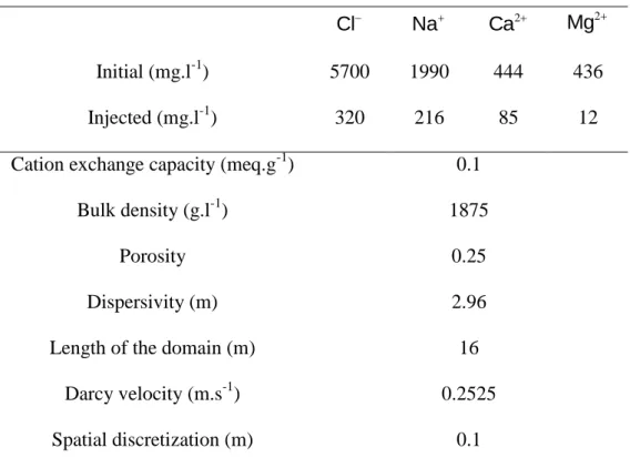
Table I: Physico-chemical parameters for the reactive transport test-case. 2 3 Cl Na 2 Ca Mg2 Initial (mg.l-1) 5700 1990 444 436 Injected (mg.l-1) 320 216 85 12

Cation exchange capacity (meq.g-1) 0.1

Bulk density (g.l-1) 1875

Porosity 0.25

Dispersivity (m) 2.96

Length of the domain (m) 16

Darcy velocity (m.s-1) 0.2525 Spatial discretization (m) 0.1 4 5 6 7 8

1

Table II: Initial, boundary conditions and parameters values for the unsaturated flow test 2 case. 3 4 Parameters Value Material and/or Reference sand Celia et al. (1990) r (-) _0.102 s (-) _0.368  (cm-1) 0.0335 n (-) 2 Ks (cm.s-1) 9.22 10 3 Initial conditions h(z,t=0) (cm) -1000 Boundary conditions h(z=0 cm,t) (cm) -75 h(z=100 cm,t) (cm) -1000 5 6 7 8 9

1 100 1000 1 C o n ce n tra rt io n (mmo l/ l) Reduced time (-) Ca2+ Extrapolated _r = 10-4 Mg2+ Extrapolated _r = 10-4 Ca2+ Non Extrapolated _r = 10-4 Mg2+ Non Extrapolated _r = 10-4 Ca2+ Reference _r = 10-6 Mg2+ Reference _r = 10-6 Ca2+ Experimental Mg2+ Experimental 2 3

Figure 1: Reactive transport test case: comparison of the elution curves. 4 5 6 7 8 9

1 1 10 100 1000 1E-5 1E-4 1E-3 0,01 0,1 1 C R EM re f (-) CPU Time (-)

Adaptive time step with extrapolation Adaptative time step without extrapolation Fixed time step

2 3

Figure 2: Reactive transport test case: evolution of the Cumulated Relative Error Measure 4

(CREMref) versus the required CPU time.

5 6 7 8 9 10

50 45 40 35 30 25 20 15 10 5 0 -1000 -800 -600 -400 -200 0 Pressure head (cm) D e p th (cm)

dense grid solution (Celia et al., 1990)

solution for z=2.5 cm obtained by using heuristic time stepping (10s < t < 5 min) Adaptive time step + extrapolation (

r =1.10 -1

, t

mean=32.7 min)

Adaptive time step only (_r =1.10-1, t_mean=32.7 min) Fixed time step (t=5 min)

solution for z=1.0 cm obtained by using

Adaptive time step + extrapolation (_r =1.10-2, t_mean=4.2 min)

1 2

Figure 3: Unsaturated flow test case: Pressure head profiles after 12 hours of infiltration. 3

1 0 2500 5000 7500 10000 12500 15000 17500 20000 22500 25000 0,1 1 10 100 1000  r=10 -6  r=10 -5  r=10 -4  r=10 -3  r=10 -2 St e p si ze (s) Time (s)  r=10 -1 2 3

Figure 4: Unsaturated flow test case: evolution of the time step size versus time for the 4

scheme with extrapolation. 5 6 7 8 9 10

1 1 10 100 1000 1E-6 1E-5 1E-4 1E-3 0,01 0,1 1 R EM re f (% ) CPU Time (-)

Adaptive time step with extrapolation Adaptive time step without extrapolation Fixed time step

2 3

Figure 5: Unsaturated flow test case: evolution of the relative error versus the required CPU 4

time after 6 hour of infiltration. 5

6 7

1

1E-6 1E-5 1E-4 1E-3 0,01 0,1

1E-9 1E-8 1E-7 1E-6 1E-5 1E-4 1E-3 0,01 0,1 1 Ma ss b a la n ce (% ) Precision criteria  r(-)

without Richardson extrapolation: flux calculated after each half time step flux calculated after the second half time step

with Richardson extrapolation: extrapolated flux

flux calculated with extrapolated solution (2nd order) flux calculated with extrapolated solution (1rst order)

2 3

Figure 6: Unsaturated flow test case: representation of the mass balance function of the 4

relative precision criteria: comparisons of different techniques for the flux approximation. 5 6 7 8 9 10 11