Cooling of underground transmission lines : heat transfer measurements

(1)

PART I OF IV

COOLING OF UNDERGROUND TRANSMISSION LINES: FEAT TRANSFER MEASUREMENTS

by Robert A. Slutz William P. Orchard Leon R. Glicksman Warren M. Rohsenow Energy Laboratory in association with Heat Transfer Laboratory, Department of Mechanical Engineering

MASSACHUSETTS INSTITUTE OF TECHNOLOGY

(

A

(2)

The heat dissipated in the conductor of a forced cooled pipe type cable must pass through two thermal resistances in series: the conduction resistance of the cable insulation and the convection resistance due to forced and natural convection from the cable surface to the oil. The upper limit to the convection resistance was determined by natural convection heat transfer tests on a full scale model of a pipe type cable system. It was

found that conduction resistance is more than four times larger than convection resistance for cables designed for 138 kv and higher voltages. Therefore, to accurately predict the temperature inside the cable for a given oil temperature and current, a precise prediction of convection heat transfer is necessary. The solution for conduction within the cable must include effects due to cablesplices and the proximity of one cable to another.

(3)

This study was sponsored by the Consolidated Edison Company of New York. We would like to thank Mr. Michael Buckweitz, Dr. Howard Feibus, and Mr. Frank Fischer of Consolidated Edison for their assistance.

(4)

List of Symbols

A - Area (ft

)

C = heat capacity (BTU)

R = heat flow resistance (F hr ft/BTU)

T = temperature (F)

t = pipe wall thickness (ft)

U = local heat transfer coefficient between a point on the cable surface and the cooling wall (BTU/hr ft2°F)

Ui = overall heat transfer coefficient between cable i and the wall, using the

1 ~~~~~~~~~~~~~~~2

average temperature of the cable (BTU/hr ft °F)

U = average heat transfer coefficient between all 3 cables and the wall using

S~~~~~~~~~~~~~~~~

the wetted area of the wall (BTU/hr ft2 F)

h - local heat transfer coefficient between a point on the cable surface and the oil (BTU/hr ft2 F)

K = thermal conductivity (BTU/hr ft°F)

q = heat flux (BTU/hr)

(5)

INTRODUCTION

A high-pressure, oil-filled, pipe-type cable system used for underground electrical power transmission is made up of several cables enclosed in a steel pipe. The cables are constructed with a copper conductor wrapped with porous, oil-soaked paper insulation and a protective outer covering. The space between the cables and the pipe is filled with a dielectric oil which is under high pressure. The oil, which impregnates the paper wrapping on the cables, provides electrical insulation for the cables and, at the same time, transfers the heat generated by losses in the cables to the pipe and surrounding earth. Pressur-ization of the oil prevents vapor formation in the paper insulation and insures proper electrical insulation of the cables. The power carrying capacity of underground cables is limited by the maximum allowable conductor temperature, which in turn depends on the rate of heat removal from the system.

Forced cooled systems for oil-filled pipe-cable circuits have recently been considered. Chilled oil is circulated through the pipe, and most of the heat generated in the cable and insulation is absorbed by the oil. The heat is transferred from the oil to the atmosphere at refrigeration stations. By use of a forced cooled system the power capacity of underground cable systems can be economically increased.

In a forced cooled system the heat dissipated within the conductor is transferred by conduction through the cable insulation to the surface of the cable. The heat is transferred to the oil by a combination of forced and natural convection. The forced convection is established by the throughflow of the oil and the natural convection set up by the temperature difference between the cable and the oil. Thus, the heat dissipated in the conductor must pass through two thermal resistances in series: the conduction resistance in the paper insulation and the combined forced and natural convection resistance at the outer surface of

the cable.

There are no previous heat transfer studies available for the configuration in question. Neher and McGrath [1] present an approximate relationship based on correlations for a much simpler geometry. The accuracy of their analytical development remains open to question.

The present investigation was undertaken to determine the relative magnitude of the conductive to the convective resistances. Although there has not been any reliable measurements of convective heat transfer for the cable pipe geometry in question, results for simple geometries tend to indicate that the convective heat transfer resistance should be negligible in comparison to the conductive

(6)

resistance through the insulation. If this can be verified. the solution of the temperature distribution in the cable with forced cooling can be simplified to a study of the conduction effects in the insulation.

The value of the conduction resistance can be calculated analytically but the convective resistance must be experimentally measured. Measurement of combined forced and natural convection is difficult to accomplish because the region of entrance effects for forced convection heat transfer in oils is very long; e.g. for oil flow with a Reynolds number of 1000 and a Prandtl number of 50 fully developed flow does not occur until the length to diameter ratio exceeds 5,000. In the entrance region the heat transfer may be as much as an order of magnitude higher than the heat transfer for fully developed flow [2] thus entrance

region results will give erroneously low values of thermal resistance. The

requirement for a large L/D suggests the use of a scaled down model. However, to correctly scale both the effects of forced and natural convection, the following dimensionless quantites must be the same as the full sized system: Reynolds number, Prandtl number and Grashof number. No fluid could be found which would satisfy this requirement in a scaled down model.

To circumvent the modelling and the entrance length problems, a natural

convection test on the full sized system was made. Since forced convection should augment natural convection heat transfer, the thermal resistance for natural

convection alone should be higher than the thermal resistance for combined natural and forced convection. If the thermal resistance for natural convection is much smaller than the conduction resistance through the cable insulation, then it is reasonable to assume that the thermal resistance for combined natural and forced convection should be smaller than the conduction resistance.

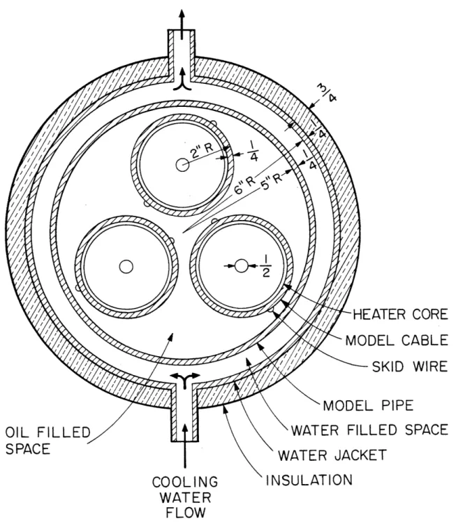
Figures 1 and 2 show the dimensions of the cable system which was studied.

The outer steel pipe has an inside diameter of 10.25 inches and encloses three cables each about four inches in diameter. The cables each have a central copper conductor which is wrapped first with paper insulation, then with a protective mylar covering

and, lastly, with skid wires. The skid wires protect the cable coverings and reduce friction when the cables are being pulled into the pipe.

EXPERIMENTAL PROGRAM

Experimental data were taken on a full sized model of an underground cable system. Figure 3 is a cross section of the model. The model cables shown in Figures 4, were made from 4" OD steel pipe inside of which were heaters to produce

(7)

the desired heat flux. Each cable, which was 4 feet in length, was made in 3 equal sections thermally insulated from each other to allow for end effects. The middle section was used for test data.

The heaters were made with glass cores around which heater wire was wound. The assembly was then coated with a thermally conductive epoxy poste and inserted

into sections of the 4" pipe. Insulating spacers were placed between sections and three sections were held together by means of central threaded rod and threaded end plates. Each section had a separately controlled heater.

Semi-circular steel skid wires were wound around the outside of the 4" cables and held in place with tack welds.

The pipe part of the model was made of a 4 foot long section of 10 inch I.D. steel pipe. A section of 12 inch pipe was fitted around the 10 inch pipe to create a water jacket. Cooling water was circulated through the annulus at a high flow rate to provide good heat transfer between the pipe wall and the water. This produced a constant wall temperature around the circumference of the pipe.

The ends of the pipe were closed by means of cover plates, one of which allowed the heater and thermocouple wires to pass through. The space between the 10 inch pipe and the 3 "cables" was filled with a dielectric oil. Two

oils were used to give values at very high and very low viscosity: high viscosity polybutane and pure tridcylbenzene. A total of fourteen thermocouples were

fastened to each test section at six locations around the circumference and at 4 axial locations. Three thermocouples were fastened to the inside of the pipe wall at the bottom, side, and top. Three thermocouples were mounted on adjustable probes with micrometers to allow measurement of the oil temperature profile. A potentiometer was used to read the thermocouple outputs. The power level in the heaters was measured with a precision watt-meter. Each heater was individually

controlled with a variable transformer so that the end sections were at the same temperature as the central test section.

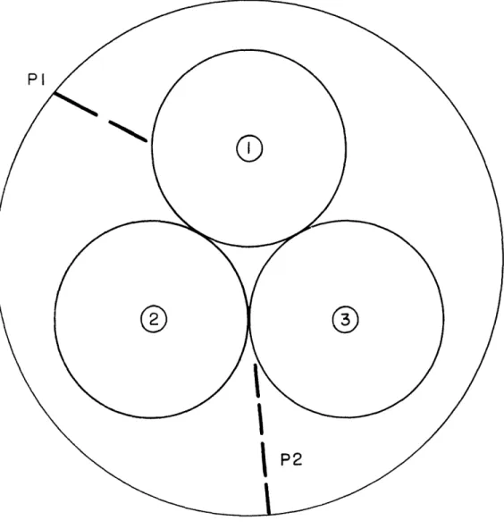
Three configurations were chosen for study and these are shown in Figure 5. The general characteristics of each are:

Configuration I - 3 cables touching each other but not touching the wall. II - no points of contact between the cables or wall.

III - cables touching each other and the cooling wall.

Detailed temperature profiles were made for each configuration to determine the existence and location of regions of constant temperature in the oil.

(8)

ANALYSIS

The desired result of the heat transfer work is a comparison between the resistance to natural convection from the surface of the cable to the oil and the resistance to conduction through the cable insulation. The equation defining the resistance to heat transfer per unit length is:

AT

L R (1)

where q is the total heat flow. AT is the temperature difference driving the heat flow, L is the axial length and R is the resistance to heat flow.

The heat flow due to conduction in the cable insulation assuming purely radial heat flow is (from 2])

q 2i k AT

(2)

L

)~~~~~~~~~~~~~~2

L- n(r2/r₁₎

where k is the conductivity of the insulation and r₁ and r₂ are the inner and outer radii of the insulation. Solving (1) and (2) for R gives:

£n (r2/r )

R = 2 k (3)

for the resistance per unit length.

The natural convection data will be given in terms of 4 heat transfer coefficients which are defined as follows:

1) h = () /(T -T ) (4)

A cable cable oil

- a local heat ransfer coefficient between a point on the cable surface and the ambient oil.

2) U = () /(Tcabl_e T wa(5) A cable cable wall

- a local heat transfer coefficient between a point on the cable surface and the pipe wall.

3) U = () /(Ti wall) (i = 1,2, or 3) (6)

cable

- the overall heat transfer coefficient between each cable and the wall, using T, the average temperature of the cable, and the wetted area of one cable.

(9)

4 )U =(3 /(T- -T

)7

wall wall

- the average heat transfer coefficient between all 3 cables and the wall, using the wetted area of the wall.

Knowing the dimensions of the apparatus, these coefficients can readily be converted to thermal resistances by the relationship:

R -h(A/L) (8)

The local heat transfer coefficients were calculated from the measured heater power inputs and the measured temperatures of the cable, oil and wall. In performing the calculations it was assumed that the heat transferred per unit area from the cable to the oil is constant over the entire surface area of the cable. A uniform heat flux from the cable requires a uniform heat flux from the heaters to the cable surface and negligible circumferential and axial conduction through the steel pipe representing the cable surface. RESULTS

For each configuration a detailed temperature profile of the oil was made with the thermocouple probes. Typical results are shown in Figures 6 - 8. This procedure allowed the identification of large constant temperature regions in the oil. These temperatures were then used to calculate the local heat transfer coefficients from the surface of the cable to the oil.

Note the distinct thermal boundary layer regions in Figures 6-8 near the cable and the pipe wall. These are not present in some of the regions at the bottom of the tube because the hot cables are above the cold pipe wall, a condition which minimizes convective motion. For the latter regions, h was based on an artificial ambient temperature: simply the mean of the cable and the pipe wall temperature. Heat transfer coefficients so defined are starred throughout the data presentation.

The convection heat transfer coefficient, h, is of central importance since it can be used to compare the convection resistance between the cable surface and the main body of oil with the conductive resistance through the paper insulation.

(10)

The results of the experiments are summarized in Tables 1, 2, and 3. In the table, the power input represents the power to the central test section of each cable. The oil temperature is that of the isothermal region between

the pipe and the cable, e.g. see Fig. 6B. U3 is higher than U1, U2, and U3

since the former is based on the wetted area of the pipe wall and the latter

is based on the wetted area of a cable.

An estimation of the maximum circumferential conduction around the 4 inch pipes can be made using the data for configuration 3, where the temperature varies

9°F in a 90° arc. The ratio of the heat conducted around the 90° arc to the heat

transferred to the oil in the same arc is at most one tenth.

Figure 9 shows the Nusselt number,a nondimensionalized h, as a function of the Rayleigh number for the upper cables in each configuration. Nu and Ra are based on cable diameter.

As expected, h increases as the fluid viscosity decreases and as the temp-erature difference causing bouyancy effects increases. Figure 9 also shows the theoretical results for natural convection from a single horizontal tube in an infinite medium (without any confining walls). The present results tend to follow the same general trend as the theory at these high Rayleigh numbers because a rather thin thermal boundary layer forms on the cable and pipe walls,

and the interaction between the cable and the pipe wall is minimized. This is analogous to the natural convection between two parallel vertical plates one cold and the other hot. At high Rayleigh numbers, the natural convection boundary layer on the plate approaches that found on a single plate in an

infinite medium. It must be emphasized that good quantitative agreement between the simple geometry and the case at hand is not achieved nor should it be

expected. Eckert and Soehngen [3] have shown that when a horizontal cylinder is placed directly above another cylinder, the Nusselt number of the top cylinder is lower than the single cylinder value. However, when the cylinders are stag-gered the Nusselt number of the top cylinder is increased.

Figure 10 shows the average heat transfer coefficient from the three cables to the pipe wall. In this figure, Nu and Ra are based on the hydraulic diameter, equal to 2.66 inches, and all oil properties are evaluated at the mean of the

cable and pipe wall temperature. Note that the average coefficients change in-significantly from one cable configuration to another. Also shown in Figure 10 is the initial correlation used b1y Buller and Neher [4]. This correlation over-predicts the heat transfer coefficient by one third and thus underover-predicts the

(11)

thermal resistance by an equal amount. This error does not result in a significant error in the overall heat transfer for either the forced cooled or the natural cooled case since the oil resistance is negligible for both cases.

COMPARISON OF HEAT TRANSFER RESISTANCES

The experiments described in this report were primarily performed to test

the hypothesis that conductive heat transfer resistance through the cable insulation is much higher than convective resistance from the cable to the oil. Assuming

the thermal conductivity of the oil soaked paper insulation is the same as that of the oil yield a conductive resistance of

R = 2.18 ft hr°F/BTU (9)

cond

Using the highest value of paper conductivity reported by Neher and McGrath [2] reduces this value by only 40 percent. Using the smallest values of h given in

table 4 for the viscous oil and further reducing it to correspond to a AT of 5°F ( assuming h is proportional to (AT)1 / 4) gives an h of 4.1 BTU/hr ft2° F. The corresponding resistance is

R = 1 = 1 = 0.23 ft hr°F/BTU (1)

convective hA/L

hrrD

Therefore the resistance is one order of magnitude lower than the conductive resistance. Since the heat flows from the central conductor of each cable through the conductive and convective resistances in series, the convective resistance has a negligible effect on the heat flow.

Table 4 gives the results for a range of geometries used in pipe type cable systems. For each geometry h was calculated from figure 9, which is valid since each geometry had approximately the same cable to pipe diameter ratio. The assumption of negligible convection resistance is open to question only for the 69 KV cables. Cables designed for voltages higher than 345 KV will have even

thicker insulation and thus will conform very closely to the assumption of negligible convective resistance.

MOST CONSERVATIVE ESTIMATE

In evaluating the convective resistance for forced cooled cables the absolutely worst case would involve the lower oil-filled region of configuration II with these

(12)

No oil throughflow in the lower oil-filled region and no mixing the oil in the other regions.*

No heat transfer to the soil, i.e. an adiabatic outside pipe surface.

In this case the heat leaving the cable surface in contact with the lower region must be transferred across the oil to the pipe. The heat must flow cir-cumferentially around the pipe, and must then be transferred to the cool flowing oil in the upper region, see Figure 11. The pipe surface of length S acts like a fin, receiving heat along its inside surface and transferring it circumferentially by conduction. Assuming a constant heat transfer coefficient, U, between the

surface of the cable and the pipe surface, the temperature difference between the cable and the pipe, at the base of the "fin" is

T - T = (qo/L) /U Kt tanh S/K t (11)

c p p p

where t is the pipe wall thickness, K is the thermal conductivity of the pipe,

P

and q is the total heat flux transferred to the pipe.

Similarly, the heat transferred from the pipe to the cool oil is a second fin problem with a constant heat transfer coefficient h between the pipe wall and the cooler oil. For this case we can assume the circumferential length of the pipe is long so that the hyperbolic tangent is unity. Therefore,

T - T = (o/L)/7 Kt (12)

p o p

Adding equation (11) and (12) the overall temperature difference is,

T - T = qo/L 1 + 1 ] (13)

c o

_~c

_o _{Ah K t} _{VU K t tanh S U/K t}

p P p P pP

q represents the amount of heat from the cylinder surface which is transferred to the non-flowing oil, i.e. the amount of heat transferred over the angle of the cylindrical surface as shown in Figure 11. Inside the cable insulation, assuming one-dimensional conduction,

q /L = (T

qI=

T

I₁ -

TcKo

Tc) K 0

(14)

0 ln (r2/rl)

2 1

*This is an extreme assumption made to yield the most conservative estimate. In actual fact, there will always be some oil flow through the lower section

and the liklihood of this cross-section persisting very far down the pipe is small, i.e., at intervals along the pipe the cables will be shifted, allowing oil

(13)

Combining equation 13 and 14 to eliminate q/L and rearranging, T -T K 0 c o0 o 0

v

1 1 1 T. )+ T 1] (15) I c ln(r2 r1 +U t V K tanh SU/K t P P P

Using the most conservative values for U and h of 1.6 and 3.3 BTU/hr ft°F respectively, based on the very viscous oil with a AT of 5F, the ratio of the temperature drop across the cable insulation to the temperature drop from the cable surface to the cooling oil is 2.5/1. Bearing in mind that this result is for the most conservative conditions, i.e. the conditions yielding

the largest cable to cooling oil temperature drop, it is safe to assume in all cases that the thermal resistance through the cable insulation is the controlling resistance for forced cooled cables.

CONCLUSIONS

For a pipe type cable system designed for 138 KV or higher voltages, the thermal conduction resistance across the cable insulation is an order of magnitude larger than the convection resistance from cable surface to

the oil. Therefore, to accurately predict the cable temperature the conduction within the insulation must be accurately modelled whereas a precise prediction of the convection outside the cable is not necessary. The solution for the

conduction within the insulation must include effects due to cable splices and the proximity of one cable to another. The most severe case is three cables in an equilateral triangular configuration with stagnant oil trapped between the three cables. When two cables and the pipe wall form a confined oil space,

temperature conditions are not as severe since the pipe forms a rather good conduction path between the confined oil and cooler oil outside of the confined space.

(14)

References

1. Neher, J.H. and McGrath, M.H., "The Calculation of the emperature Rise and Load Capability of Cable Systems," AIEE Trans, Part III, Vol. 76, pp. 752-772, October 1957.

2. Rohsenow, W.M. And Choi, H., Heat, Mass and Momentum Transfer, Prentice Hall, 1961, Englewood Cliffs, N.J.

3. Eckert, E.R.G. and Soehngen, E., Studies 6n heat transfer in laminar free convection with the Felider-Mach Interferometer. Tech. Report No. 5747, USAF, Air Material Command, Dayton, Ohio, 1948.

4. Buller, F.H. and Neher, J.H., "Thermal Resistance Between Cables and A Surrounding Pipe or Duct Wall," AIEE Trans, Vol. 69, pt4 I, 1950, pp. 342-349.

(15)

Heat Flux BTU/hr/ft2 122 183 311

Watts/heater (3 per cable) 50W 75W 128W

1) Oil Temperature, T (°F) 86.3 91.0 102.7

Pipe Wall Temperature (F) Bottom 70.9 71.3 71.3

Top 73.0 74.1 76.5

2) h (with corresponding cable Local Heat Transfer Coefficient

temperature) Cable Surface to Oil

h (BTU/hr ft2oF) ~~CABLE 1 L (/11.3 (97.1) 12.4 (105.7) 16.3 (121.7) hR 11.1 (97.3) 12.2 (106.0) 15.9 (122.4) hT hCABLE 2 T 17.4 (93.3) 18.1 (101.0) 24.4 (115.4) CABLE 2 hB 12.3*(90.9) 14.0* (97.9) 19.5* (108.0) CABLE 3 h15.6 (94.1) 15.4 (102.9) 20.8 (118.0) hB

~~~~~~3)

~Local

U Heat Transfer Coefficient

3) U Cable Surface to Pipe Wall

U (BTU/hr ft2°F) CABLE 1 UR 4.9 5.6 6.6 UCABLE 2 T 5.9 6.6 7.8 CABLE 2 B 6.1 6.9 8.5 UT 5.7 6.2 7.3 CABLE 3 UB

- Average Heat Transfer Coefficient

4) U₁,₂,₃ for each Cable to Wall

U1 4.8 5.1 6.4

U2 5.9 6.7 6.4

U3 5.8 6.6 7.7

5) U Overall Heat Transfer Coefficient

Three Cables to Wall

(16)

Configuration II

Heat Flux BTU/hr/ft2 Watts/heater

1) Oil Temperature (F) T T o

Pipe Wall Temperature, Bottom Top 2) h (with corresponding cable

temperature) h_L(BTU/hr ft °F) CABLE 1 hR hC hT CABLE 2 hB hc hT CABLE 3 hB h C 3) U UL (BTU/hr ft2 °F) CABLE 1 UR UT CABLE 2 UB UT CABLE 3 UB 4) U1,2,3 U1 U3 5) U_S 122 183 305 50 75 125 87.0 86.4 91.7 101.4 71.0 70.6 70.7 73.7 74.4__ 7,74 __

Local Heat Transfer Coefficient Cable Surface to Oil

11.8 (96.7) 14.1 (104.7) 16.5 (119.7) 10.9 (97.5) 13.3 (105.5) 15.9 (120.8) 11.6 (97.5) 18.2 (93.2) 20.6 (100.6) 24.8 (113.5) 12.3*(90.8) 13.8* (97.2) 16.1*(108.5) 15.4 (94.2) 17.4 (102.2) 20.8 (116.2) 16.7 (94.3)

Local Heat Transfer Coefficient Cable Surface to Pipe Wall

5.2 5.9 6.0

5.0 5.6 6.8

6.1 6.5 7.7

6.2 6.9 8.1

5.8 6.2 7.2

Average Heat Transfer Coefficient for each Cable to Wall

5.1 5.8 6.8

5.9 6.5 7.7

5.8 6.5 7.6

Overall Heat Transfer Coefficient 6.76

I

7.59

1

3.92 Table II

i

(17)

Configuration III Table III

Heat Flux BTU/hr/ft 122 183 305

Watts/heater 50 75 125

1) Oil Temperature, T (°F) 87.5 91.9 102.0

O

Pipe Wall Temperature, Bottom 71.2 70.9 71.0

Top 71.6 72 .1- 75.0

2) h (with corresponding cable Local Heat Transfer Coefficient

temperatures) Cable Surface to Oil

hT(BTU/hr ft 2.F) 19.4 (93.8) 21.5 (101.5) 23.5 (116.5) CABLE 1 hL 11.2*(89.3) 13.1*(95.5) 14.6*(107.4) hR 10.7*(89.8) 13.1*(95.5) 14.5*(107.6) hT 15.8 (95.2) 15.8 (103.5) 19.1 (118.0) CABLE 2 hR 14.9 (95.7) 15.8 (103.5) 18.9 (118.1) hB 8.4*(93.0) 9.9*(100.0) 11.7*(112.5) hT 14.9 (95.7) 15.3 (103.9) 16.9 (120.1) CABLE 3 hL hB_ _ _ _ _ _ _ _ _

3) U Local Heat Transfer Coefficient

Cable Surface to Pi e Wall

UL 6.8 7.5 8.6 CABLE 1 UR 6.6 7.5 8.6 UB 8.3 9.3 10.9 UT 5.2 5.8 6.9 CABLE 2 U_B 5.6 6.4 7.5 UL 5.4 6.1 7.1 UT CABLE 3 UB UR 5.2 5.8 6.7

4) U₁,2,₃ Average Heat Transfer Coefficient

for each Cable to Wall

U1 6.6 7.4 8.5

U2 5.2 5.9 6.9

U3 5.1 5.7 6.7

5) Overall Heat Transfer Coefficient

(18)

o a) UW C) OW r,, O 4vJ,_{V Q)} td P; r-o 0 C) o_.H 4-i

.. 0

o w co P4l W_a) 0 m

°§

ro.f co-H m_U) o ~v_O C)O O -C) W

-r..a)

₀

H 0 OW a 0C w 0) 0 w o 0 0 r, 4P-., . P4L H- 0 H VC 1 ,q 0 ,0o .0 C) H O₀ 4..) O O 0 0 p- -", A ci o^r_m Vi/

~H

.'5 a1) p N w *H1 H C-.r--c~ .J G1) 0 bo co 4-J H0 0 a) Cd H 0 'o r-i 0 to Cl co to 0I -i U' I ..4

Cooling of underground transmission lines : heat transfer measurements

(

A

)

1

~~~~~~~~~~~~~~~2

AT

(2)

)~~~~~~~~~~~~~~2

)7

hrrD

~c

qI=

T

TcKo

(14)

2 1

v

~~~~~~3)

~Local

I

1

.. 0

°§

-r..a)

0

~H

t

o

o

U1 o

o

H

o

o

0

0

I

o

o

o

o

H-.S

OF CABLE)

rEEL

PIPE

FIG. I CROSS SECTION OF UNDERGROUND

a.

z

z

D

0

:

0

z

-on

--

Z

or z

z

--0D

a

W

C3

--3

I-

1::

<

n, _

r~

Z

Zr

a.t

J

LL Z

I

mocki

0~~~~~~~~~~

o

I Z

_~c

₀

_H

_o

_I

_Z

₀

_~~~lC