EUROPEAN ORGANIZATION FOR NUCLEAR RESEARCH (CERN)
CERN-EP-2019-111 LHCb-PAPER-2019-021 August 13, 2019
Measurement of CP observables in
the process B
0
→ DK
∗0
with
two- and four-body D decays
LHCb collaboration†
Abstract
Measurements of CP observables in B0 → DK∗0 decays are presented, where D represents a superposition of D0 and D0 states. The D meson is reconstructed in the two-body final states K+π−, π+K−, K+K− and π+π−, and, for the first
time, in the four-body final states K+π−π+π−, π+K−π+π− and π+π−π+π−. The analysis uses a sample of neutral B mesons produced in proton-proton collisions, corresponding to an integrated luminosity of 1.0, 2.0 and 1.8 fb−1 collected with the LHCb detector at centre-of-mass energies of√s = 7, 8 and 13 TeV, respectively. First observations of the decays B0 → D(π+K−)K∗0and B0→ D(π+π−π+π−)K∗0
are obtained. The measured observables are interpreted in terms of the CP -violating weak phase γ.
Published in JHEP 08 (2019) 041
c
2019 CERN for the benefit of the LHCb collaboration. CC-BY-4.0 licence.
†Authors are listed at the end of this paper.
1
Introduction
In the Standard Model, CP violation is described by the irreducible complex phase of the Cabibbo–Kobayashi–Maskawa (CKM) quark mixing matrix [1, 2]. This matrix is unitary, leading to the condition VudVub∗+ VcdVcb∗+ VtdVtb∗ = 0, where Vij is the CKM matrix element relating quark i to quark j. This relation can be represented as a triangle in the complex plane, with angles α, β and γ. Improving knowledge of γ is one of the most important goals in flavour physics. This angle is defined as γ ≡ arg (−VudVub∗/VcdVcb∗), which is equal to arg (−VusVub∗/VcsVcb∗) up to O(λ4) ∼ 10−3 [3]. This can be measured through the interference of b → c and b → u transition amplitudes in tree-level b-hadron decays.1 Such a measurement provides a Standard-Model benchmark against which observables determined in loop-mediated processes, expected to be more susceptible to the influence of physics beyond the Standard Model, can be compared.
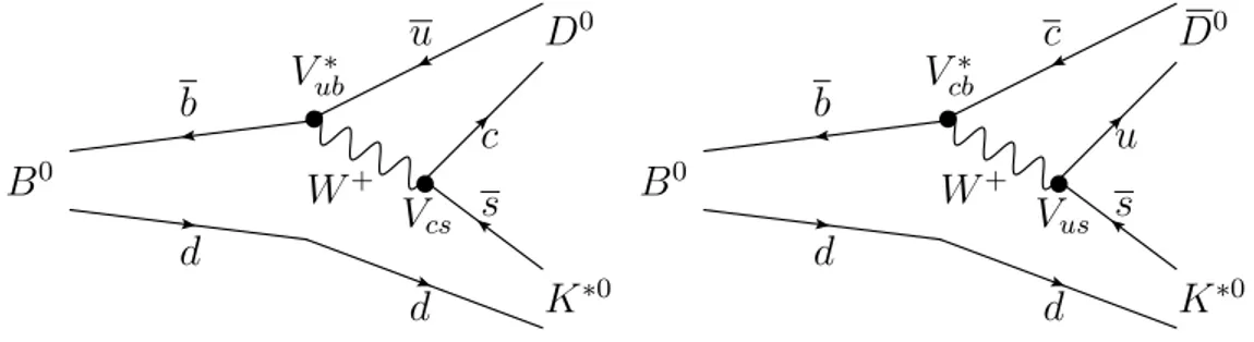
Measurements from the LHCb experiment yield γ = (74.0+5.0−5.8)◦ [4, 5], which is the most precise determination of γ from a single experiment. The precision is dominated by measurements exploiting the decay B+→ DK+, where D indicates a superposition of D0 and D0 mesons reconstructed in a final state common to both. In order to test internal consistency, and to improve overall sensitivity, it is important to complement these measurements with those based on other decay modes. One important example is B0 → DK∗0 [6], where K∗0 is the K∗(892)0 meson and is reconstructed in its decay to K+π−. This process involves the interference of B0 → D0K∗0 decays, which proceed via a b → c quark transition, and B0 → D0K∗0decays, which involve a b → u quark transition and are therefore suppressed relative to B0 → D0K∗0. Feynman diagrams of these decays are shown in Fig. 1. Both transitions are colour-suppressed, in contrast to the charged B-meson case where only the b → u transition is colour-suppressed. This leads to a greater suppression of the overall decay rates, but with the benefit of enhanced interference effects with respect to B+ → DK+ decays. The ratio rDK∗0
B between the magnitudes of the suppressed and favoured B0 decay amplitudes is expected to be around three times larger than the corresponding parameter in B+ → DK+ decays.
The LHCb collaboration has performed studies of B0 → DK∗0 decays using data corresponding to an integrated luminosity of 3.0 fb−1, reconstructing the D meson in the two-body final states K±π∓, K+K− and π+π− [7], and also the self-conjugate modes K0
Sπ+π
− and K0 SK+K
− [8, 9]. In addition, the two-body D decay modes K+π−, K+K−
B
0B
0b
b
d
d
d
d
u
c
s
c
u
s
D
0K
∗0D
0K
∗0W
+W
+V
ub∗ tV
cs tV
cb∗ tV
us tFigure 1: Feynman diagrams of (left) B0 → D0K∗0 and (right) B0 → D0K∗0.
1Except where stated otherwise, the inclusion of charge-conjugate processes is implied throughout
this paper.
and π+π− have previously been exploited in an amplitude analysis of B0 → DK+π− decays, including B0 → DK∗0 decays [10].
In this paper, results are presented for a study of B0 → DK∗0 decays performed on a data set corresponding to 3.0 fb−1 of integrated luminosity collected at centre-of-mass energies of 7 and 8 TeV during Run 1 of the LHC, and 1.8 fb−1 collected at 13 TeV during Run 2 in 2015 and 2016. Observables sensitive to γ are measured for the following final states of the D-meson decay: K±π∓, K+K−, π+π−, K±π∓π+π− and π+π−π+π−. The study of the two-body modes benefits from several improvements with respect to Ref. [7], as well as from the larger data set. The four-body modes are analysed for the first time in this decay chain. The measurements involving D → π+π−π+π− are based on Run 2 data alone, as the central processing that performs the first step of the selection did not include a suitable selection for this mode in Run 1.
The paper is organised as follows: Section 2 presents the observables to be measured, and their relationships to the physics parameters of interest; Sect. 3 discusses those aspects of the detector, trigger and simulation that are relevant for the measurement; Sects. 4, 5 and 6 describe the candidate selection, the fit of the mass spectra and the assignment of systematic uncertainties, respectively; the results, and their interpretation, are given in Sect. 7; and conclusions are presented in Sect. 8.
2
Analysis strategy
This analysis exploits the interference between B0 → D0K∗0 and B0 → D0K∗0 decays, with the D0 and D0 mesons reconstructed in a common final state. The partial widths of these decays are used to construct observables, which have a dependence on γ and the following parameters: the ratio rDK∗0
B between the magnitudes of the suppressed and favoured B0 decay amplitudes; the CP -conserving strong-phase difference δDK∗0
B between
the amplitudes; and a coherence factor κ, which accounts for other amplitudes that may contribute to the B0 → DK+π− final state in addition to the two diagrams responsible for the B0 → DK∗0 signal process. Detailed definitions of these parameters may be found in Ref. [7]. An amplitude analysis of B0 → DK+π− decays has determined the coherence factor to be κ = 0.958+0.005−0.046 for the K∗0 selection criteria used in this measurement (see Sect. 4) [10], which indicates an almost pure DK∗0 sample.
Reconstructing the charmed meson through a decay to a CP eigenstate, such as D → K+K− or D → π+π−, brings information on γ through a strategy first proposed by Gronau, London and Wyler (GLW) [11, 12]. The asymmetry
ACP ≡
Γ(B0 → DCPK∗0) − Γ(B0 → DCPK∗0) Γ(B0 → D
CPK∗0) + Γ(B0 → DCPK∗0)
, (1)
where Γ represents a partial decay width, is measured for both modes, yielding AKK
CP and
Aππ
CP, which are expected to be equal when the small CP -violating effects observed in the D-meson decay [13] are neglected; this assumption applies for the remainder of the discussion. The asymmetry is related to the underlying parameters through
ACP =
2κrDKB ∗0sin δBDK∗0sin γ RCP
where RCP is the charge-averaged rate of decays involving a D meson decaying to a CP eigenstate, defined as RCP ≡ 2 Γ(B0 → D CPK∗0) + Γ(B0 → DCPK∗0) Γ(B0 → D0K∗0) + Γ(B0 → D0K∗0) . (3) This is related to γ and the auxiliary parameters through
RCP = 1 + (rDK
∗0
B )
2
+ 2κrBDK∗0cos δDKB ∗0cos γ. (4) Experimentally it is convenient to access RCP by noting that it is closely approximated by
Rhh CP ≡ Γ(B0 → D(h+h−)K∗0) + Γ(B0 → D(h+h−)K∗0) Γ(B0 → D(K−π+)K∗0) + Γ(B0 → D(K+π−)K∗0) × B(D0 → K−π+) B(D0 → h+h−), (5) where the branching fractions B are known [14].
As proposed in Refs. [15, 16], multibody D-meson decays to self-conjugate final states may be used in a quasi-GLW analysis provided their fractional CP content is known. Hence the observables A4π
CP and R4πCP are measured, which are analogous to the two-body observables ACP and RhhCP, but for the decay D → π+π
−π+π−. These new observables can be interpreted through equivalent expressions to Eqs. 2 and 4 in which the interference terms acquire a factor of (2F4π
+ − 1), where F+4π is the fractional CP -even content of the decay, measured to be 0.769 ± 0.023 from quantum-correlated D-meson decays [17].
The decays D → K±π∓ are exploited in a method proposed by Atwood, Dunietz and Soni (ADS) [18, 19]. Considering the decays K∗0 → K+π− and K∗0→ K−π+, four categories are defined: two decays with the same charge of the final-state kaons, which are favoured and labelled Kπ, and two decays with the opposite charge of the final-state kaons, which are suppressed and labelled πK. The interference effects, and hence sensitivity to γ, are expected to be substantial for the suppressed modes, and smaller for the favoured modes.
The partial-rate asymmetry of the suppressed ADS decays is given by AπK
ADS ≡
Γ(B0 → D(π−K+)K∗0) − Γ(B0 → D(π+K−)K∗0)
Γ(B0 → D(π−K+)K∗0) + Γ(B0 → D(π+K−)K∗0), (6) and the charge-averaged rate with respect to the favoured modes by
RπK
ADS ≡
Γ(B0 → D(π−K+)K∗0) + Γ(B0 → D(π+K−)K∗0)
Γ(B0 → D(K−π+)K∗0) + Γ(B0 → D(K+π−)K∗0), (7) which have the following dependence on γ and the auxiliary parameters:
AπK ADS = 2κrDK∗0 B rKπD sin(δDK ∗0 B + δDKπ) sin γ (rDK∗0 B )2+ (rKπD )2+ 2κrDK ∗0 B rKπD cos(δDK ∗0 B + δKπD ) cos γ , (8) RπK ADS = (rDK∗0 B )2+ (rDKπ)2+ 2κrDK ∗0 B rDKπcos(δDK ∗0 B + δDKπ) cos γ 1 + (rDK∗0 B rDKπ)2+ 2κrDK ∗0 B rDKπcos(δDK ∗0 B + δDKπ) cos γ . (9)
Here, rKπ
D = 0.059 ± 0.001 is the ratio between the doubly Cabibbo-suppressed and Cabibbo-favoured decay amplitudes of the neutral charm meson, and δKπ
D = (192.1 + 8.6 −10.2)◦ is a strong-phase difference between the amplitudes [20].2
The quantities measured experimentally are the ratios RπK + = Γ(B0 → D(π+K−)K∗0) Γ(B0 → D(K+π−)K∗0) (10) and RπK− = Γ(B 0 → D(π−K+)K∗0) Γ(B0 → D(K−π+)K∗0). (11) The relationships AπK ADS ' (R πK − − RπK+ )/(R πK − + RπK+ ) (12) and RπK ADS ' (R πK + + R πK − )/2 (13)
allow the ADS observables to be recovered, where the approximate equalities are exact in the absence of CP asymmetry in the favoured modes.
The ADS method can be extended in an analogous way to the four-body mode D → K±π∓π+π−, with observables RπKππ
± . In interpreting the results it is necessary to account for the variation of amplitude across the phase space of the D-meson decay. In the equivalent relations for Eqs. 8 and 9 the amplitude ratio and charm strong-phase difference become rK3π
D and δK3πD , respectively, which are quantities averaged over phase space, and the interference terms [21] are multiplied by a coherence factor κK3π
D . These parameters have been measured in studies of charm mixing and quantum-correlated D-meson decays: rK3π D = 0.0549 ± 0.006, δK3πD = (128 +28 −17)◦ and κK3πD = 0.43 +0.17 −0.13 [22, 23]. In the favoured ADS modes the asymmetries
AKπ(ππ)ADS = Γ(B
0 → D(K−π+(π+π−))K∗0) − Γ(B0 → D(K+π−(π+π−))K∗0)
Γ(B0 → D(K−π+(π+π−))K∗0) + Γ(B0 → D(K+π−(π+π−))K∗0) (14) are measured. These modes are expected to exhibit much smaller CP asymmetries than the suppressed decay channels.
Observables associated with the decay B0
s → DK∗0 are also measured. This decay is expected to exhibit negligible CP violation, but serves as a useful control mode. In this case, for the ADS selection the final state with opposite-sign kaons constitutes the favoured mode, and so the analogously defined asymmetries AπK(ππ)s,ADS are measured. Signal yields are currently too small to permit a study of the suppressed mode. Finally, the GLW asymmetries AKK
s,CP, Aππs,CP and A4πs,CP, defined analogously to Eq. 1, and the ratios RKKs,CP, Rππ
s,CP and R4πs,CP, defined analogously to Eq. 5, are determined.
3
Detector, online selection and simulation
The LHCb detector [24, 25] is a single-arm forward spectrometer covering the pseudorapidity range 2 < η < 5, designed for the study of particles containing b or
2All expressions and charm strong-phase values are given in the convention CP |D0i = |D0i. This
implies a 180◦offset with respect to the values quoted in Ref. [20], which are defined with a different sign convention.
c quarks. The detector includes a high-precision tracking system consisting of a silicon-strip vertex detector surrounding the pp interaction region, a large-area silicon-silicon-strip detector located upstream of a dipole magnet with a bending power of about 4 Tm, and three stations of silicon-strip detectors and straw drift tubes placed downstream of the magnet. The tracking system provides a measurement of the momentum, p, of charged particles with a relative uncertainty that varies from 0.5% at low momentum to 1.0% at 200 GeV/c. The minimum distance of a track to a primary vertex (PV), the impact parameter (IP), is measured with a resolution of (15 + 29/pT) µm, where pT is the component of the momentum transverse to the beam, in GeV/c. Different types of charged hadrons are distinguished using information from two ring-imaging Cherenkov (RICH) detectors. Photons, electrons and hadrons are identified by a calorimeter system consisting of scintillating-pad and preshower detectors, an electromagnetic and a hadronic calorimeter. Muons are identified by a system composed of alternating layers of iron and multiwire proportional chambers.
The online event selection is performed by a trigger, which consists of a hardware stage, based on information from the calorimeter and muon systems, followed by a software stage, which applies a full event reconstruction. The events considered in the analysis must be triggered at the hardware level when either one of the final-state tracks of the signal decay deposits enough energy in the calorimeter system, or when one of the other tracks in the event, not reconstructed as part of the signal candidate, fulfils any trigger requirement. At the software stage, it is required that at least one particle should have high pT and high χ2IP, where χ2IP is defined as the difference in the PV fit χ2 with and without the inclusion of that particle. A multivariate algorithm [26] is used to identify secondary vertices consistent with being a two-, three- or four-track b-hadron decay. The PVs are fitted with and without the B candidate tracks, and the PV that gives the smallest χ2IP is associated with the B candidate.
Simulated events are used to describe the signal mass shapes and compute efficiencies. In the simulation, pp collisions are generated using Pythia [27] with a specific LHCb configuration [28]. Decays of hadronic particles are described by EvtGen [29], in which final-state radiation is generated using Photos [30]. The interaction of the generated particles with the detector, and its response, are implemented using the Geant4 toolkit [31] as described in Ref. [32].
4
Offline selection
Signal B-meson candidates are obtained by combining D and K∗0 candidates, and are required to have a pT greater than 5 GeV/c, a lifetime greater than 0.2 ps, and a good-quality vertex fit. The D candidate is reconstructed from the seven different decay modes of interest within a ±25 MeV/c2 window around the known D0 mass [14], and must have a pT greater than 1.8 GeV/c. The K∗0 candidate is reconstructed from the final state K+π−, selected within a ±50 MeV/c2 window around the known K∗0 mass and with a total pT of at least 1 GeV/c. This mass window is approximately the width of the K∗(892)0 resonance [14]. The helicity angle θ∗, defined as the angle between the K+ momentum in the K∗0 rest frame and the K∗0 momentum in the B0 rest frame, is required to satisfy |cos(θ∗)| > 0.4. This requirement removes 60% of the combinatorial background with a fake K∗0, while retaining 93% of the signal. The D and K∗0 candidates are both
required to have a good-quality vertex fit, a significant separation from the PV, and a distance-of-closest-approach between their decay products of less than 0.5 mm. All charged final-state particles are required to have a good-quality track fit, p greater than 1 GeV/c, and pT greater than 100 MeV/c. The B decay chain is refitted [33] with the D mass fixed to its known value and the B meson constrained to originate from its associated PV.
Gradient Boosted Decision Trees (BDTs) [34] are used to separate signal from combina-torial background. A shared BDT is employed for the favoured and suppressed two-body ADS modes, and similarly for the four-body ADS modes. Three independent BDTs are used to select the K+K−, π+π− and π+π−π+π− decays. All BDTs are trained with samples of simulated B0 → DK∗0 decays as signal and with candidates from the upper B mass sideband (5800 < m(B) < 6000 MeV/c2) in data as background. The discriminating variables in the BDT comprise: the B vertex-fit χ2; the χ2IP of the B and D candidates; the χ2IP and pT of the K∗0products; the angle between the B momentum vector and the vector between the PV and the B decay vertex; and the pT asymmetry between the B candidate and other tracks from the PV in a cone around the B candidate. The pT asymmetry is defined as (pBT − pcone
T )/(pBT + pconeT ), where pBT is the transverse momentum of the B candidate and pcone
T is the scalar sum of the transverse momenta of all other tracks in the cone. The radius of the cone is chosen to be 1.5 units in the plane of pseudorapidity and azimuthal angle (expressed in radians). The pT asymmetry is a measure of the isolation of the B candidate. The BDTs applied to B candidates with two-body D-meson decays also use the pT and χ2IP of the D decay products. These variables are not included in the BDTs applied to B candidates with four-body D decays to avoid significant changes to the phase-space distribution.
Particle-identification (PID) information from the RICH detectors is used to improve the purity of the different D-meson samples. Criteria are chosen such that no candidate can appear in more than one D decay category. A stringent PID requirement is applied to the kaon from the K∗0 candidate to suppress contamination from B0 → Dπ+π− decays, with a pion misidentified as a kaon.
It is possible for both the kaon and pion (or one of the two pions, in the four-body case) from the D-meson decay in the favoured mode to be misidentified, and thus pollute the suppressed sample. To eliminate this source of contamination, the D invariant mass is reconstructed with the opposite mass hypothesis for the kaon and pion. Candidates within ±15 MeV/c2 of the known D0 mass in this alternative reconstruction are vetoed. After this veto, a contamination rate of O(0.1%) is expected in the suppressed mode. No veto is applied to remove B0 → DK∗0 decays where both the kaon and pion from the K∗0 candidate are misidentified, as this background is sufficiently suppressed by the PID requirement on the kaon, leaving a contamination rate of O(0.7%) in the suppressed mode.
Additional background can arise from B0
(s) → D
−h+ (h = K, π), D−
sK+ or D+sπ− decays, with D±(s) decaying to a three-body combination of kaons and pions. This con-tamination is removed by imposing a ±15 MeV/c2 veto around the known D±
(s) mass in the invariant mass of the relevant three tracks. These vetoes are over 99% efficient at retaining signal candidates.
A background from charmless B decays that peaks at the same invariant mass as the signal is suppressed by requiring that the flight distance of the D candidate divided by its uncertainty be greater than 3. A further background from B+ → DK+ decays that
are mistakenly combined with a random pion from elsewhere in the event contaminates the region in invariant mass above the signal. This background is removed with a veto of ±25 MeV/c2 around the known B+ mass in the invariant mass of the D meson and the kaon from the K∗0 candidate.
5
Invariant-mass fit
The selected data set comprises two LHC runs and seven D-meson decay modes. The sample is further divided into B0 and B0 candidates, based on the charge of the kaon from the K∗0 meson. This gives a total of 26 categories, as the π+π−π+π− channel is not selected in the Run 1 data. The invariant-mass distributions are fit simultaneously in these categories with an unbinned extended maximum-likelihood fit. A fit model is developed comprising several signal and background components, which unless otherwise stated are modelled using simulated signal and background samples reconstructed as the signal decay and passing the selection requirements. The components are:
1. Signal B0 → DK∗0 and B0
s → DK∗0decays, described by Cruijff functions [35] with free means and widths, and tail parameters fixed from simulation.
2. Combinatorial background, described by an exponential function with a free slope. As the shape is completely free in the fit, no simulation is used to model this background.
3. Partially reconstructed background from B0 → D∗K∗0 and B0
s → D∗K∗0 decays, where D∗represents either a D∗0or D∗0meson. The D∗meson decays via D∗ → Dπ0 or D∗ → Dγ, where the neutral pion or photon is not reconstructed. These components are described by analytic probability distribution functions constructed from a parabolic function to describe the decay kinematics that is convolved with the sum of two Gaussians with a common mean to describe the detector resolution, as further described in Ref. [36]. All shape parameters are fixed from simulation. The form of the parabola depends on both the missed particle and the helicity of the D∗ meson, which can be equal to zero (longitudinal polarisation) or ±1 (transverse polarisation).
4. Partially reconstructed background from B+ → DK+π−π+ decays, where the π+ meson is not reconstructed. This background is described by the sum of two Gaussian functions with separate means and a parabola convolved with the sum of two Gaussians with a common mean. All shape parameters are fixed from simulation. 5. A background from B0 → Dπ+π− decays, with one of the pions misidentified as a
kaon. This background is described by the sum of two Crystal Ball functions [37] with all shape parameters fixed from simulation.
The signal and combinatorial background yields are free parameters for each LHC run. Preliminary studies showed that the ratios of the yields of the partially reconstructed backgrounds with respect to the signal yields are compatible within uncertainties between Runs 1 and 2, and so a single value is used in the fit. The same assumption cannot be made for the misidentified B0 → Dπ+π− background, as the yield of this background is
Table 1: Summary of signal yields. The uncertainties are statistical.
Decay channel B0 yield B0 yield
B0 → D(K+K− )K∗0 67 ± 10 77 ± 11 B0 → D(π+π−)K∗0 27 ± 6 40 ± 7 B0 → D(π+π−π+π−)K∗0 32 ± 7 35 ± 8 B0 → D(K+π− )K∗0 786 ± 29 754 ± 29 B0 → D(π+K−)K∗0 76 ± 16 47 ± 15 B0 → D(K+π−π+π−)K∗0 557 ± 25 548 ± 25 B0 → D(π+K−π+π−)K∗0 41 ± 14 40 ± 14
affected by the π → K misidentification rate, which can vary between running periods. The proportion of this background with respect to the signal is therefore corrected in Run 2 with respect to Run 1. Studies of simulated signal and background samples determine this correction factor to be 0.928 ± 0.014.
The B0 → Dπ+π−background is assumed to have no CP asymmetry, as the candidates cannot be tagged as coming from a B0 or B0 decay, and the difference between the π+ and π− misidentification rates is found to be negligible in simulated samples. Misidentified B0 → Dπ+π− decays should therefore contaminate B0 and B0 equally. The B0
s → D
∗K∗0 background is not expected to exhibit CP violation, so the CP asymmetry is fixed to zero in the GLW modes but is free in the ADS modes. The yields of the B0 → Dπ+π− and B0
s → D
∗K∗0 backgrounds are free parameters in the ADS modes and fixed in the GLW modes relative to the ADS yields from knowledge of the D0 branching fractions [14] and relative selection efficiencies determined from simulation. The B0 → D∗K∗0 background may exhibit CP violation, so the yields of each D decay channel are free parameters, thus allowing for a nonzero CP asymmetry. The relative yields and asymmetries of the B+ → DK+π−π+ background are fixed using measurements from Ref. [38].
For both the B0 → D∗K∗0 and B0
s → D
∗K∗0 backgrounds, the relative proportion of partially reconstructed D∗ → Dγ and D∗ → Dπ0 decays is fixed by known D∗0 branching fractions [14] and relative selection efficiency as determined from simulation. The fraction of longitudinal polarisation is unknown and is therefore a free parameter in the fit.
Figures 2 to 5 show the invariant mass distributions and the fitted shapes for the various components. Table 1 gives the signal yields for each D final state. The fit strategy is validated by pseudoexperiments, and is found to be reliable and unbiased for all free parameters.
The observables introduced in Sect. 2 are determined directly from the fit. The ratios and asymmetries between the raw yields are corrected for efficiency differences, and production and detection asymmetries. To obtain the ratios RhhCP and R4πCP, the raw ratios are normalised using the corresponding D0 branching fractions. These corrections are discussed further in Sect. 6.
6
Correction factors and systematic uncertainties
The measured observables are either asymmetries or ratios of yields between similar final states, and are thus robust against systematic biases. Nonetheless, small differences in
] 2 c ) [MeV/ *0 K D ] KK ([ m 5000 5200 5400 5600 5800 ) 2 c Candidates / (16 MeV/ 20 40 60 80 100 120 Data Fit Combinatorial *0 K D → 0 B *0 K D → s 0 B − π + π − K D → − B *0 K * D → s 0 B − π + π D → 0 B *0 K * D → 0 B LHCb ] 2 c ) [MeV/ *0 K D ] KK ([ m 5000 5200 5400 5600 5800 ) 2 c Candidates / (16 MeV/ 20 40 60 80 100 120 Data Fit Combinatorial *0 K D → 0 B *0 K D → s 0 B + π − π + K D → + B *0 K * D → s 0 B − π + π D → 0 B *0 K * D → 0 B LHCb ] 2 c ) [MeV/ *0 K D ] π π ([ m 5000 5200 5400 5600 5800 ) 2 c Candidates / (16 MeV/ 5 10 15 20 25 30 35 40 Data Fit Combinatorial *0 K D → 0 B *0 K D → s 0 B − π + π − K D → − B *0 K * D → s 0 B − π + π D → 0 B *0 K * D → 0 B LHCb ] 2 c ) [MeV/ *0 K D ] π π ([ m 5000 5200 5400 5600 5800 ) 2 c Candidates / (16 MeV/ 5 10 15 20 25 30 35 40 Data Fit Combinatorial *0 K D → 0 B *0 K D → s 0 B + π − π + K D → + B *0 K * D → s 0 B − π + π D → 0 B *0 K * D → 0 B LHCb
Figure 2: Invariant-mass distributions (data points with error bars) and results of the fit (lines and coloured areas) for the two-body GLW modes (top left) B0→ D(K+K−)K∗0, (top right) B0 →
D(K+K−)K∗0, (bottom left) B0 → D(π+π−)K∗0 and (bottom right) B0 → D(π+π−)K∗0.
efficiencies between numerator and denominator mean that correction factors must be applied to the ratios, apart from the case of RπK(ππ)± where an identical selection is used for both the suppressed and favoured ADS modes. The selection efficiencies are computed from simulated signal samples, which are weighted in the transverse momentum and pseudorapidity of the B meson to agree with the data distributions. The efficiencies of the PID requirements between different charges and D final states are evaluated using calibration samples, which are weighted to match the momentum and pseudorapidity of the simulated signal samples. Uncertainties are assigned due to the finite size of the simulated samples, and for possible biases introduced by the binning schemes used in the reweighting of the calibration sample and the background-subtraction procedure used for these samples.
As can be seen from Eq. 5, determining Rhh
CP requires normalising the measured ratio of yields by a ratio of D0 branching fractions. These branching fractions are taken from Ref. [14] and the uncertainties are propagated to the observables.
The raw observables are corrected for detection asymmetry, which is predominantly caused by the shorter interaction length of K− mesons compared with K+ mesons. The difference between the kaon and pion detection asymmetries, AD(K−π+), is computed following the method used in Ref. [39]. Raw charge asymmetries Araw(K−π+π+) and Araw(K0π+) are measured for the decays D+→ K−π+π+ and D+ → K0π+, respectively. These asymmetries are determined using calibration samples which are weighted to match the kinematics of the kaons and pions in the signal data set. The value of AD(K−π+) is
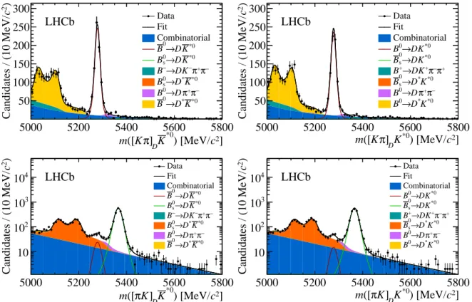
] 2 c ) [MeV/ *0 K D ] π K ([ m 5000 5200 5400 5600 5800 ) 2 c Candidates / (10 MeV/ 50 100 150 200 250 300 Data Fit Combinatorial *0 K D → 0 B *0 K D → s 0 B − π + π − K D → − B *0 K * D → s 0 B − π + π D → 0 B *0 K * D → 0 B LHCb ] 2 c ) [MeV/ *0 K D ] π K ([ m 5000 5200 5400 5600 5800 ) 2 c Candidates / (10 MeV/ 50 100 150 200 250 300 Data Fit Combinatorial *0 K D → 0 B *0 K D → s 0 B + π − π + K D → + B *0 K * D → s 0 B − π + π D → 0 B *0 K * D → 0 B LHCb ] 2 c ) [MeV/ *0 K D ] K π ([ m 5000 5200 5400 5600 5800 ) 2 c Candidates / (10 MeV/ 10 2 10 3 10 4 10 Data Fit Combinatorial *0 K D → 0 B *0 K D → s 0 B − π + π − K D → − B *0 K * D → s 0 B − π + π D → 0 B *0 K * D → 0 B LHCb ] 2 c ) [MeV/ *0 K D ] K π ([ m 5000 5200 5400 5600 5800 ) 2 c Candidates / (10 MeV/ 10 2 10 3 10 4 10 Data Fit Combinatorial *0 K D → 0 B *0 K D → s 0 B + π − π + K D → + B *0 K * D → s 0 B − π + π D → 0 B *0 K * D → 0 B LHCb
Figure 3: Invariant-mass distributions (data points with error bars) and results of the fit (lines and coloured areas) for the two-body ADS modes (top left) B0→ D(K−π+)K∗0, (top right) B0 → D(K+π−)K∗0, (bottom left) B0 → D(π−K+)K∗0 and (bottom right) B0 → D(π+K−)K∗0.
The bottom distributions are shown on a logarithmic scale.
] 2 c ) [MeV/ *0 K D ] π π π π ([ m 5000 5200 5400 5600 5800 ) 2 c Candidates / (16 MeV/ 5 10 15 20 25 30 35 40 45 Data Fit Combinatorial *0 K D → 0 B *0 K D → s 0 B − π + π − K D → − B *0 K * D → s 0 B − π + π D → 0 B *0 K * D → 0 B LHCb ] 2 c ) [MeV/ *0 K D ] π π π π ([ m 5000 5200 5400 5600 5800 ) 2 c Candidates / (16 MeV/ 5 10 15 20 25 30 35 40 45 Data Fit Combinatorial *0 K D → 0 B *0 K D → s 0 B + π − π + K D → + B *0 K * D → s 0 B − π + π D → 0 B *0 K * D → 0 B LHCb
Figure 4: Invariant-mass distributions (data points with error bars) and results of the fit (lines and coloured areas) for the four-body GLW mode (left) B0 → D(π+π−π+π−)K∗0, (right)
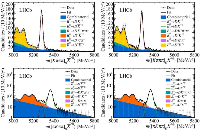
] 2 c ) [MeV/ *0 K D ] π π π K ([ m 5000 5200 5400 5600 5800 ) 2 c Candidates / (10 MeV/ 20 40 60 80 100 120 140 160 180 200 Data Fit Combinatorial *0 K D → 0 B *0 K D → s 0 B − π + π − K D → − B *0 K * D → s 0 B − π + π D → 0 B *0 K * D → 0 B LHCb ] 2 c ) [MeV/ *0 K D ] π π π K ([ m 5000 5200 5400 5600 5800 ) 2 c Candidates / (10 MeV/ 20 40 60 80 100 120 140 160 180 200 Data Fit Combinatorial *0 K D → 0 B *0 K D → s 0 B + π − π + K D → + B *0 K * D → s 0 B − π + π D → 0 B *0 K * D → 0 B LHCb ] 2 c ) [MeV/ *0 K D ] π π K π ([ m 5000 5200 5400 5600 5800 ) 2 c Candidates / (10 MeV/ 1 10 2 10 3 10 4 10 DataFit Combinatorial *0 K D → 0 B *0 K D → s 0 B − π + π − K D → − B *0 K * D → s 0 B − π + π D → 0 B *0 K * D → 0 B LHCb ] 2 c ) [MeV/ *0 K D ] π π K π ([ m 5000 5200 5400 5600 5800 ) 2 c Candidates / (10 MeV/ 1 10 2 10 3 10 4 10 DataFit Combinatorial *0 K D → 0 B *0 K D → s 0 B + π − π + K D → + B *0 K * D → s 0 B − π + π D → 0 B *0 K * D → 0 B LHCb
Figure 5: Invariant-mass distributions (data points with error bars) and results of the fit (lines and coloured areas) for the four-body ADS modes (top left) B0 → D(K−π+π−π+)K∗0, (top right) B0 → D(K+π−π+π−)K∗0, (bottom left) B0 → D(π−K+π+π−)K∗0 and (bottom right)
B0 → D(π+K−π−π+)K∗0. The bottom distributions are shown on a logarithmic scale.
calculated from AD(K−π+) = Araw(K−π+π+) − Araw(K0π+) + AD(K0), where AD(K0) is the measured value of the detection asymmetry in the decay K0 → π+π−, giving AD(K−π+) = (−0.92 ± 0.20)% in Run 1 and (−1.0 ± 0.6)% in Run 2. A correction of AD(K−π+) is applied to the observables for each K±π∓ pair in the final state.
The observables are also corrected for the asymmetry in the production of B0 and B0 mesons within the acceptance of the analysis, Aprod. This asymmetry has been measured in bins of B-meson momentum and pseudorapidity in Run 1 [40]. A weighted average based on the kinematical distributions of simulated signal gives Aprod= (−0.8 ± 0.5)%. The same central value is applied for Run 2, with the uncertainty doubled in order to account for a possible change in asymmetry due to the higher collision energy.
Uncertainties are assigned to account for the shape parameters that are fixed in the invariant-mass model. The values of these fixed parameters derive from fits to simulated samples, and so the uncertainties on these fits are propagated to the mass model. The fixed tail parameters of the signal shape are treated as a single source of systematic uncertainty. Uncertainties due to all fixed parameters related to the background shapes are treated simultaneously, apart from those for the partially reconstructed B0
s → D
∗K∗0 decays, which are an important source of background that overlaps with the signal region, and are therefore treated separately.
Uncertainties are also considered for other fixed parameters in the fit. These are the relative proportion of partially reconstructed D∗ → Dπ0 and D∗ → Dγ decays, the
correction to the relative yield of misidentified B0 → Dπ+π− decays between Run 1 and Run 2, and the relative yields and CP asymmetries of the partially reconstructed B+ → DK+π−π+ background. For the latter, the uncertainties taken from Ref. [38] are doubled to account for the fact that there are possible differences in the phase-space acceptance between the two analyses.
A study of the invariant-mass sidebands of the D candidates is performed in order to search for evidence of any residual charmless background which would also contaminate the B signal region. This sideband study is performed after imposing the flight distance cut on the D candidate, but without applying the BDT selection, as this may not have a uniform acceptance in D mass. Regions of the sidebands where there are known reflections from D-meson decays with misidentified final products are excluded. No significant signals are found from charmless decays in any mode. The measured yields are extrapolated into the signal region and taken as the central values from which many pseudoexperiments with an added charmless background component are simulated. These data sets are fitted using the nominal fit model which neglects the new background contribution, and a systematic uncertainty is assigned based on the measured bias.
Table 2 gives the systematic uncertainties for each observable. Systematic uncertainties which are more than two orders of magnitude smaller than the statistical uncertainty are considered to be negligible and ignored. The non-negligible uncertainties are added in quadrature to give the total systematic uncertainty, which in all cases is considerably smaller than the statistical uncertainty.
The acceptance for the four-body D-decay modes is not fully uniform across phase space. Studies performed with amplitude models of these decays indicate that, at the current level of sensitivity, a nonuniform acceptance does not lead to any significant bias when the observables are interpreted in terms of γ and the other underlying physics parameters. No systematic uncertainty is assigned.
7
Results and discussion
The measured values for the principal observables are AKK CP = −0.05 ± 0.10 ± 0.01, Aππ CP = −0.18 ± 0.14 ± 0.01, RKK CP = 0.92 ± 0.10 ± 0.02, Rππ CP = 1.32 ± 0.19 ± 0.03, A4π CP = −0.03 ± 0.15 ± 0.01, R4π CP = 1.01 ± 0.16 ± 0.04, RπK + = 0.064 ± 0.021 ± 0.002, RπK − = 0.095 ± 0.021 ± 0.003, RπKππ + = 0.074 ± 0.026 ± 0.002, RπKππ − = 0.072 ± 0.025 ± 0.003, AKπ ADS = 0.047 ± 0.027 ± 0.010, AKπππ ADS = 0.037 ± 0.032 ± 0.010,
where the first uncertainty is statistical, and the second systematic. The values of RπK ± and RπKππ± are used to calculate the suppressed-mode ADS observables, which are found to be
T able 2: S yste matic uncertain ties for the observ ables. Uncertain ties are sho wn if they are larger than 1% of the statistical uncertain ty . The total systematic uncertain ty is c al c u late d b y summing all sources in quadr ature. Statistical uncertain ties are giv en for reference. Source A K K C P A π π C P R K K C P R π π C P A 4 π C P R 4 π CP R π K + R π K − R π K π π + R π K π π − A K π ADS A K π π π ADS Selection efficie n c y -0.008 0.011 -0.012 -PID efficiency 0.002 -0.004 0.004 0.002 0.007 -0.002 0.003 Branc hing ratios -0.017 0.025 -0.031 -Pro duction asymmetry 0.006 0.006 -0.010 -0.006 0.006 Detection asymm etry 0.004 0.004 0.004 0.007 0.007 0.007 < 0 .001 < 0 .001 < 0 .001 < 0 .001 0.008 0.008 Signal shap e parameters -< 0 .001 < 0 .001 < 0 .001 < 0 .001 -B 0 s→ D ∗ K ∗ 0 shap e parameters -0.001 -< 0 .001 < 0 .001 < 0 .001 < 0 .001 -Other bac kground shap e parameters -0.003 -0.003 < 0 .001 0.001 0.001 0.002 -D ∗ → D 0 γ /π 0 inputs -0.002 -0.002 0.002 0.002 0.002 0.002 -B → D π π PID correction -0.006 -< 0 .001 < 0 .001 -< 0 .001 B → D K π π inputs -0.001 0.002 -0.002 -Charmless bac kgroun d 0.003 0.002 -0.003 0.004 0.011 < 0 .001 < 0 .001 -< 0 .001 0.002 0.001 T otal systematic 0.008 0. 008 0.020 0.029 0.014 0.037 0.002 0.003 0.002 0.003 0.010 0.010 Statistical 0.10 0.14 0.10 0.19 0.15 0.16 0.021 0.021 0.026 0.025 0.027 0.032
AπK ADS = 0.19 ± 0.19 ± 0.01, RπK ADS = 0.080 ± 0.015 ± 0.002, AπKππ ADS = −0.01 ± 0.24 ± 0.01, RπKππ ADS = 0.073 ± 0.018 ± 0.002.
All CP asymmetries are compatible with zero to within two standard deviations. The values of the GLW asymmetries and ratios are found to be consistent between the two modes, within 0.8 and 1.8 standard deviations, respectively. The results for D → π+π−π+π− are in agreement with these values, after correcting for the known CP -even content of this state. The same observables determined for B0
s decays are compatible with the CP -conserving hypothesis. Results for B0
s decays can be found in Appendix A, together with the results for all observables separated between the Run 1 and Run 2 data sets, and full correlation matrices.
The statistical significances of the signal yields in the previously unobserved channels are calculated using Wilks’ theorem [41]. The likelihood profiles are convolved with a Gaussian function with standard deviation equal to the systematic uncertainties on the yields. This procedure yields a significance of 8.4σ for the B0 → D(π+π−π+π−)K∗0 decay, 5.8σ for the B0 → D(π+K−)K∗0 decay and 4.4σ for the B0 → D(π+K−π+π−)K∗0 decay, constituting the first observation of the first two modes, and strong evidence for the presence of the suppressed four-body ADS channel.
The results are interpreted in terms of the underlying physics parameters γ, rDKB ∗0 and δDK∗0
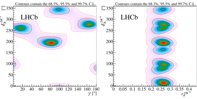
B by performing a global χ2 minimisation. The minimised χ2/ndf is equal to 7.1/9. A scan of physics parameters is performed for a range of values and the difference in χ2 between the parameter scan and the global minimum, ∆χ2, is evaluated. The confidence level for any pair of parameters is calculated assuming that these are normally distributed, which allows the ∆χ2 = 2.30, 6.18, 11.8 contours to be drawn, corresponding to 68.6%, 95.5%, 99.7% confidence levels, respectively. These contours are shown in Fig. 6. As expected, there is a degeneracy in the (γ, δDK∗0
B ) plane. Four favoured solutions can be seen, two of which are compatible with the existing LHCb determination of γ [4, 5], which is dominated by results obtained from B+→ DK+ processes, which have values of rDK− B and δDK − B different from rDK ∗0 B and δDK ∗0
B . The degeneracy of the solutions can be broken by combining these results with those using other D decay modes, specifically the D → KS0π+π− decay. The value of rBDK∗0 is determined to be 0.265 ± 0.023. In accordance with expectation, this is almost a factor of three larger than the corresponding parameter in B+ → DK+ decays [4, 5]. This measurement is consistent with, and more accurate than, the previous measurement by LHCb in Ref. [7].
] ° [ γ 20 40 60 80 100 120 140 160 180 ] ° [ *0 DK B δ 0 50 100 150 200 250 300 350
LHCb
Contours contain the 68.3%, 95.5% and 99.7% C.L.
*0 DK B r 0 0.05 0.1 0.15 0.2 0.25 0.3 0.35 0.4 ] ° [ *0 DK B δ 0 50 100 150 200 250 300 350
LHCb
Contours contain the 68.3%, 95.5% and 99.7% C.L.
Figure 6: Contour plots showing 2D scans of (left) δBDK∗0 versus γ and (right) δBDK∗0 versus rBDK∗0. The lines represent the ∆χ2 = 2.30, 6.18 and 11.8 contours, corresponding to 68.6%, 95.5% and 99.7% confidence levels (C.L.), respectively.
8
Conclusion
Measurements of CP observables in B0 → DK∗0 decays with the D meson decaying to K+π−, π+K−, K+K− and π+π− are performed using LHCb data collected in 2011, 2012, 2015 and 2016. The results, benefitting from the increased data sample and improved analysis methods, supersede those of the previous study [7]. Measurements with D mesons reconstructed in the K+π−π+π−, π+K−π+π− and π+π−π+π− final states are presented for the first time. First observations are obtained for the suppressed ADS mode B0 → D(π+K−)K∗0 and the mode B0 → D(π+π−π+π−)K∗0.
The observables are interpreted in terms of the weak phase γ and associated parameters, and are found to be compatible with the previous LHCb results [4,5], which are dominated by measurements of B+ → DK+ processes. The amplitude ratio rDK∗0
B is determined to be equal to 0.265 ± 0.023 at a confidence level of 68.3%. These results can be combined with those from other modes in B0 → DK∗0 decays to provide powerful constraints on γ. This can be compared to results obtained from studies of other processes.
Acknowledgements
We express our gratitude to our colleagues in the CERN accelerator departments for the excellent performance of the LHC. We thank the technical and administrative staff at the LHCb institutes. We acknowledge support from CERN and from the national agencies: CAPES, CNPq, FAPERJ and FINEP (Brazil); MOST and NSFC (China); CNRS/IN2P3 (France); BMBF, DFG and MPG (Germany); INFN (Italy); NWO (Netherlands); MNiSW and NCN (Poland); MEN/IFA (Romania); MSHE (Russia); MinECo (Spain); SNSF and SER (Switzerland); NASU (Ukraine); STFC (United Kingdom); DOE NP and NSF (USA). We acknowledge the computing resources that are provided by CERN, IN2P3 (France),
KIT and DESY (Germany), INFN (Italy), SURF (Netherlands), PIC (Spain), GridPP (United Kingdom), RRCKI and Yandex LLC (Russia), CSCS (Switzerland), IFIN-HH (Romania), CBPF (Brazil), PL-GRID (Poland) and OSC (USA). We are indebted to the communities behind the multiple open-source software packages on which we depend. Individual groups or members have received support from AvH Foundation (Germany); EPLANET, Marie Sk lodowska-Curie Actions and ERC (European Union); ANR, Labex P2IO and OCEVU, and R´egion Auvergne-Rhˆone-Alpes (France); Key Research Program of Frontier Sciences of CAS, CAS PIFI, and the Thousand Talents Program (China); RFBR, RSF and Yandex LLC (Russia); GVA, XuntaGal and GENCAT (Spain); the Royal Society and the Leverhulme Trust (United Kingdom).
Appendices
A
Additional results
Observables for B0s → DK∗0 decays are defined analogously to those for B0 → DK∗0 decays in Eqs. 1, 5 and 14. The measured observables are
AπK s,ADS = 0.006 ± 0.017 ± 0.012, AπKππ s,ADS = −0.007 ± 0.021 ± 0.013, AKK s,CP = 0.06 ± 0.05 ± 0.01, Aππ s,CP = −0.11 ± 0.09 ± 0.01, RKK s,CP = 1.06 ± 0.06 ± 0.02, Rππ s,CP = 1.05 ± 0.10 ± 0.02, A4π s,CP = 0.12 ± 0.08 ± 0.02, R4π s,CP = 0.964 ± 0.086 ± 0.031. The B0 and B0
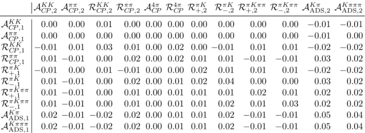
s observables are also measured separately for Run 1 and Run 2; these measurements are presented in Table 3. The correlation matrices for the principal observables are given in Tables 4, 5 and 6 for the combined, Run 1, and Run 2 results, respectively. Table 7 gives the correlations between the Run 1 and Run 2 results.
Table 3: Measured observables split by LHC running period. Observables relating to B0 →
D(π+π−π+π−)K∗0 decays are not presented for Run 1, as this decay channel was not selected in the Run 1 data.
Run 1 Run 2 AKK CP −0.19 ± 0.16 ± 0.01 0.05 ± 0.13 ± 0.02 Aππ CP −0.06 ± 0.23 ± 0.01 −0.26 ± 0.18 ± 0.01 RKK CP 0.93 ± 0.15 ± 0.02 0.91 ± 0.13 ± 0.02 Rππ CP 1.39 ± 0.33 ± 0.04 1.27 ± 0.24 ± 0.03 A4π CP — −0.03 ± 0.15 ± 0.01 R4π CP — 1.01 ± 0.16 ± 0.04 RπK + 0.045 ± 0.032 ± 0.003 0.076 ± 0.027 ± 0.003 RπK − 0.120 ± 0.035 ± 0.003 0.080 ± 0.025 ± 0.003 RπKππ + 0.12 ± 0.04 ± 0.00 0.047 ± 0.031 ± 0.003 RπKππ − 0.099 ± 0.043 ± 0.004 0.056 ± 0.029 ± 0.003 AKπ ADS 0.03 ± 0.04 ± 0.01 0.055 ± 0.035 ± 0.016 AKπππ ADS 0.03 ± 0.05 ± 0.01 0.042 ± 0.040 ± 0.016 AπK s,ADS 0.011 ± 0.027 ± 0.010 0.002 ± 0.022 ± 0.019 AπKππ s,ADS −0.042 ± 0.035 ± 0.012 0.012 ± 0.026 ± 0.020 AKK s,CP −0.03 ± 0.08 ± 0.01 0.13 ± 0.07 ± 0.02 Aππ s,CP −0.06 ± 0.17 ± 0.01 −0.13 ± 0.11 ± 0.02 RKK s,CP 1.14 ± 0.09 ± 0.03 1.01 ± 0.07 ± 0.02 Rππ s,CP 0.83 ± 0.15 ± 0.02 1.22 ± 0.14 ± 0.03 A4π s,CP — 0.12 ± 0.08 ± 0.02 R4π s,CP — 0.96 ± 0.09 ± 0.03
Table 4: Combined statistical and systematic correlation matrix for the principal observables. AKK CP AππCP RKKCP RππCP A4πCP R4πCP RπK+ RπK− RπKππ+ RπKππ− AKπADS AKπππADS AKK CP 1.00 0.00 0.03 −0.01 0.00 0.00 0.00 −0.01 −0.01 −0.01 −0.01 −0.01 Aππ CP 0.00 1.00 0.01 0.06 0.00 0.00 0.00 0.00 0.00 0.00 −0.01 −0.01 RKK CP 0.03 0.01 1.00 0.04 0.00 0.03 0.02 0.02 0.00 0.00 −0.04 −0.03 Rππ CP −0.01 0.06 0.04 1.00 0.00 0.04 0.01 0.03 0.02 0.02 0.03 0.03 A4π CP 0.00 0.00 0.00 0.00 1.00 0.01 0.00 0.00 0.00 0.00 0.00 0.00 R4π CP 0.00 0.00 0.03 0.04 0.01 1.00 0.01 0.02 0.02 0.03 0.02 0.01 RπK + 0.00 0.00 0.02 0.01 0.00 0.01 1.00 0.05 0.01 0.01 0.08 0.00 RπK − −0.01 0.00 0.02 0.03 0.00 0.02 0.05 1.00 0.02 0.02 −0.08 0.03 RπKππ + −0.01 0.00 0.00 0.02 0.00 0.02 0.01 0.02 1.00 0.06 0.02 0.11 RπKππ − −0.01 0.00 0.00 0.02 0.00 0.03 0.01 0.02 0.06 1.00 0.03 −0.06 AKπ ADS −0.01 −0.01 −0.04 0.03 0.00 0.02 0.08 −0.08 0.02 0.03 1.00 0.08 AKπππ ADS −0.01 −0.01 −0.03 0.03 0.00 0.01 0.00 0.03 0.11 −0.06 0.08 1.00
Table 5: Combined statistical and systematic correlation matrix for the principal observables in Run 1 data only.
AKK CP ,1 AππCP ,1 RKKCP ,1 RππCP ,1 RπK+,1 RπK−,1 RπKππ+,1 RπKππ−,1 AKπADS,1 AKπππADS,1 AKK CP ,1 1.00 0.00 0.08 0.00 0.00 0.00 0.00 0.00 −0.01 −0.01 Aππ CP ,1 0.00 1.00 0.00 0.01 0.00 0.00 0.00 0.00 0.00 0.00 RKK CP ,1 0.08 0.00 1.00 0.03 0.01 0.02 0.00 0.00 −0.02 −0.01 Rππ CP ,1 0.00 0.01 0.03 1.00 0.00 0.03 0.01 0.01 0.01 0.01 RπK +,1 0.00 0.00 0.01 0.00 1.00 0.02 0.00 0.00 0.05 −0.01 RπK −,1 0.00 0.00 0.02 0.03 0.02 1.00 0.01 0.01 −0.13 0.01 RπKππ +,1 0.00 0.00 0.00 0.01 0.00 0.01 1.00 0.04 0.01 0.15 RπKππ −,1 0.00 0.00 0.00 0.01 0.00 0.01 0.04 1.00 0.01 −0.11 AKπ ADS,1 −0.01 0.00 −0.02 0.01 0.05 −0.13 0.01 0.01 1.00 0.02 AKπππ ADS,1 −0.01 0.00 −0.01 0.01 −0.01 0.01 0.15 −0.11 0.02 1.00
Table 6: Combined statistical and systematic correlation matrix for the principal observables in Run 2 data only.
AKK CP ,2 AππCP ,2 RKKCP ,2 RππCP ,2 A4πCP ,2 R4πCP ,2 RπK+,2 RπK−,2 RπKππ+,2 RπKππ−,2 AKπADS,2 AKπππADS,2 AKK CP ,2 1.00 −0.01 −0.01 0.01 0.00 0.01 0.01 0.01 −0.01 −0.01 0.04 0.03 Aππ CP ,2 −0.01 1.00 0.01 0.08 0.00 0.00 −0.01 −0.01 0.01 0.01 −0.02 −0.01 RKK CP ,2 −0.01 0.01 1.00 0.03 0.00 0.03 0.01 0.01 0.01 0.01 −0.04 −0.03 Rππ CP ,2 0.01 0.08 0.03 1.00 0.00 0.03 0.02 0.03 −0.01 0.00 0.03 0.03 A4π CP ,2 0.00 0.00 0.00 0.00 1.00 0.00 0.00 0.00 0.00 0.00 0.00 0.01 R4π CP ,2 0.01 0.00 0.03 0.03 0.00 1.00 0.01 0.01 0.00 0.01 0.01 0.01 RπK +,2 0.01 −0.01 0.01 0.02 0.00 0.01 1.00 0.05 0.00 0.00 0.12 0.02 RπK −,2 0.01 −0.01 0.01 0.03 0.00 0.01 0.05 1.00 0.00 0.00 −0.07 0.02 RπKππ +,2 −0.01 0.01 0.01 −0.01 0.00 0.00 0.00 0.00 1.00 0.05 −0.02 0.04 RπKππ −,2 −0.01 0.01 0.01 0.00 0.00 0.01 0.00 0.00 0.05 1.00 −0.02 −0.09 AKπ ADS,2 0.04 −0.02 −0.04 0.03 0.00 0.01 0.12 −0.07 −0.02 −0.02 1.00 0.10 AKπππ ADS,2 0.03 −0.01 −0.03 0.03 0.01 0.01 0.02 0.02 0.04 −0.09 0.10 1.00
Table 7: Correlation matrix for the principal observables between Run 1 and Run 2 data. AKK CP ,2 A ππ CP ,2 R KK CP ,2 R ππ CP ,2 A 4π CP R 4π CP R πK +,2 RπK−,2 RπKππ+,2 RπKππ−,2 AKπADS,2 A Kπππ ADS,2 AKK CP ,1 0.00 0.00 0.01 0.00 0.00 0.00 0.00 0.00 0.00 0.00 −0.01 −0.01 Aππ CP ,1 0.00 0.00 0.00 0.00 0.00 0.00 0.00 0.00 0.00 0.00 −0.01 0.00 RKK CP ,1 −0.01 0.01 0.03 0.01 0.00 0.02 0.00 −0.01 0.01 0.01 −0.02 −0.02 Rππ CP ,1 0.01 −0.01 0.00 0.02 0.00 0.02 0.01 0.01 −0.01 −0.01 0.03 0.02 RπK +,1 −0.01 0.00 0.01 −0.01 0.00 0.00 0.02 0.01 0.01 0.01 −0.02 −0.02 RπK −,1 0.01 −0.01 0.00 0.02 0.00 0.01 0.02 0.04 0.00 0.00 0.03 0.02 RπKππ +,1 0.01 −0.01 0.00 0.01 0.00 0.01 0.01 0.01 0.02 0.01 0.02 0.02 RπKππ −,1 0.01 −0.01 0.00 0.01 0.00 0.01 0.01 0.02 0.01 0.03 0.02 0.02 AKπ ADS,1 0.02 −0.01 −0.02 0.02 0.00 0.01 0.01 0.02 −0.01 −0.01 0.05 0.04 AKπππ ADS,1 0.02 −0.01 −0.02 0.02 0.00 0.01 0.01 0.02 −0.01 −0.01 0.05 0.04
References
[1] N. Cabibbo, Unitary symmetry and leptonic decays, Phys. Rev. Lett. 10 (1963) 531. [2] M. Kobayashi and T. Maskawa, CP -violation in the renormalizable theory of weak
interaction, Prog. Theor. Phys. 49 (1973) 652.
[3] L. Wolfenstein, Parametrization of the Kobayashi–Maskawa matrix, Phys. Rev. Lett. 51 (1983) 1945.
[4] LHCb collaboration, Update of the LHCb combination of the CKM angle γ using B → DK decays, LHCb-CONF-2018-002, 2018.
[5] LHCb collaboration, R. Aaij et al., Measurement of the CKM angle γ from a combi-nation of LHCb results, JHEP 12 (2016) 087, arXiv:1611.03076.
[6] I. Dunietz, CP violation with self-tagging Bd modes, Phys. Lett. B270 (1991) 75. [7] LHCb collaboration, R. Aaij et al., Measurement of CP violation parameters in
B0→ DK∗0 decays, Phys. Rev. D90 (2014) 112002, arXiv:1407.8136.
[8] LHCb collaboration, R. Aaij et al., Model-independent measurement of the CKM angle γ using B0→ DK∗0 decays with D → K0
Sπ+π
− and K0 SK+K
−, JHEP 06 (2016) 131, arXiv:1604.01525.
[9] LHCb collaboration, R. Aaij et al., Measurement of the CKM angle γ using B0→ DK∗0 with D → K0
Sπ+π
− decays, JHEP 08 (2016) 137, arXiv:1605.01082. [10] LHCb collaboration, R. Aaij et al., Constraints on the unitarity triangle angle γ
from Dalitz plot analysis of B0→ DK+π− decays, Phys. Rev. D93 (2016) 112018, Erratum ibid. D94 (2016) 079902, arXiv:1602.03455.
[11] M. Gronau and D. Wyler, On determining a weak phase from charged B decay asymmetries, Phys. Lett. B265 (1991) 172.
[12] M. Gronau and D. London, How to determine all the angles of the unitarity triangle from Bd0 → DKS and Bs0 → Dφ, Phys. Lett. B253 (1991) 483.
[13] LHCb collaboration, R. Aaij et al., Observation of CP violation in charm decays, Phys. Rev. Lett. 122 (2019) 211803, arXiv:1903.08726.
[14] Particle Data Group, M. Tanabashi et al., Review of particle physics, Phys. Rev. D98 (2018) 030001.
[15] M. Nayak et al., First determination of the CP content of D → π+π−π0 and D → K+K−π0, Phys. Lett. B740 (2015) 1, arXiv:1410.3964.
[16] S. Malde et al., First determination of the CP content of D → π+π−π+π− and updated determination of the CP contents of D → π+π−π0 and D → K+K−π0, Phys. Lett. B747 (2015) 9, arXiv:1504.05878.
[17] S. Harnew et al., Model-independent determination of the strong phase differ-ence between D0 and D0 → π+π−π+π− amplitudes, JHEP 01 (2018) 144, arXiv:1709.03467.
[18] D. Atwood, I. Dunietz, and A. Soni, Enhanced CP violation with B → KD0(D0) modes and extraction of the Cabibbo–Kobayashi–Maskawa angle γ, Phys. Rev. Lett. 78 (1997) 3257, arXiv:hep-ph/9612433.
[19] D. Atwood, I. Dunietz, and A. Soni, Improved methods for observing CP violation in B± → KD and measuring the CKM phase γ, Phys. Rev. D63 (2001) 036005, arXiv:hep-ph/0008090.
[20] Heavy Flavor Averaging Group, Y. Amhis et al., Averages of b-hadron, c-hadron, and τ -lepton properties as of summer 2016, Eur. Phys. J. C77 (2017) 895, arXiv:1612.07233, updated results and plots available at
https://hflav.web.cern.ch.
[21] D. Atwood and A. Soni, Role of a charm factory in extracting CKM-phase information via B → DK, Phys. Rev. D68 (2003) 033003, arXiv:hep-ph/0304085.
[22] LHCb collaboration, R. Aaij et al., First observation of D0–D0 oscillations in D0→ K+π+π−π− decays and a measurement of the associated coherence param-eters, Phys. Rev. Lett. 116 (2016) 241801, arXiv:1602.07224.
[23] T. Evans et al., Improved determination of the D → K−π+π+π− coherence factor and associated hadronic parameters from a combination of e+e− → ψ(3770) → c¯c and pp → c¯cX data, Phys. Lett. B757 (2016) 520, Erratum ibid. B765 (2017) 402, arXiv:1602.07430.
[24] LHCb collaboration, A. A. Alves Jr. et al., The LHCb detector at the LHC, JINST 3 (2008) S08005.
[25] LHCb collaboration, R. Aaij et al., LHCb detector performance, Int. J. Mod. Phys. A30 (2015) 1530022, arXiv:1412.6352.
[26] V. V. Gligorov and M. Williams, Efficient, reliable and fast high-level triggering using a bonsai boosted decision tree, JINST 8 (2013) P02013, arXiv:1210.6861.
[27] T. Sj¨ostrand, S. Mrenna, and P. Skands, A brief introduction to PYTHIA 8.1, Comput. Phys. Commun. 178 (2008) 852, arXiv:0710.3820.
[28] I. Belyaev et al., Handling of the generation of primary events in Gauss, the LHCb simulation framework, J. Phys. Conf. Ser. 331 (2011) 032047.
[29] D. J. Lange, The EvtGen particle decay simulation package, Nucl. Instrum. Meth. A462 (2001) 152.
[30] P. Golonka and Z. Was, PHOTOS Monte Carlo: A precision tool for QED corrections in Z and W decays, Eur. Phys. J. C45 (2006) 97, arXiv:hep-ph/0506026.
[31] Geant4 collaboration, J. Allison et al., Geant4 developments and applications, IEEE Trans. Nucl. Sci. 53 (2006) 270; Geant4 collaboration, S. Agostinelli et al., Geant4: A simulation toolkit, Nucl. Instrum. Meth. A506 (2003) 250.
[32] M. Clemencic et al., The LHCb simulation application, Gauss: Design, evolution and experience, J. Phys. Conf. Ser. 331 (2011) 032023.
[33] W. D. Hulsbergen, Decay chain fitting with a Kalman filter, Nucl. Instrum. Meth. A552 (2005) 566, arXiv:physics/0503191.
[34] L. Breiman, J. H. Friedman, R. A. Olshen, and C. J. Stone, Classification and regression trees, Wadsworth international group, Belmont, California, USA, 1984. [35] BaBar collaboration, P. del Amo Sanchez et al., Study of B → Xγ decays and
determination of |Vtd/Vts|, Phys. Rev. D82 (2010) 051101, arXiv:1005.4087. [36] LHCb collaboration, R. Aaij et al., Measurement of CP observables in B±→ D(∗)K±
and B±→ D(∗)π± decays, Phys. Lett. B777 (2017) 16, arXiv:1708.06370.
[37] T. Skwarnicki, A study of the radiative cascade transitions between the Upsilon-prime and Upsilon resonances, PhD thesis, Institute of Nuclear Physics, Krakow, 1986, DESY-F31-86-02.
[38] LHCb collaboration, R. Aaij et al., Study of B−→ DK−π+π− and B−→ Dπ−π+π− decays and determination of the CKM angle γ, Phys. Rev. D92 (2015) 112005, arXiv:1505.07044.
[39] LHCb collaboration, R. Aaij et al., Measurement of CP asymmetry in D0→ K−K+ and D0→ π−π+ decays, JHEP 07 (2014) 041, arXiv:1405.2797.
[40] LHCb collaboration, R. Aaij et al., Measurement of B0, B0
s, B+ and Λ0b production asymmetries in 7 and 8 TeV proton-proton collisions, Phys. Lett. B774 (2017) 139, arXiv:1703.08464.
[41] S. S. Wilks, The large-sample distribution of the likelihood ratio for testing composite hypotheses, Ann. Math. Stat. 9 (1938) 60.
LHCb collaboration
R. Aaij29, C. Abell´an Beteta46, B. Adeva43, M. Adinolfi50, C.A. Aidala78, Z. Ajaltouni7, S. Akar61, P. Albicocco20, J. Albrecht12, F. Alessio44, M. Alexander55, A. Alfonso Albero42, G. Alkhazov35, P. Alvarez Cartelle57, A.A. Alves Jr43, S. Amato2, Y. Amhis9, L. An19,
L. Anderlini19, G. Andreassi45, M. Andreotti18, J.E. Andrews62, F. Archilli20, J. Arnau Romeu8, A. Artamonov41, M. Artuso64, K. Arzymatov39, E. Aslanides8, M. Atzeni46, B. Audurier24, S. Bachmann14, J.J. Back52, S. Baker57, V. Balagura9,b, W. Baldini18,44, A. Baranov39, R.J. Barlow58, S. Barsuk9, W. Barter57, M. Bartolini21, F. Baryshnikov74, V. Batozskaya33, B. Batsukh64, A. Battig12, V. Battista45, A. Bay45, F. Bedeschi26, I. Bediaga1, A. Beiter64, L.J. Bel29, V. Belavin39, S. Belin24, N. Beliy4, V. Bellee45, K. Belous41, I. Belyaev36, G. Bencivenni20, E. Ben-Haim10, S. Benson29, S. Beranek11, A. Berezhnoy37, R. Bernet46, D. Berninghoff14, E. Bertholet10, A. Bertolin25, C. Betancourt46, F. Betti17,e, M.O. Bettler51, Ia. Bezshyiko46, S. Bhasin50, J. Bhom31, M.S. Bieker12, S. Bifani49, P. Billoir10, A. Birnkraut12, A. Bizzeti19,u, M. Bjørn59, M.P. Blago44, T. Blake52, F. Blanc45, S. Blusk64, D. Bobulska55, V. Bocci28, O. Boente Garcia43, T. Boettcher60, A. Boldyrev75, A. Bondar40,x, N. Bondar35, S. Borghi58,44, M. Borisyak39, M. Borsato14, M. Boubdir11, T.J.V. Bowcock56, C. Bozzi18,44, S. Braun14, A. Brea Rodriguez43, M. Brodski44, J. Brodzicka31, A. Brossa Gonzalo52, D. Brundu24,44, E. Buchanan50, A. Buonaura46, C. Burr58, A. Bursche24, J.S. Butter29, J. Buytaert44, W. Byczynski44, S. Cadeddu24, H. Cai68, R. Calabrese18,g, S. Cali20, R. Calladine49, M. Calvi22,i, M. Calvo Gomez42,m, A. Camboni42,m, P. Campana20, D.H. Campora Perez44, L. Capriotti17,e, A. Carbone17,e, G. Carboni27, R. Cardinale21,
A. Cardini24, P. Carniti22,i, K. Carvalho Akiba2, A. Casais Vidal43, G. Casse56, M. Cattaneo44, G. Cavallero21, R. Cenci26,p, M.G. Chapman50, M. Charles10,44, Ph. Charpentier44,
G. Chatzikonstantinidis49, M. Chefdeville6, V. Chekalina39, C. Chen3, S. Chen24, S.-G. Chitic44,
V. Chobanova43, M. Chrzaszcz44, A. Chubykin35, P. Ciambrone20, X. Cid Vidal43, G. Ciezarek44, F. Cindolo17, P.E.L. Clarke54, M. Clemencic44, H.V. Cliff51, J. Closier44, J.L. Cobbledick58, V. Coco44, J.A.B. Coelho9, J. Cogan8, E. Cogneras7, L. Cojocariu34,
P. Collins44, T. Colombo44, A. Comerma-Montells14, A. Contu24, N. Cooke49, G. Coombs44, S. Coquereau42, G. Corti44, C.M. Costa Sobral52, B. Couturier44, G.A. Cowan54, D.C. Craik60, A. Crocombe52, M. Cruz Torres1, R. Currie54, C.L. Da Silva63, E. Dall’Occo29, J. Dalseno43,v,
C. D’Ambrosio44, A. Danilina36, P. d’Argent14, A. Davis58, O. De Aguiar Francisco44,
K. De Bruyn44, S. De Capua58, M. De Cian45, J.M. De Miranda1, L. De Paula2, M. De Serio16,d, P. De Simone20, J.A. de Vries29, C.T. Dean55, W. Dean78, D. Decamp6, L. Del Buono10, B. Delaney51, H.-P. Dembinski13, M. Demmer12, A. Dendek32, V. Denysenko46, D. Derkach75, O. Deschamps7, F. Desse9, F. Dettori24, B. Dey69, A. Di Canto44, P. Di Nezza20, S. Didenko74, H. Dijkstra44, F. Dordei24, M. Dorigo26,y, A.C. dos Reis1, A. Dosil Su´arez43, L. Douglas55, A. Dovbnya47, K. Dreimanis56, L. Dufour44, G. Dujany10, P. Durante44, J.M. Durham63, D. Dutta58, R. Dzhelyadin41,†, M. Dziewiecki14, A. Dziurda31, A. Dzyuba35, S. Easo53,
U. Egede57, V. Egorychev36, S. Eidelman40,x, S. Eisenhardt54, U. Eitschberger12, R. Ekelhof12, S. Ek-In45, L. Eklund55, S. Ely64, A. Ene34, S. Escher11, S. Esen29, T. Evans61, A. Falabella17, C. F¨arber44, N. Farley49, S. Farry56, D. Fazzini9, M. F´eo44, P. Fernandez Declara44,
A. Fernandez Prieto43, F. Ferrari17,e, L. Ferreira Lopes45, F. Ferreira Rodrigues2,
S. Ferreres Sole29, M. Ferro-Luzzi44, S. Filippov38, R.A. Fini16, M. Fiorini18,g, M. Firlej32, C. Fitzpatrick44, T. Fiutowski32, F. Fleuret9,b, M. Fontana44, F. Fontanelli21,h, R. Forty44, V. Franco Lima56, M. Franco Sevilla62, M. Frank44, C. Frei44, J. Fu23,q, W. Funk44, E. Gabriel54, A. Gallas Torreira43, D. Galli17,e, S. Gallorini25, S. Gambetta54, Y. Gan3, M. Gandelman2, P. Gandini23, Y. Gao3, L.M. Garcia Martin77, J. Garc´ıa Pardi˜nas46, B. Garcia Plana43, J. Garra Tico51, L. Garrido42, D. Gascon42, C. Gaspar44, G. Gazzoni7, D. Gerick14, E. Gersabeck58, M. Gersabeck58, T. Gershon52, D. Gerstel8, Ph. Ghez6,