HAL Id: hal-00533205
https://hal.archives-ouvertes.fr/hal-00533205
Submitted on 21 Dec 2015
HAL is a multi-disciplinary open access
archive for the deposit and dissemination of
sci-entific research documents, whether they are
pub-lished or not. The documents may come from
teaching and research institutions in France or
abroad, or from public or private research centers.
L’archive ouverte pluridisciplinaire HAL, est
destinée au dépôt et à la diffusion de documents
scientifiques de niveau recherche, publiés ou non,
émanant des établissements d’enseignement et de
recherche français ou étrangers, des laboratoires
publics ou privés.
troposphere during July 2008 as seen from models,
satellite, and aircraft observations
H. Sodemann, Matthieu Pommier, S. R. Arnold, S. A. Monks, K. Stebel, J. F.
Burkhart, J. W. Hair, G. S. Diskin, Cathy Clerbaux, Pierre-François Coheur,
et al.
To cite this version:
H. Sodemann, Matthieu Pommier, S. R. Arnold, S. A. Monks, K. Stebel, et al.. Episodes of
cross-polar transport in the Arctic troposphere during July 2008 as seen from models, satellite, and
air-craft observations. Atmospheric Chemistry and Physics, European Geosciences Union, 2011, 11 (8),
pp.3631-3651. �10.5194/acp-11-3631-2011�. �hal-00533205�
www.atmos-chem-phys.net/11/3631/2011/ doi:10.5194/acp-11-3631-2011
© Author(s) 2011. CC Attribution 3.0 License.
Chemistry
and Physics
Episodes of cross-polar transport in the Arctic troposphere during
July 2008 as seen from models, satellite, and aircraft observations
H. Sodemann1, M. Pommier2, S. R. Arnold3, S. A. Monks3, K. Stebel1, J. F. Burkhart1, J. W. Hair4, G. S. Diskin4,
C. Clerbaux2,5, P.-F. Coheur5, D. Hurtmans5, H. Schlager6, A.-M. Blechschmidt7, J. E. Kristj´ansson7, and A. Stohl1
1Norwegian Institute for Air Research (NILU), Kjeller, Norway
2UPMC Univ. Paris 06, Universit´e Versailles St-Quentin, CNRS/INSU, LATMOS-IPSL, Paris, France
3Institute for Climate and Atmospheric Science, School of Earth and Environment, University of Leeds, Leeds, UK 4Atmospheric Sciences, NASA Langley Research Center, Hampton, Virginia, USA
5Spectroscopie de l’Atmosph`ere, Chimie Quantique et Photophysique, Universit´e Libre de Bruxelles, Brussels, Belgium 6Deutsches Zentrum f¨ur Luft- und Raumfahrt, Institut f¨ur Physik der Atmosph¨are, Oberpfaffenhofen, Germany
7Department of Geosciences, University of Oslo, Oslo, Norway
Received: 22 October 2010 – Published in Atmos. Chem. Phys. Discuss.: 5 November 2010 Revised: 25 March 2011 – Accepted: 29 March 2011 – Published: 19 April 2011
Abstract. During the POLARCAT summer campaign in
2008, two episodes (2–5 July and 7–10 July 2008) occurred where low-pressure systems traveled from Siberia across the Arctic Ocean towards the North Pole. The two cyclones had extensive smoke plumes from Siberian forest fires and an-thropogenic sources in East Asia embedded in their asso-ciated air masses, creating an excellent opportunity to use satellite and aircraft observations to validate the performance of atmospheric transport models in the Arctic, which is a challenging model domain due to numerical and other com-plications.
Here we compare transport simulations of carbon monox-ide (CO) from the Lagrangian transport model FLEXPART and the Eulerian chemical transport model TOMCAT with retrievals of total column CO from the IASI passive infrared sensor onboard the MetOp-A satellite. The main aspect of the comparison is how realistic horizontal and vertical struc-tures are represented in the model simulations. Analysis of CALIPSO lidar curtains and in situ aircraft measurements provide further independent reference points to assess how reliable the model simulations are and what the main limita-tions are.
The horizontal structure of mid-latitude pollution plumes agrees well between the IASI total column CO and the model simulations. However, finer-scale structures are too quickly
Correspondence to: H. Sodemann
(hso@nilu.no)
diffused in the Eulerian model. Applying the IASI averag-ing kernels to the model data is essential for a meanaverag-ingful comparison. Using aircraft data as a reference suggests that the satellite data are biased high, while TOMCAT is biased low. FLEXPART fits the aircraft data rather well, but due to added background concentrations the simulation is not in-dependent from observations. The multi-data, multi-model approach allows separating the influences of meteorological fields, model realisation, and grid type on the plume struc-ture. In addition to the very good agreement between sim-ulated and observed total column CO fields, the results also highlight the difficulty to identify a data set that most realis-tically represents the actual pollution state of the Arctic at-mosphere.
1 Introduction
The polar regions of the northern hemisphere are often per-ceived as remote and pristine. However, atmospheric trans-port can swiftly bring pollution from emission sources at lower latitudes to the Arctic. Until recently, it was a com-monly accepted view that air pollution continuously seeps into the Arctic, similar to a bathtub filling up slowly from a dripping faucet (Raatz and Shaw, 1984; Barrie, 1986). Re-cent research has replaced this concept by a picture where synoptic-scale events lead to the rapid advection of polluted mid-latitude air that is subsequently assimilated into the cold
Arctic air mass through radiative cooling (Stohl, 2006). One implication of the dripping faucet hypothesis was the view of the Arctic as a more or less homogeneous, well-mixed air mass with so-called background levels of atmospheric pollu-tants. Observations from aircraft and more recently aerosol lidar have however demonstrated repeatedly since the 1980s that the stably stratified Arctic air mass consists of an inho-mogeneous, finely stirred m´elange of layered air masses with different physical and chemical properties that only slowly undergoes mixing (Engvall et al., 2008, 2009).
The reason for the fine layering of the Arctic atmosphere lies in its thermal stratification. The lower part of the Arctic troposphere, the so-called polar dome, is isolated from the rest of the atmosphere due to its low potential temperatures (Klonecki et al., 2003; Stohl, 2006). Towards its southern boundaries this cold airmass creates an apparent horizontal transport barrier, which enhances the concentration gradients between the mid-latitudes and the Arctic. It should be noted that while to a first order the Arctic front apparently hinders pollution transport into the Arctic (Barrie, 1986) it is also the region of baroclinic development that ultimately leads to the poleward advection of mid-latitude air as part of frontal systems. Within the Arctic dome, transport and exchange are particularly slow and long residence times ensue. As air masses move towards the pole they are radiatively cooled, and become incorporated into a region of large vertical gra-dient of potential temperature. Layers of different age and origin are stacked on top of one another and are only slowly incorporated into the Arctic dome by further radiative cool-ing, mixing and diffusion. In contrast, above the polar dome residence times can be on the order of only a few days (Klo-necki et al., 2003; Stohl, 2006).
The fine-scale structure of the Arctic atmosphere poses a major problem for atmospheric transport model simulations. Computational constraints require that Eulerian grid mod-els are commonly run at horizontal and vertical resolutions that are inadequate for representing the actual structure of the Arctic atmosphere. This leads to the overly rapid dif-fusion and decay along the boundaries of advected plumes (Rastigejev et al., 2010). Another common problem in Eu-lerian models using a latitude-longitude grid is that the con-vergence of the meridians towards the poles leads to a sin-gularity that needs to be accommodated by specific numer-ics. While in most models measures are taken to ensure nu-merical stability near the pole, such as decreasing the grid resolution, subdividing the time step (Krol et al., 2005) or changing the advection scheme around the pole, side-effects like reduced effective resolution or enhanced numerical dif-fusion cannot be avoided. These side-effects counteract the requirement that numerical diffusion should be small to re-tain the sharp gradients in stable air masses (Krol et al., 2005). Other approaches such as calculations on an icosa-hedral grid are not yet widely used (Thuburn, 1997). An-other common approach to atmospheric transport modeling is Lagrangian modelling. Lagrangian transport models
cal-culate the advection of individual air parcels based on three-dimensional wind fields. A major advantage of these models is that in principle they are not limited by grid resolution. Unlike Eulerian chemistry transport models (CTMs), most Lagrangian models are currently not capable of simulating the chemical transformation of an air mass. Also, due to is-sues with mass distribution, Eulerian models are so far better suited to perform global budget studies and simulations over long timescales. To some extent, Lagrangian models may also be affected by numerical problems near the pole as the meteorological data which force them are calculated by Eu-lerian models. The long transport pathways, long lifetimes of pollutants in the cold Arctic air, and strong vertical temper-ature gradients close to the surface (Strunin et al., 1997) are further challenges for all atmospheric transport calculations in polar regions. To our knowledge, simulations of transport in the Arctic atmosphere from both model types have not yet been compared directly.
In addition to numerical difficulties, simulations in the Arctic are restricted by the sparsity of observational data. Routine meteorological surface observations for example that are assimilated into meteorological data used by trans-port model simulations are less dense in the Arctic. Fur-thermore, it is difficult to obtain reliable data for validating model simulations in this region. Passive and active remote sensing, for example from satellites, is hampered by low so-lar zenith angles and the reflective and thermal properties of the surface (Turquety et al., 2009). Another difficulty is that emission sources are mostly located far outside the Arc-tic, and are often not well quantified. Most of the emission sources that affect the Arctic are located in Europe, Eurasia and other mid-latitude areas (Stohl, 2006). The source region influence is subject to a pronounced seasonal cycle. During winter, emissions from fossil fuel and biofuel combustion and industrial processes constitute the main sources. Dur-ing sprDur-ing and summer pollution sources are forest fires and other biomass burning as well as industrial emissions (Stohl et al., 2007; Warneke et al., 2009; Paris et al., 2009; Warneke et al., 2010).
Taking technical and observational problems together, it is not surprising that a recent inter-comparison study between 17 CTMs for the Arctic mainly highlighted the disagreement between model results, e.g. with respect to the simulated seasonal cycle of atmospheric constituents (Shindell et al., 2008). Models also disagree on the role and distance of pol-lution sources. While Koch and Hansen (2005) argued for a large contribution from South Asia to black carbon con-centrations in the Arctic, Stohl (2006) emphasized the much larger importance of mid-latitude sources. Resolving such discrepancies is scientifically important but also relevant for creating effective measures to control Arctic pollution levels. The IPY (International Polar Year) placed a large observa-tional and model focus on the polar regions during the years 2007–2009. During the international POLARCAT GRACE summer campaign in July 2008 a range of data from different
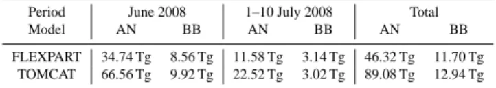
Table 1. Anthropogenic (AN) and biomass-burning (BB) CO emis-sions during 1 June–10 July 2008 in the FLEXPART and TOMCAT models. Accounting of biomass-burning CO emissions is restricted
to 15◦N for both models. FLEXPART anthropogenic emissions
exclude South America, Africa and Oceania (∼20% of the global emissions). AN emissions in the TOMCAT model also include nat-ural emissions from the POET inventory which are not related to fire.
Period June 2008 1–10 July 2008 Total Model AN BB AN BB AN BB FLEXPART 34.74 Tg 8.56 Tg 11.58 Tg 3.14 Tg 46.32 Tg 11.70 Tg
TOMCAT 66.56 Tg 9.92 Tg 22.52 Tg 3.02 Tg 89.08 Tg 12.94 Tg
platforms were acquired which created an excellent opportu-nity for an in-depth model-to-data comparison study in the Arctic. During the period 2–10 July 2008 two low-pressure systems moved from Siberia towards the North Pole, one of them even towards Europe, bringing along extensive smoke plumes from biomass burning in Siberia embedded in the as-sociated air masses. The chemical composition of the air masses was measured from aircraft, and observed by active and passive remote sensing instruments from satellite and air-craft platforms.
The aim of this paper is to evaluate to what extent the transport across the pole in terms of the horizontal and ver-tical structure of air masses is simulated realisver-tically by an Eulerian and a Lagrangian transport model. It is not our aim to decide which model is performing better, but rather to gain a complementary view from the two types of models. Nev-ertheless we do aim to point out which aspects of the simu-lations, according to the observations, are reliable and which may be affected by artifacts. In-situ and remote sensing data acquired during the period 2–10 July 2008 are used for ref-erence and validation. In addition, the paper highlights the difficulties in comparing data sets from such distinct sources as models, satellites, and aircraft.
2 Models and data
This study is primarily based on the simulation results of two atmospheric transport models: (i) the Lagrangian par-ticle dispersion model FLEXPART (Stohl et al., 2005) and (ii) the Eulerian CTM TOMCAT (Arnold et al., 2005; Chip-perfield, 2006). An important distinction between FLEX-PART and TOMCAT is that TOMCAT includes a complete set of chemical reactions in the atmosphere, while in FLEX-PART only some removal mechanisms are parameterised. We mainly focus on carbon monoxide (CO) in our compari-son, as it is typically associated with anthropogenic and bio-genic combustion fumes and is hence useful as a tracer for atmospheric pollution transport. Furthermore, CO is observ-able by satellite and aircraft, and its atmospheric lifetime in the Arctic during summer is assumed to be sufficiently long
(2–4 weeks) for long-range transport to play an important role.
2.1 Lagrangian model FLEXPART
The Lagrangian particle dispersion model FLEXPART was run based on meteorological fields from the ECMWF (Euro-pean Centre for Medium-Range Weather Forecasts) analyses at 0.5◦×0.5◦resolution. Six-hourly analysis data were sup-plemented by 3-h forecast data to increase the time resolution of the meteorological fields. FLEXPART advects hypotheti-cal air parcels of equal mass based on the interpolated three-dimensional wind fields and additional random motions that account for turbulence and convection. North of 86◦N, a grid in polar stereographic projection was used to avoid a numeri-cal singularity at the pole. Output data from the FLEXPART calculations were stored at 0.5◦×0.5◦ horizontal resolution and on 15 vertical levels.
Emissions from biomass burning were initialized from daily MODIS fire hot-spot data. The fire emissions scaled according to land-use classes were distributed in the lower 150 m of the atmosphere. Agricultural fires were assumed to have burned during daytime only, while other fires burned for 24 h (Stohl et al., 2007). Total CO emissions from nat-ural and anthropogenic sources (excluding South America, Africa and Oceania) during June and 1–10 July are listed in Table 1. The model simulation was run with a CO gas tracer and a black carbon (BC) aerosol tracer. Air parcels of both tracers were removed from the simulation after a life-time of 20 days, assuming that by then the air parcels become in-corporated into the so-called atmospheric background (see Sect. 2.5). No chemical production/destruction of CO was considered, in particular, CO was not removed by oxidation with the OH radical. BC aerosol tracer was removed by wet and dry deposition processes (Stohl et al., 2005). Anthro-pogenic emissions of CO and BC were initialised from the updated EDGAR 3.2 emissions inventory for the year 2000 (Olivier and Berdowski, 2001).
2.2 Eulerian model TOMCAT
The TOMCAT model is a three-dimensional Eulerian CTM and has been previously used for a number of atmospheric chemistry transport simulations (Arnold et al., 2005; Chip-perfield, 2006). The model is forced using 6-hourly ECMWF operational analyses of wind speed, temperature and hu-midity. The model was run at a horizontal resolution of 2.8◦×2.8◦ with 31 vertical levels up to 10 hPa.
Large-scale advection is implemented using the Prather (1986) scheme. The model accounts for sub-grid scale transport using the Tiedtke (1989) convection scheme and the Holt-slag and Boville (1993) parameterization for turbulent mix-ing in the boundary layer followmix-ing the method of Wang et al. (1999). The emissions have been updated for the purpose of this study to provide the best available estimate for 2008.
Monthly averaged anthropogenic and ship emissions are taken from Streets’ v1.2 ARCTAS emission inventory (avail-able from http://www.cgrer.uiowa.edu/arctas/emission.html) with volatile organic compound speciation applied follow-ing Lamarque et al. (2010). Isoprene and methanol emis-sions were calculated using the MEGAN model (Guenther et al., 2006) and all other natural emissions are taken from the POET inventories, as used in the MOZART-4 model, described in Emmons et al. (2010). Note that emissions in July are generally lower than during other months of a year. Nevertheless, emissions used for TOMCAT are higher than the yearly emissions from EDGAR used in the FLEXPART model, as all global emission sources are considered (Ta-ble 1). Daily biomass burning emissions estimates of trace gases were compiled specifically for 2008 for the ARCTAS campaign. These were created using MODIS satellite re-trievals of hot-spots, area burned estimates and fuel loadings (Wiedinmyer et al., 2006). These daily emission fluxes are regridded to the TOMCAT grid and emitted every timestep and distributed throughout the lowest level gridbox (up to
∼113 m) (Monks et al., 2011).
The Gaussian grid used in TOMCAT uses a constant lon-gitude space and has a box “edge” at the pole. Consequently, there are a couple of polar transport issues which need to be overcome. For E-W advection the decreasing size of the boxes near the pole means that transport in this direction could violate the Courant-Friedrichs-Levy (CFL) criterion, which specifies that the wind speed for a given timestep and grid size cannot exceed a certain value in order to maintain numerical stability. Typically, the grid box size has to be increased or the timestep decreased to overcome this prob-lem. TOMCAT groups boxes together for the E-W transport to form an “extended polar zone” following the method de-scribed in Prather et al. (1987). For the model resolution and timestep used in this study this occurs at gridpoints pole-ward of 78◦and effectively reduces the model resolution at the pole. For the N-S transport the model uses a full normal grid. However, at the pole there is a singularity (i.e. the box edges have zero size) and the model has an explicit treatment to advect mass from a box to the one diametrically oppo-site depending on the wind vector at the pole. This allows cross polar transport to be considered in the N-S direction. E-W transport in the last latitude band will also contribute to cross polar transport within the limitation of the model res-olution. As the Prather (1986) scheme advects second-order moments (gradient and curvature) of the tracer field along with the mixing ratios, some of the finer-scale structure is retained once a feature has passed over the pole and is dis-tributed over a larger number of gridboxes. Earlier versions of the TOMCAT/SLIMCAT model have been widely used for studies of stratospheric polar ozone and shown very good agreement with observations (Chipperfield et al., 2005).
2.3 Satellite remote-sensing data
Total column atmospheric CO observations (TCO) retrieved by the IASI instrument are used to assess the horizontal accu-racy of the model simulations. IASI is an infrared sounder on board of the polar-orbiting Metop-A satellite, providing mea-surements of trace gases such as CO, O3, CH4, HNO3, SO2
and H2O (Clerbaux et al., 2009). It provides near-global
cov-erage twice per day on a 98.7◦-inclination sun-synchronous polar orbit at about 817 km altitude. The local solar time at equator crossing is about 09:30 (ascending node) with a 29-day repeat cycle. Daylight data over land contain more information on the CO vertical distribution than night data over oceans, because of the impact of thermal contrast (the temperature difference between the ground and the first at-mospheric layer) that limits the vertical sensitivity (Turquety et al., 2009). For this study we only used daylight obser-vations, i.e. where the zenith angle was lower or equal to 83◦. IASI has a horizontal coverage with a swath of around 2200 km. Each atmospheric view consists of 2×2 pixels, each with a 12 km pixel diameter and spaced out 50 km at nadir. The CO data were retrieved from IASI radiance spec-tra using the FORLI-CO software developed at the Universit´e Libre de Bruxelles. The employed algorithm is based on the optimal estimation method (Rodgers, 2000) as described in Turquety et al. (2009) and George et al. (2009). CO obser-vations from the IASI instrument have been evaluated in an Arctic environment and were found to provide meaningful results (Pommier et al., 2010).
Since the satellite observations from IASI are not equally sensitive to all atmospheric layers, for a fair comparison the model data had to be weighted with the IASI averaging ker-nel (AK). This is essentially the same as creating an artificial satellite retrieval from the model data. A mean AK for each day and each 1◦ latitude-longitude position has been used, created by averaging the individual AKs from the respec-tive IASI daytime observations (Fig. 1a). Using a local daily mean AK introduces small random errors to the data analy-sis. To calculate simulated total column retrievals, data from both models have then been weighted using the equation
yo=Ak·ym+(I − Ak) ·ya (1)
where yois the simulated satellite retrieval, Akis the IASI
AK vector for a column, ymis a model data vector, I is the
identity matrix, and ya is the IASI a priori (Rodgers, 2000;
George et al., 2009).
The Cloud-Aerosol Lidar with Orthogonal Polarization (CALIOP) is in orbit on board of the CALIPSO satellite as part of the NASA A-Train suite of satellites (Winker et al., 2009). CALIPSO was launched in 2006, and flies at 705 km altitude in a 98.2◦-inclination sun-synchronous polar orbit. The equator-crossing time is at 10:30 local solar time with a 16-day repeat cycle. CALIOP provides profiles of backscat-ter at 532 nm and 1064 nm, as well as the degree of the
100 200 300 400 500 600 700 800 900 1000 Pres sure (h Pa) 100 200 300 400 500 600 700 800 900 1000 Pres su re (h Pa) b) a) 0 1 2 3 AK ( ) FLEXPART levels TOMCAT levels IASI mean AK 0 20 40 60 80 100 120 CO (ppb) FLEXPART TOMCAT FALCON IASI a priori
Fig. 1. (a) Background CO profiles from the FALCON GRACE campaign data (blue line), background profile added to the FLEX-PART data (red), background CO of the TOMCAT simulations (black), and the a priori for IASI CO retrievals (green). See text for details. (b) Individual averaging kernels (gray) and mean (red) for IASI total column CO retrievals north of 60◦N (black). FLEX-PART and TOMCAT data were weighted with the mean kernel in-terpolated to the FLEXPART altitude points (red circles).
linear polarization of the 532 nm signal. Lidar profiles at 532 nm are available with a vertical resolution of 30 m (below 8.3 km) and 60 m (8.3–20.2 km). We have utilized the level 1B data products (version 3.01) of total attenuated backscat-ter at 532 nm. The data were ordered and downloaded via ftp from the NASA Langley Atmospheric Science Data Center (see http://eosweb.larc.nasa.gov/).
2.4 Aircraft measurements
Measurements from the NASA DC-8 and DLR Falcon 20E aircraft that were deployed in the field during the simultane-ous NASA ARCTAS and POLARCAT GRACE campaigns in Canada and Greenland, respectively, were used to provide in situ validation for the model simulations and the construc-tion of a background CO profile. On the DLR Falcon CO was measured with a vacuum UV resonance fluorescence instru-ment (Gerbig et al., 1999). Data are reported at a 1 s interval, typically averaging over a flight distance of ∼200 m.
On the NASA DC-8 CO was measured by the Differential Absorption CO Measurement (DACOM) instrument. The DACOM spectrometer system is an airborne fast, high preci-sion sensor that includes three tunable diode lasers providing 4.7, 4.5 and 3.3 µm radiation for accessing absorption lines of CO, N2O, and CH4, respectively (Sachse et al., 1987). For
CO, the precision is 2% or 2 ppbv. The NASA Langley air-borne differential absorption lidar (DIAL) system (Browell et al., 1998) makes simultaneous O3and aerosol backscatter
profile measurements with four laser beams: two in the ultra-violet (UV) for O3and one each in the visible and infrared for
aerosols. DIAL makes measurements in both the nadir (be-low the aircraft) and in the zenith (above the aircraft) which are combined to construct a complete profile. The vertical resolution of DIAL is 300 m in the nadir and 600 m in the zenith. Here, only the aerosol backscatter data at 1064 nm were used. The DC-8 data at 10 s time resolution were used, thereby typically averaging over a flight distance of ∼2.5 km. For this study, it is important for a direct comparison of the various data sets that information is extracted at or interpo-lated to the mutually corresponding points in time and space. To this end, the 1-hourly instantaneous data from TOMCAT were interpolated in space and time and the 3-hourly time and space-averaged data from FLEXPART were sub-sampled to cover the same observational space as probed by the satellite sensor or aircraft. All total column CO data were converted to units of mg m−2for comparison.
2.5 Atmospheric background CO
Since in this simulation FLEXPART does not retain at-mospheric constituents beyond a lifetime of 20 days, a so-called atmospheric background profile had to be added to the FLEXPART data in order to enable quantitative comparisons to the other measurements. Figure 1b shows the mean pro-files of the minimum CO mixing ratio at each longitude circle north of 70◦N from the TOMCAT simulation compared to the mean of the 20th percentile of all CO observations north of 70◦N from the DLR Falcon made during the POLARCAT GRACE campaign. Interestingly, enhanced background CO mixing ratios of up to 120 ppbv are apparent between 550– 300 hPa in the Falcon measurements (blue line). This upper-tropospheric CO enhancement is most likely a peculiarity of this data set, which is due to the long-range transport of CO from Canadian and Siberian forest fires at these levels be-low the tropopause. The global IASI CO a priori profile (Fig. 1b, green line) also suggests that the Falcon background profile is enhanced at these levels.
For the background profile that was added to the FLEX-PART data, we followed a smoothed profile of the Falcon CO data below 550 hPa and above 300 hPa (Fig. 1b, red line). In between those levels, we used the IASI a priori as a guidance to constrain the FLEXPART background profile. Essentially, it is not possible to provide a “true” background profile: there is no clear definition when a CO molecule will be part of the hypothetical well-mixed background reservoir, so any cho-sen method will be associated with errors. However, since the same background profile is applied throughout this pa-per, this uncertainty could only cause a constant offset com-pared to other measurements. Two particular observations in Fig. 1b are noteworthy: (i) the TOMCAT CO background values are throughout the atmospheric column about 10 ppbv lower than the IASI a priori and the FLEXPART background profile, suggesting a bias compared to other data. Note that the background concentrations of the TOMCAT simulations emerge from a free run of the model chemistry based on the
emission sources. Matching the background values of the observations is thus more challenging for TOMCAT than for FLEXPART where the background is taken from observa-tions. (ii) The IASI a priori retains higher values than all other profiles in the tropopause region (300–50 hPa) and in the lower troposphere (750–1000 hPa), which is due to the use of a global a priori that is probably less realistic at Arctic latitudes.
3 Results
3.1 Meteorology and horizontal plume structure
3.1.1 First episode, 2–5 July 2008
Figure 2 displays the first episode of cross-Arctic pollution transport during 2–5 July 2008 as total-column CO simu-lated by the FLEXPART model (left column) and TOMCAT (right column). The dynamical tropopause, indicated by the 2 pvu contour at 320 K (blue line, left column) clearly sep-arates more CO-rich mid-latitude air-masses from the rel-atively clean Arctic atmosphere (∼600–700 mg m−2 TCO). The white contours in the right column depict sea level pres-sure (SLP). SLP and the tropopause are both taken from the ECMWF analysis data.
At 2 July 2008 06:00 UTC a large part of eastern Siberia in the FLEXPART and TOMCAT simulation is covered by very high TCO values (>1600 mg m−2, Fig. 2a, b). The
high TCO values are caused by extensive forest fires in east-ern Siberia that had been burning since end of June 2008. Ahead of a stratospheric streamer near 160◦E pollution-rich mid-latitude air is advected to higher latitudes in a narrow plume. The SLP field shows that a weak low-pressure system is located under the stratospheric streamer near 150◦E/70◦N (Fig. 2b, white contours). This weak baroclinic system is also apparent in IR imagery (O. Cooper, personal communi-cation, 2010). The CO-rich plume is mostly confined by the tropopause boundary (Fig. 2a, blue contour). In general, the TCO fields from both models agree in the overall structure. In the TOMCAT simulation gradients are mostly smoother as can be expected from the coarse-grid simulation. The high-CO tongue extending towards the pole has markedly lower concentrations in TOMCAT.
At 3 July 2008 00:00 UTC the tropospheric streamer has progressed further north, thereby elongating meridionally and approaching disconnection from the mid-latitude reser-voir (Fig. 2c, d). The low-pressure signature in the SLP field has weakened and is now located at 140◦E/80◦N. In the TOMCAT simulation, gradients are further smoothened while the plume is advected towards the pole. Maximum TCO values of the plume are still >1600 mg m−2 in the FLEXPART simulation, while in TOMCAT maximum val-ues are ∼950 mg m−2, despite larger TOMCAT emissions (Table 1). At 4 July 2008 00:00 UTC (Fig. 2e, f), the
mid-latitude plume has begun to curl up anticyclonically directly over the North Pole. Eroding along its boundaries, it is be-ing incorporated into the surroundbe-ing atmosphere. The low-pressure system has become stagnant near 120◦E/75◦N. In the FLEXPART simulation the plume is shedding fine fil-aments, indicating the Lagrangian representation of plume dispersion. The Eulerian TOMCAT model has transformed the mid-latitude plume into a broad area of weakly enriched pollution. The difference between the TCO maxima in the FLEXPART simulation and TOMCAT near the pole has fur-ther increased (>1600 ppbv in FLEXPART vs. ∼850 ppbv in TOMCAT).
As mid-latitude air is simultaneously moving poleward at 5 July 2008 12:00 UTC over eastern Siberia and the Nordic Seas (Fig. 2g, h) the remaining mid-latitude plume over the North Pole is strongly sheared apart and moves as fine fila-ments into the Canadian Arctic and across Svalbard (16◦E,
78◦N) towards Scandinavia in the FLEXPART simulation
(Fig. 2g). In the TOMCAT simulation only weak indica-tions of such fine-scale structures remain which are too small to be resolved at the model’s grid resolution. The locations of these weak structures agree however with the much more pronounced filaments in the FLEXPART model. Other parts of the plume have by now mostly become incorporated into the Arctic background CO.
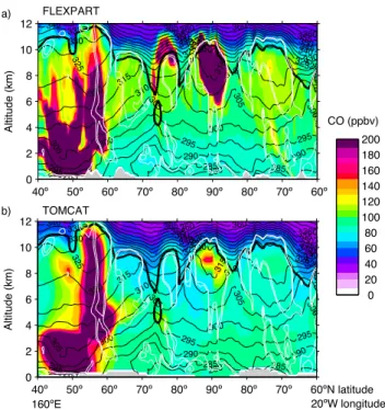
Figure 3 shows a vertical cross-section through the pollu-tion plume along 160◦E/20◦W across the pole as indicated in Fig. 2e, f. In the FLEXPART simulation (Fig. 3a) the mid-latitude plume is shown as a marked feature with high CO mixing ratios (>200 ppbv) over the pole directly below the tropopause. Isentropically, the air mass still carries a signa-ture of its origin near 40–50◦N with potential temperatures
of ∼320 K. In the TOMCAT simulation (Fig. 3b) the feature is more confined in the vertical and has lower mixing ratios (140–160 ppbv). Since CO mixing ratios are equally high in the area of the forest fire emissions near 50◦N, the difference between the two simulations is probably related to the differ-ent diffusion properties in the Lagrangian and the Eulerian model.
In addition, chemical loss and production processes in TOMCAT may also create some of the difference. In par-ticular oxidation with the hydroxyl radical (OH) is an im-portant, seasonally varying sink of CO in the atmosphere. During polar summer, model estimates of OH concentra-tions are about 10 times higher than during polar night (10– 15×105molecules cm−3 vs. <1×10⁵molecules cm−3, Bey
et al. (2001)). Simulated OH concentrations in CTMs are however uncertain (Shindell et al., 2008). Typical global at-mospheric lifetimes of CO against oxidation by OH are es-timated to about 2 months (Fisher et al., 2010). For Arctic summer conditions we assume shorter lifetimes, on the order of 2–4 weeks. It may be possible that the enhanced numer-ical diffusion of CO in the coarse-grid model also increases the effectiveness of the reaction with OH, which then would further contribute to lower CO concentrations. Unlike the
40°E 70°N 80°N 40°W 140°E 140°W a) b) 2 July 200 8 06 U TC 3 July 200 8 00 UTC 4 Jul y 2 008 00 UTC 5 Jul y 2 008 12 UTC c) d) e) f) g) h) FLEXPART TOMCAT 600 700 800 900 1000 1100 1200 1300 1400 1500 1600 mg m -2
Fig. 2. Total column CO (shading, mg m−2) during the period 2 July 2008 06:00 UTC to 5 July 2008 12:00 UTC in the FLEXPART model simulation (left column) and the TOMCAT model simulation (right column). The meteorological situation is denoted by the dynamic tropopause in the left column (2 pvu isoline at the 320 K isentrope, blue line) and sea-level pressure in the right column (white contours, 1010 to 970 hPa at 3 hPa interval) using ECMWF analysis data. Thick white line denotes the transect shown in Fig. 3.
280 285 285 285 290 290 290 295 295 295 300 300 300 305 305 305 30 5 310 310 0 1 3 315 315 315 320 320 320 325 325 325 330 330 330 335 335 340 340 340 345 345 350 350 355360 360 355360 365 Altitude ( km) 40º 160ºE 50º 60º 70º 80º 90º 80º 70º 60º 20ºW longitude 0 2 4 6 8 10 12 FLEXPART TOMCAT a) 0 20 40 60 80 100 120 140 160 180 200 CO (ppbv) 280 285 285 285 290 290 290 295 295 295 300 300 30 0 30 5 305 305 30 5 310 310 0 1 3 315 315 315 320 320 320 325 325 325 330 330 330 335 335 335 340 340 340 345 345 350 350 355360 360 355360 365 Alti tu de ( km) 40º 50º 60º 70º 80º 90º 80º 70º 60ºN latitude 0 2 4 6 8 10 12 b)
Fig. 3. Vertical cross-sections of CO concentrations in ppbv through
the Arctic atmosphere on 4 July 2008 00:00 UTC from 60◦N to
40◦N along 160◦E/20◦W through (a) the FLEXPART simulation
and (b) the TOMCAT simulation. Meteorological conditions are shown by contours of potential temperature (thin black lines), rel-ative humidity (80 and 90 percent, white solid lines), and the dy-namical tropopause (2 pvu, thick black line) from ECMWF analysis data.
TOMCAT model, the removal of CO by the reaction with OH is not represented in the FLEXPART model simulation. The combination of a fixed 20-day lifetime with the back-ground CO profile is intended to take this missing process to some extent into account implicitly.
3.1.2 Second episode, 6–10 July 2008
At the beginning of the second episode on 6 July 2008 06:00 UTC the large CO-rich plume over eastern Siberia in-trudes into the Arctic atmosphere, again ahead of a strato-spheric streamer (Fig. 4a). At the surface a low-pressure sys-tem is forming near 160◦E/70◦N (Fig. 4b). While the over-all size and shape of the plume agree very well between the two simulations, differences in the location and extent of the TCO maxima can be noted that are probably related to dif-ferent forest fire emission schemes and emission inventories (see Table 1).
On 7 July 2008 00:00 UTC (Fig. 4c, d), the polluted air-mass advances further towards the pole and the low-pressure system rapidly intensifies near the western tip of the advanc-ing mid-latitude airmass (170◦E/78◦N). The large plume elongates and reaches northern Greenland on 8 July 2008 12:00 UTC (Fig. 4e, f). The low-pressure system has
fur-ther deepened, reaching a minimum pressure of <986 hPa. The plume has acquired undulations along its outer boundary which are closely matched by the tropospheric wave guide (Fig. 4e, blue contour). The plume structure is quite similar in both models, but more diffusion of CO into the surround-ing air masses is apparent in the TOMCAT simulation. This agrees with the finding of Rastigejev et al. (2010) that a more complex plume boundary leads to its more rapid diffusive disintegration in Eulerian model simulations.
As on 10 July 2008 06:00 UTC the low-pressure sys-tem reaches Svalbard, it has heavily deformed the pollution plume, leading to its disintegration into separated maxima (Fig. 4h). Interestingly, the core of the low-pressure system itself appears to remain mostly free from mid-latitude pollu-tion. As the plume is split into smaller segments, the stronger diffusion in the Eulerian simulation rapidly smoothes the horizontal TCO structures. Evidently, the width of the plume in relation to the grid resolution influences how prone it is to numerical diffusion.
A vertical cross-section on 8 July 2008 12:00 UTC (Fig. 5) along 170◦W/10◦E as indicated in Fig. 4e, f shows the pro-gression of the polluted air mass towards the pole. The warm mid-latitude air masses have lifted the polar tropopause sub-stantially. As indicated by the white contours, the air mass is humid and mostly embedded in clouds. At about 78◦N the plume slides on top of the cold polar dome. Its lower boundary reaches to 5–6 km near the North Pole. The CO mixing ratios in FLEXPART are in general higher than in the TOMCAT simulation (Fig. 5a). This is particularly ev-ident close to the mid-latitude source regions, which would point to differences in the emissions, but in fact TOMCAT emissions are slightly higher than FLEXPART for biomass burning (Table 1). Hence, most likely, differences can be attributed to the reaction of CO with OH which is not rep-resented in the FLEXPART model. The diabatic transport processes that were involved in lifting this air mass near the polar tropopause are investigated in detail in a study based on aircraft data from the same campaign (Roiger et al., 2011).
3.1.3 Advection across the pole
The direct advection of the pollution plumes across the North Pole allows us to investigate effects of the numerical advec-tion scheme on the plume structure. Figure 6 shows a time sequence of the TCO field during 7 to 9 July 2008 as the pol-lution is crossing the pole. All data are shown directly on the output grid for clarity. While the TOMCAT model has to deal with the convergence of the meridians towards higher latitudes and a singularity at the pole, the Lagrangian FLEX-PART model is per design not prone to resolution issues, and in addition switches to a stereographic projection for calcu-lating advection in the vicinity of the pole.
On 7 July 2008 00:00 UTC, a small plume is shed east of the main plume that disperses quickly over the Russian Arc-tic (Fig. 6a, d, arrow). From the tropopause contour there
a) b) 6 July 200 8 06 U TC 7 July 200 8 00 UTC 8 Jul y 2 008 12 UTC 10 Jul y 2 008 06 U TC c) d) e) f) g) h) FLEXPART TOMCAT 40°E 70°N 80°N 40°W 140°E 140°W 600 700 800 900 1000 1100 1200 1300 1400 1500 1600 mg m -2
280 285 285290 290 295 295 295 300 300 300 305 305 305 310 310 310 315 315 32 0 320 320 325 325 325 33 0 330 330 335 335 335 340 340 345350 350345 350 355 355 355 360 365 Altitude ( km) 40º 50º 60º 70º 80º 90º 80º 70º 60º 0 2 4 6 8 10 12 280 285 285290 290 295 295 295 300 300 300 305 305 305 310 31 0 31 0 315 315 320 320 320 325 325 325 330 330 330 335 335 335 340 340 345350 350345 350 355 355 355 360 365 Alti tu de ( km) 40º 50º 60º 70º 80º 90º 80º 70º 60ºN latitude 0 2 4 6 8 10 12 170ºW 10ºE longitude FLEXPART TOMCAT a) 0 20 40 60 80 100 120 140 160 180 200 CO (ppbv) b)
Fig. 5. As Fig. 3, but for a vertical cross-sections through the Arctic
atmosphere on 8 July 2008 12:00 UTC from 60◦N to 40◦N along
170◦W/10◦E.
is no indication of a large-scale dynamic cause for this rapid spread. 12 h later, in the TOMCAT simulation another par-tial plume is circumnavigating the pole on the eastern side, associated with enhanced diffusion. This second feature is not visible in the FLEXPART simulation (Fig. 6b, e). Ap-parently, the minor plume is produced by the box grouping of the Prather et al. (1987) advection scheme in TOMCAT described earlier (Sect. 2.2). This results in a spreading of the tracer mass across a larger volume, and reduced CO mix-ing ratios. As the plume progresses further on 9 July 2008 00:00 UTC (Fig. 6c, f), the plume shape has regained some of the structure present before crossing the pole, effectively showing the result of the unpacking of second order moments from the Prather scheme. Given the difficulties of simulating a finely structured plume crossing the pole, and the relatively coarse grid resolution, the TOMCAT plume looks remark-ably similar to the FLEXPART simulation results at the end of the displayed time sequence.
To investigate the effect of horizontal grid resolution on the shape of the pollution plume, an additional model sim-ulation was conducted using the higher-resolution Eule-rian model WRF-Chem (Weather Research and Forecasting model coupled with Chemistry, Grell et al. (2005)). Re-sults from this simulation are not presented in detail here, see Sodemann et al. (2010) for a more extended discussion. The model was run for the period 25 June 2008 00:00 UTC 10 July 2008 18:00 UTC using 6-hourly 0.5◦×0.5◦ECMWF analysis as input data. The model domain covered the area
north of 20◦N at a horizontal grid resolution of 50 km, with
34 vertical levels up to 20 hPa. WRF-Chem simulates the shape of the pollution plume during passage over the North Pole as an intermediary between the FLEXPART and TOM-CAT simulations. Numerical diffusion was clearly leading to smoother gradients than the Lagrangian FLEXPART simula-tion, albeit some more fine-scale structure could be retained than in the coarse-grid Eulerian TOMCAT simulation (see Sodemann et al. (2010), Fig. 6).
3.2 Comparison with satellite observations
The comparison between the two transport models FLEX-PART and TOMCAT has shown that the structures of the CO-rich air masses are overall similar in shape, in particular for larger features. Smaller features and finer-scale structures however are represented quite differently in their concentra-tion gradients. Satellite remote-sensing data are employed now to compare both model simulations in terms of spatial structure and magnitude of TCO to a reference data set.
Figure 7 shows daily composites of all daylight retrievals of the satellite observations and the model fields sampled at the same space/time locations during 3–8 July 2008. Due to the daily compositing, the structures in Fig. 7 do not find their direct correspondence in the time snapshots of TCO dis-played in Figs. 2 and 4. The gray area in the IASI observa-tions (Fig. 7, center column) are missing data due to impen-etrable cloud cover. Most thick clouds are in mid-latitudes and over forest fires as in Canada, while the view into the Arctic atmosphere is mostly cloud-free. The low values over Greenland in all panels are due to the reduced atmospheric column over orography (Pommier et al., 2010). Both models were weighted with local daily mean IASI averaging kernels (see Sect. 2).
On 3 July 2008 (Fig. 7a–c), both models and the satellite image show the first, smaller plume between eastern Siberia and the North Pole as a hook-like structure. The TCO maxi-mum over south-eastern Siberia, over Scandinavia and south of Greenland are other areas with good model/satellite cor-respondence. Agreement is less good over western North America and Alaska. Maximum values in the IASI data are beyond the color scale (>1700 mg m−2). Visually, the IASI TCO observations appear more similar to the FLEXPART model than to TOMCAT. On average, the median of the dif-ference between IASI and FLEXPART TCO is 53 mg m−2, while the TOMCAT TCO is 188 mg m−2 lower than IASI (note the different color scale in Fig. 7, right column). Throughout the simulation, CO concentrations are increas-ing in the FLEXPART simulation which leads to larger biases compared to IASI in the beginning (median 102.4 mg m−2on
2 July 2008) than in the end (0.5 mg m−2on 10 July 2008). On 4 July 2008 (Fig. 7d–f), IASI shows the curled-up plume with two clear TCO maxima near the pole. While the Lagrangian FLEXPART model represents the structure of the maxima well, it is beyond the resolution of the Eulerian
-2 mg m a) 7 July 2008 12 UTC FLEXPART TOMCAT
8 July 2008 00 UTC 9 July 2008 06 UTC
b) c) d) e) f) 600 800 1000 1200 1400 1600 40°W 40°E 140°E 140°W x80°N
Fig. 6. Zoomed view of total column CO (shading, mg m−2). (a–c) Total column CO from the FLEXPART simulation on 7 July 2008 12:00 UTC, 8 July 2008 00:00 UTC and 9 July 2008 06:00 UTC. (d–f) Total column CO from the TOMCAT simulation for the same period. White contour shows the dynamical tropopause at 320 K (2 pvu). Data are shown on the output grid without spatial interpolation.
TOMCAT model to realistically represent concentrations during this break-up. This is more obvious one day later on 5 July 2008 (Fig. 7g–i), where IASI and FLEXPART, but not TOMCAT, show a narrow, elongated feature reaching from the pole towards Scandinavia. The filament was ∼220– 300 km wide, at an elongation of ∼2500 km, both in the IASI data and the FLEXPART simulation. Another filament ex-tending towards the Canadian Arctic in the FLEXPART sim-ulation was only ∼100 km wide, but appears broader in the satellite observation. The finding that such a narrow filament both in extension and location is very closely simulated by FLEXPART is an impressive demonstration of the capabili-ties of a Lagrangian model.
As the large pollution plume is advancing towards the pole on 6 and 7 July 2008 (Fig. 7j–l and m–o), both models agree well with the IASI observation. At that time, the plume is between 850 km and 1600 km wide, indicating the scale of pollution features which is also well represented in the TOM-CAT model. The larger size of the polluted airmass leads to a smaller influence of numerical diffusion, and better corre-spondence between models and satellite retrievals. The TCO maxima in the large plume agree well between the models on 7 July 2008, also as it is reaching northern Greenland on 8 July 2008 (Fig. 7p–r). TCO concentrations at the eastern flank of the plume are lower, possibly due to differences in the biomass burning emission scheme.
In general, it is remarkable how well the structure of the pollution plumes agree between the satellite observations and both model simulations. This underlines that (i) the plumes simulated by the models have very similar correspondence in the real world as seen by the IASI satellite, and (ii) the
ECMWF analysis data that are used for driving both model simulations are very reliable, even at high latitudes where weather observations at the surface are generally sparse.
The better agreement between the IASI observations and the FLEXPART simulation in particular for fine-scale struc-tures leads to the conclusion that the sharp gradients and nar-row features predicted by the Lagrangian model (Sect. 3.1) are indeed a real feature of atmospheric transport at these high latitudes. Not surprisingly, the Eulerian model has too much numerical diffusion at the grid-resolution applied here, which leads to an unrealistic smoothing of the TCO gradi-ents, and the disappearance of fine-scale features.
It is interesting to compare the TCO fields from the model simulations and the IASI satellite quantitatively. Figure 8a, b show the probability density distributions of a correlation be-tween all IASI observations and the FLEXPART and TOM-CAT model simulation, each transformed with the respective IASI AK. FLEXPART deviates from the IASI observations, with the exception of values at ∼800 mg m−2TCO, which is the level of background concentrations. FLEXPART data be-low ∼650 mg m−2TCO are typically lower due to the under-lying orography, with increasing concentrations scatter also increases. For values above ∼1500 mg m−2 TCO, part of
the AK-weighted FLEXPART data show a high bias. The comparison between IASI and the TOMCAT data (Fig. 8b) shows a clear low bias that becomes stronger for values above
∼800 mg m−2TCO. The reason for the lower TCO values in TOMCAT compared to Figs. 2, 4 is that applying the IASI averaging kernels emphasizes the upper-tropospheric part of the atmospheric column (Fig. 1a), where TOMCAT has the strongest low bias (Fig. 1b). Additionally, there is a cloud
c) b) a) 140°W CAT 140°E 40°W 40°E 70°N 60°N 80°N M O T IASI FLEXPART 3 July 2008 4 July 2008 5 July 2008 6 July 2008 7 July 2008 8 July 2008 f) e) d) i) h) g) l) k) j) o) n) ) m r) q) p) 60 0 70 0 800 900 1000 11 00 12 0 0 13 0 0 14 0 0 15 0 0 16 0 0 mg m-2 700 800 900 1000 1100 12 00 1300 1400 1500 1600 1700 70 0 80 0 900 1000 1100 12 00 13 0 0 14 0 0 15 0 0 16 0 0 17 0 0
Fig. 7. Comparison of total column CO from FLEXPART (left column), IASI (center column) and TOMCAT (right column) in mg m−2 during 3 to 8 July 2008. Displayed are IASI daylight composites. Model data are interpolated to the same time and location as the satellite retrievals and weighted with a mean IASI averaging kernel. Cloudy pixels in the IASI data are shown in white as missing data.
IASI TOC CO (mg/m2) FLEXPART AK TOC CO (mg/ m 2) 0 500 1000 1500 2000 2500 3000 0 500 1000 1500 2000 2500 3000 IASI TOC CO (mg/m2) TOMCAT AK TOC CO (mg/ m 2) 0 500 1000 1500 2000 2500 3000 0 500 1000 1500 2000 2500 3000 FLEXPART no AK TOC CO (mg/m2) FLEXPART AK TOC CO (mg/ m 2) 0 500 1000 1500 2000 2500 3000 0 500 1000 1500 2000 2500 3000 a) b) c)
Fig. 8. (a) Probability density distribution of AK weighted FLEXPART simulation vs. IASI retrievals, (b) AK weighted TOMCAT simulation vs. IASI retrievals, (c) AK weighted FLEXPART simulation vs. FLEXPART simulation without AK weighting. Contour intervals are
(1,2,5) × 10−4,(1,2,5) × 10−3,(1,2,5) × 10−2,1 × 10⁻¹.
of data points of IASI TCO above 2000 mg m−2 that cor-responds to data points of TOMCAT TCO of only about 700 mg m−2. These data points are mostly located in the first, narrow CO plume that is removed too quickly by numerical diffusion in the TOMCAT model. Further possible causes of low biases of the model simulations are further investigated in Sect. 4.
In this context it is insightful to investigate how the ac-tual model TCO values compare with the simulated retrieval values. Figure 8c compares the TCO data points from the FLEXPART simulation without application of an AK vs. such weighted with the mean IASI AK (Eq. 1). The sim-ulated retrievals are much higher than the model data with-out kernel weighting. The overestimation increases steeply, despite some scatter, with increasing CO concentrations for values larger than ∼800 mg m−2TCO. Effectively, the simu-lated retrieval has more pronounced maxima than the model atmosphere actually contains. This can be seen by comparing e.g. Figs. 2a and 7a. One possibility is that the background added to FLEXPART may be too high in the upper tropo-sphere, while the prior is higher in the lower troposphere than the mean of the observations (Fig. 1b). In combination, the application of an AK then stretches the range of values to ex-cessively high values compared to the simulated state of the atmosphere. This kind of diagnostic could be useful to test the influence of an a priori that varies with latitude and sea-son on simulated retrievals. One implication may be that the IASI data used here overestimate the pollution of the upper troposphere, and actually represent an atmosphere closer to the state represented in the FLEXPART model.
3.3 Comparison between models and CALIPSO data
The vertical distribution in the atmosphere is an important factor determining the lifetime and transport of CO released from forest fires. The vertical location of CO in the model simulations is first determined by the emission schemes em-ployed by the models. During atmospheric transport, lift-ing approximately along isentropes or fronts and mixlift-ing take place. While the horizontal structure of pollution plumes can
Altitude (km) 2 0 4 6 8 10 12 0 2 4 6 8 10 x 10−3 0 0.05 0.1 0 2 4 6 8 10 12
AttCol, AttDep (AU)
AttCol AttDep 280 280 285 285 290 290 290 295 295 295 300 300 300 305 305 305 310 310 31 0 315 315 315 320 320 320 325330 325 325 330 330 335 335 335 340 340 340 345 345 345 350 355 350 350 355 355 360 360 Altitude (km) 0 2 4 6 8 10 12 0 5 10 15 20 280 280 285 285 290 290 290 295 295 295 300 300 300 305 305 305 310 310 31 0 315 315 315 320 320 320 325330 325 325 330 330 335 335 335 340 340 340 345 345 345 350 355 350 350 355 355 360 360 Latitude/Longitude (º) Altitude (km) 80.1/ 43.2 81.3/ 28.5 81.8/ 10.8 81.5/ −7.3 0 2 4 6 8 10 12 0 50 100 150 200 a) b) c) d)
CALIOP attenuated backscatter @ 532nm
FLEXPART CO (ppbv)
FLEXPART BC (pptv)
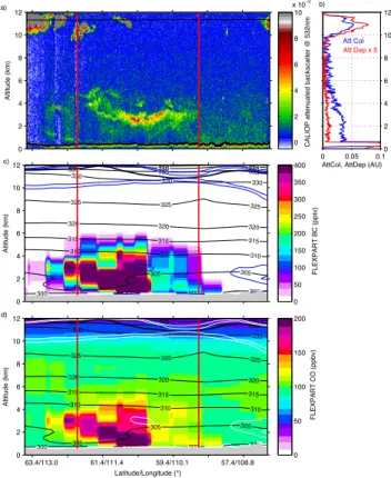
Fig. 9. Comparison of simulation data with the space-borne CALIPSO lidar for an aerosol feature observed on 5 July 2008 07:00 UTC near Greenland (see Fig. 2d). (a) Aerosol backscatter and depolarization from the CALIPSO satellite and vertical mean for the feature delineated by red vertical lines, (b) Mean profiles of attenuated color ratio (blue, AttCol) and attenuated depolariza-tion (red, AttDep) in arbitrary units averaged over the segment marked by red lines in panel (a), (c) FLEXPART black carbon tracer concentration (pptv), (d) CO concentration (ppbv) from FLEX-PART. Meteorological conditions are indicated by the dynamical tropopause (2 pvu, thick black and white contour), potential tem-perature (thin black contours), and relative humidity (80% and 90%, blue and white contours) from ECMWF analyses. Red lines indi-cate the location of the aerosol feature.
be readily measured from satellite platforms, it is consider-ably more challenging to validate the vertical structure of the transport model simulations. Here we use the aerosol mea-surements from the space-born lidar instrument CALIOP as a proxy for pollution transport in the models. As we do not simulate aerosols in the TOMCAT model this comparison is carried out using the FLEXPART model only.
Out of 10 opportunities during the study period where aerosol was clearly detected in the CALIPSO profiles two cases have been selected where aerosol was at high and medium-low altitudes, respectively. A first case has been identified where aerosol is visible in the highly lifted and filamented plume that is exiting the Arctic on 5 July 2008 07:09 UTC near 20◦E/81◦N (compare Fig. 2g, h). An area of enhanced color ratio and with low attenuated depolariza-tion is visible at altitudes of 10–12 km in the secdepolariza-tion of the curtain contained by the red markers (Fig. 9b). The much stronger backscatter signal further to the right in Fig. 9a in-dicates an ice cloud.
The discrimination between clouds and aerosols in CALIOP observations is performed based on the differences in their optical and physical properties. It is based on an au-tomated cloud and aerosol discrimination (CAD) algorithm (Liu et al., 2009). The CAD algorithm is a multidimensional, at present latitude-independent, probability density function (PDF) based approach (Liu et al., 2004). Attributes used are lidar backscatter intensity, wavelength dependency, depolar-ization ratio, layer heights or ancillary parameters (e.g., tem-perature, pressure, location, season). The algorithm is most representative of the cloud and aerosol distributions at lower latitudes. Therefore, some misclassifications of optically thin polar clouds (or edges of such clouds) can occasionally oc-cur.
Low depolarization indicates spherical particles and a con-stant color ratio confirms a uniform particle size is seen in the volume over the section of the curtain contained by red markers (Fig. 9b). Nevertheless, this feature is classified as cloud, partly with low or no confidence, and as stratospheric feature, by the CALIPSO CAD (not shown).
The cross-section through the black carbon tracer field of the FLEXPART model (Fig. 9a) shows a maximum at the same altitude but slightly displaced horizontally. The ECMWF tropopause (thick black contour) is somewhat ele-vated at this location, probably due to diabatic effects as indi-cated by the high relative humidity (blue contours). Note that the BC tracer apparently has partly been lifted into the strato-sphere. The FLEXPART CO tracer shows that the aerosol in the tropopause region is a remainder of a deeper and more extensive pollution feature (Fig. 9c). Several subsequent CALIPSO crossings at later times confirm the observation of this elevated aerosol plume (not shown). The good co-location of these observations with the FLEXPART black carbon tracer, strengthens the indication that the CALIOP feature is indeed aerosol, wrongly classified as cloud struc-ture.
A second case is a crossing of the CALIPSO satellite over a large active forest fire in Siberia near 110◦E, 60◦N on 8
July 2008 19:22 UTC (Fig. 4e, f). The CALIPSO curtain shows the aerosol load as high attenuated backscatter with a maximum at ∼3 km altitude, and extending to above 5 km in the vertical (Fig. 10b).
The mean profiles of attenuated depolarization and color ratio confirm the presence of aerosol more clearly than in the previous case. The CALIPSO vertical feature mask identifies the region clearly as aerosol (not shown). In the FLEXPART BC tracer field, a strong aerosol signal can be seen that cor-responds well with the horizontal location of the feature in the CALIPSO data. The feature however has a distinctively lower vertical extent in the simulation (Fig. 10a, c). The max-imum of the BC tracer is located near the surface instead of at higher altitudes, and the aerosol does not reach as high as observed. This is probably due to the forest fire emis-sion scheme in FLEXPART, which places the smoke plume directly in the lowest 0–150 m above ground and relies on turbulent transport and mixing processes to distribute the CO tracer in the vertical. This procedure likely concentrates the CO and aerosol near ground level.
In summary, the validation of the horizontal structure of the model simulations provides independent validation of the simulated forest fire plumes. While the vertical altitude of one feature is well simulated, some deficiencies in the verti-cal distribution of aerosol tracer near the emission source in FLEXPART are identified.
3.4 Comparison between models and in situ aircraft
data
In-situ CO observations of the NASA aircraft DC-8 during flight 22 on 9 July 2008 allow us to evaluate the validity of the model simulations against an independent data set of in-situ observations. The flight data provides local information about the small-scale structure of pollution plumes, the lay-ering, and the strength of gradients. For the comparison, CO mixing ratios along the flight track have been extracted from the FLEXPART and TOMCAT simulations.
The aircraft flew first over Greenland towards the south for an inter-comparison with the DLR Falcon, then north up to 88◦N, and back to Thule airport (Fig. 11a). Along the way, the aircraft made several profiles to probe the vertical extent of pollution layers (Fig. 11b). During the first leg of the flight, the aircraft encountered moderately polluted layers of around 100–150 ppbv CO mostly at altitudes between 6– 8 km (Fig. 11c, red line). While both models follow the gen-eral trend of the aircraft data, both underestimate the variabil-ity. A low bias is visible in the TOMCAT data, which appears consistent with the lower background concentrations already identified in Fig. 1b. FLEXPART’s tagged tracers indicate that the pollution enhancement at higher altitudes originates from biomass burning, as can be seen from the offset of the solid black line over the gray shaded area.
Altitude (km) 0 2 4 6 8 10 12 a) b) c) d) 0 2 4 6 8 10 x 10−3 0 0.05 0.1 0 2 4 6 8 10 12
AttCol, AttDep (AU)
Att Col Att Dep x 5 300 305 300 300 300 305 305 310 310 310 315 315 315 320 320 320 325 325 325 330 330 330 335 335 335 340 340 340 345 345 350 345 Altitude (km) 0 2 4 6 8 10 12 0 50 100 150 200 250 300 350
CALIOP attenuated backscatter @ 532nm
FLEXPART CO (ppbv) FLEXPART BC (pptv) 400 300 305 300 300 300 305 305 310 310 310 315 315 315 320 320 320 325 325 325 330 330 330 335 335 335 340 340 340 345 345 350 345 Altitude (km) 0 2 4 6 8 10 12 0 50 100 150 200 57.4/108. 61.4/111. 59.4/110. Latitude/Longitude (°) 63.4/113.0 4 1 8
Fig. 10. As Fig. 9, but for an aerosol feature observed on 8 July 2008 19:00 UTC (see Fig. 4c).
As the aircraft is heading north at 15:00 UTC it enters stratospheric air with low CO concentrations. At around 15:45 UTC it abruptly enters an airmass with significantly enhanced pollution levels, reaching up to 240 ppbv CO at around 8 km altitude (Fig. 11c). During this part of the flight, both models show very good agreement with the flight data. Drops in pollution levels during downward and upward pro-files in the observations and model data indicate that the ver-tical structure of the pollution is well represented. Some of the CO enhancement observed by the aircraft originates from biomass burning as identified by FLEXPART’s tagged trac-ers (gray area).
For further comparison, a backward analysis of the DC-8 flight was performed using FLEXPART. For the series of backward simulations along the flight track, the model is initialized in a very small volume around every flight po-sition, whereas the forward simulation output is sampled along the flight track at the relatively coarse 0.5◦ grid
res-olution. Thus, a backward simulation takes full advantage of the Lagrangian nature of the model and allows even finer-scale structures to be resolved than with the forward simu-lation, as shown by Stohl et al. (2003). A large number of air parcels (60 000) were tracked backwards from locations along the flight track of the aircraft when its position had changed more than 0183◦ horizontally or 100 m vertically.
Emissions in the surface layer were then integrated along the trajectories of the air parcel to construct estimates of CO con-centration. Figure 11d compares this backward product for biomass burning emissions and combined anthropogenic and biomass burning emissions to the DC8 CO measurements. It can be seen that a number of the peaks in the observational time series are better matched in the backward product (e.g. near 16:20 UTC or 17:40 UTC) which are due to forest fires. Also, more fine-scale structure is present in the model time series. In a few cases, the backward product is worse than the forward product (e.g. near 14:50 UTC). At 75◦latitude and typical airspeed of the DC-8, the backward run FLEX-PART data resolves features of about 10–30 km width. The 10 s averaged CO data from the DC-8 can resolve features of up to 2.5 km length. Thus, even with a perfectly simulated advection of the plume, FLEXPART would miss some of the variability measured by the aircraft.
The vertical structure of the pollution is further investi-gated by a comparison between the vertical CO curtains from both models along the flight track, and the DIAL aerosol li-dar onboard the NASA DC-8 (Fig. 12a). While the aerosol backscatter lidar signal is not directly comparable to the CO field in the model simulations, it gives some indication of vertical and horizontal positioning of pollution plumes, and the location of maxima. As can be seen most clearly in the TOMCAT and FLEXPART CO mixing ratio curtains (Fig. 12c,e), the aircraft probed two major pollution areas, a first one that is of smaller scale and at altitudes between 6– 10 km, on the southern part of the flight track over Greenland (Fig. 11a). Later on a second, broader plume of higher CO concentrations was reached north of Greenland that also ex-tends over a larger range of altitudes (4.5–11 km), and was located over the Canadian Arctic (Fig. 11a).
While the location of the maximum of the first feature in terms of altitude and extent agrees well between FLEXPART and the DC-8 lidar data, the maximum is more diffuse and has a larger horizontal extent in the TOMCAT simulation. As indicated by the relative humidity data from ECMWF (Fig. 12b, blue contours) at least some of the backscatter in the aerosol plot likely originates from clouds. The dynamical tropopause from the ECMWF analysis (thick red line) con-firms that the aircraft was located within the stratosphere at around 15:30 UTC.
The second feature, which is delimited towards the south by ice clouds (dark red area in Fig. 12a) is simulated quite differently in terms of CO structure by the two mod-els. While FLEXPART distributes the CO pollution roughly co-located with the clouds and down to altitudes of 3 km (Fig. 12c), in TOMCAT the pollution plume has a core of high values at about 7 km altitude. As Fig. 11c demon-strates, both shapes of the plume provide a more or less real-istic simulated CO measurement along the DC-8 flight, even though TOMCAT has a low bias at around 17:00 UTC. Ver-tical transport in the two models appears to have brought the biomass burning emissions into different atmospheric
12:00 13:00 14:00 15:00 16:00 17:00 18:00 0 2 4 6 8 10 b) c) d) Altitude ( km) 65 70 75 80 85 90 Lat itud e ( N ) Alt 12:00 13:00 14:00 15:00 16:00 17:00 18:00 50 100 150 200 250 CO ( pp bv) DC8 TOMCAT FLEXPART forward BB FLEXPART forward AN+BB
12:00 13:00 14:00 15:00 16:00 17:00 18:00 50 100 150 200 250 Time (UTC) CO (pp bv) DC8 FLEXPART backward BB FLEXPART backward AN+BB Lat 700 800 900 1000 1100 1200 1300 1400 1500 1600 1700 a) mg m -2
Fig. 11. Flight 22 on 9 July 2008 of the NASA DC-8. (a) Flight track (black line) overlaid on FLEXPART total column CO (mg m−2) on 9 July 2008 15:00 UTC. Orography has been filled with background CO concentrations to make the plume uniformly visible. (b) Flight altitude from Global Positioning System data (solid line) and latitude (dashed line). (c) CO measurements from the DC-8 (red) compared to FLEXPART biomass burning CO (gray shading), FLEXPART anthropogenic CO (black solid line) and TOMCAT model data (blue line) interpolated to the location of the aircraft in ppbv. (d) CO measurements from the DC-8 (red) compared with backward products of the FLEXPART model for biomass burning CO (gray shading) and combined anthropogenic and biomass burning CO (black line) in ppbv.
layers, and thus the core of the polluted air reaches fur-ther down in the FLEXPART simulation (Fig. 12c). Possi-bly, part of the difference is related to the fact that FLEX-PART treats agricultural and wildfires differently, whereas in TOMCAT the emissions are distributed evenly over a day starting at 00:00 UTC. Unfortunately this region was not di-rectly probed by the aircraft. However, the DIAL data and FLEXPART aerosol tracer show a similar upper boundary at
∼17:00 UTC (Fig. 12a, b).
The black carbon tracer from FLEXPART indicates the presence of some aerosol in both major plumes (Fig. 12b). While in the first plume the aerosol is near the tropopause, the second plume has a simulated aerosol maximum at lower levels. The cloudiness of the scene makes a comparison to the DIAL data difficult. Some of the finer aerosol lay-ers at intermediate levels 6–8 km that are apparent in the DIAL data between 12:00–16:00 UTC are not simulated by FLEXPART. A separation of the CO enhancement in FLEX-PART due to forest fires (Fig. 12d) and Asian anthropogenic emissions (Fig. 12f) highlights that the pollution is vertically stacked, similar to the aerosol mixing ratios: the first plume contains mostly forest fire emissions, while the second plume is of Asian fossil fuel combustion origin above about 6–7 km altitude and of mixed Siberian forest fire and Asian fossil
fuel combustion origin below. Thus, during advection the airmass had incorporated other polluted air masses of East Asian (Chinese) origin (Roiger et al., 2011).
4 Discussion
4.1 Transport with Arctic low-pressure systems
The pollution transport across the North Pole in association with low-pressure systems as shown here suggests that this could be an effective transport mechanism for polluted mid-latitude air to the Arctic atmosphere. While it may appear rare to observe two low-pressure systems in the proximity of the North Pole within such a short time period, it is well established that the mean SLP field during northern hemi-sphere (NH) summer (JJA) has a SLP minimum near 85◦N,
180◦E (Reed and Kunkel, 1960; Serreze and Barrett, 2008).
Tracking cyclones in the NCEP (National Center for Envi-ronmental Prediction) reanalysis data for the period 1971– 2000, Orsolini and Sorteberg (2009) found that the Arctic SLP minimum is established by about 20 cyclonic systems each season that slow down and finally decay near the central Arctic ocean. Most of these systems originate in a baroclinic zone located along the Eurasian coast that presumably is