EvoEvo Deliverable 2.7: Specifications of the integrated evolutionary model

HAL Id: hal-01577147

https://hal.archives-ouvertes.fr/hal-01577147

HAL is a multi-disciplinary open access archive for the deposit and dissemination of sci-entific research documents, whether they are pub-lished or not. The documents may come from teaching and research institutions in France or abroad, or from public or private research centers.

L’archive ouverte pluridisciplinaire HAL, est destinée au dépôt et à la diffusion de documents scientifiques de niveau recherche, publiés ou non, émanant des établissements d’enseignement et de recherche français ou étrangers, des laboratoires publics ou privés.

To cite this version:

Guillaume Beslon, Charles Rocabert. EvoEvo Deliverable 2.7: Specifications of the integrated evolu-tionary model. [Research Report] INRIA Grenoble - Rhône-Alpes. 2015. �hal-01577147�

Page 1 of 22

EvoEvo Deliverable 2.7

Specifications of the integrated evolutionary

model

Due date: M12 (November 2014)

Person in charge: Guillaume Beslon Partner in charge: INRIA

Workpackage: WP2 (Development of an integrated modeling platform)

Deliverable description: Specificiations of the integrated evolutionary model: Description of the modeling choices for the integrated model. This model should include most of the choices made for deliverables D2.2, D2.4 and D.2.6.

Revisions:

Revision no. Revision description Date Person in charge

1.0 First version of the integrated evolutionary model 22/11/14 C. Rocabert (INRIA) 1.1 Corrections and additions by G. Beslon and C. Rocabert 29/11/14 C. Rocabert (INRIA) 1.2 Finalized version, transmitted to the partners 03/02/15 C. Rocabert (INRIA)

Page 2 of 22

Table of Contents

1.

2.

2.2.

2.3.

3.

3.1.

3.2.

4.

4.1.

4.2.

5.

5.1.

5.2.

6.

7.

7.1.

7.2.

8.

9.

Page 3 of 22

1. Introduction

The development of an integrated evolutionary model including multiple levels of selection is the ultimate goal of the Work Package 2 (WP2). As described in WP2 objectives, submodels produced in deliverables 2.1, 2.3 and 2.5 can be exploited separately (and this idea has been fully applied since an independent release exists for each model), but they are designed to be part of a nested model.

Two major objectives constrained the development of the integrated model:

1) Integrate all the biological levels (genome, metabolic network, population…) we consider to be mandatory to explore deeply Evolution of Evolution. The realism of each level is an essential element to observe complex enough genotype-to-phenotype mapping and fitness landscape,

2) Maintain the model complexity low enough to enable its practical use.

Clearly both objectives are antagonistic and their balancing has often driven the modeling choices described in this document.

The integrated model is rooted in the knowhow of the EvoEvo partners, mainly INRIA and University of Utrecht (UU) and more generally in the field of Evolutionary Systems Biology (ESB, see Soyer & O’Malley, 2013). Such a disciplinary background implies some choices in the way biological processes are represented and the genotype-to-phenotype mapping takes a central place in that matter. Indeed, evolution shapes it, leading to diverse outcomes such that robustness, evolvability, or open-endedness. Another essential concept is the fitness landscape, which gives a direction to evolution, and defines the selective pressures. The concept of genotype-to-phenotype mapping naturally leads to the concept of levels (at least the genotype and the phenotype). The phenotype is encoded in the genotype, and is instantiated through the genotype-to-phenotype mapping. In the ESB field, a distinction is usually made within an organism between “levels” depending on the scale and the nature of implied biomolecules, e.g. the genome (made of DNA), the transcriptome (RNA molecules), the proteome (proteins) or the metabolome (metabolites and small components), but also higher levels such that tissues, organs, population, and so on. Those levels are considered as highly complex dynamic systems owing to the large number of interactions, layered in several networks (e.g. the genetic regulation network, the protein-protein network, the metabolic network, the trophic network…).

The EvoEvo project aims at studying bacterial evolution (Hindré et al., 2012). INRIA and UU have developed independently two formalisms that are specifically dedicated to the study of indirect selection in unicellular populations. INRIA used the “sequence-of-nucleotides” formalism to develop the aevol model (Knibbe et al., 2007a; Knibbe et al., 2007b). Using this formalism, INRIA showed that indirect selection could select specific genetic and transcriptomic structures depending on the mutational and selective pressures (Knibbe et al., 2007b; Beslon et al., 2010a; Beslon et al., 2010b). UU proposed the “pearls-on-a-string” formalism and showed that in time varying environments regulation networks, metabolic networks and species networks can acquire structures that increase the evolvability of organisms (see for example Crombach & Hogeweg, 2008; Cuypers & Hogeweg, 2012). However, both formalisms are restricted to specific levels of organization. In the integrated model, we push the model complexity one step further, by including in one single model a genome structure, a genetic regulation network (GRN), a metabolic network,

Page 4 of 22 a population and its environment. In practice, the model explicitly includes all those levels as predefined interacting classes. Higher levels of selection may emerge through evolution, such that trophic networks, ecosystems, and so on.

Each level of selection and its interactions will be described in this deliverable. Section 2 presents the modeling choices made on the genotype-to-phenotype mapping and on the artificial chemistry. Sections 3, 4 and 5 deal with the genome structure, the genetic regulation network, and the metabolic network. Then, section 6 introduces the population level, and the interactions it allows between individuals and their environment.

2. Genotype-to-phenotype mapping and artificial chemistry

2.1. Reminder: the

𝒏-tuple bag as a common formalism

A 𝑛-tuple is an ordered list 𝑥!, 𝑥!, … , 𝑥! :  𝑇!  ×  𝑇!  ×  …  ×  𝑇! with 𝑇 the “product type” of 𝑥! (e.g. ℝ, ℕ, …). In both the “sequence-of-nucleotides” and “pearl-on-a-string” formalisms, the genotype-to-phenotype mapping is based on the extraction of an unordered set of 𝑛-tuples from the genotype (a “bag” of 𝑛-tuples1_{). Specified operators project the genome on a 𝑛-dimensional space (figure 1).}

The bag of 𝑛-tuples is then used to build the higher organism level in another specified space (a fuzzy set in aevol, or a GRN in pearls-on-a-string models). For example, aevol uses a complex and non-linear artificial genetic code to extract a set of triplets 𝑥!, 𝑥!, 𝑥! ∶   ℝ! from a circular double strand binary sequence. The mapping is done in two steps: the transcription and the translation. In “pearls-on-a-string” models, the genome is directly encoded as an ordered set of 𝑛-tuples. Depending on the complexity of projection operators, evolution outcomes on the genome structure and the mapping will not be the same. In both models, the locus of the 𝑛-tuples set do not impair fitness, but, since the 𝑛-tuples are encoded locally in the genome (in coding regions, or in pearls), the modification of their position (and relative positions) on the sequence can affect the organism’s evolution on the long term.

Figure 1 - A set of 𝑛-tuples is extracted from the genome data-structure by projecting it on a 𝑛-dimensional space with specified operators. This projection can be a simple translation or a complex non-linear process (a mapping).

1

This idea is directly inspired from the – simplistic – description of the cell as a “bag-of-proteins”.

Genome space

n-tuples n-dimensional space Projection or Mapping

Page 5 of 22

2.2. Basic concepts on artificial chemistries

An artificial chemistry (AChem) can be defined as a triplet (𝑆, 𝑅, 𝐴), where 𝑆 is the set of all possible molecules, 𝑅 is a set of reaction rules representing the interactions among the molecules, and 𝐴 is an algorithm describing the reaction vessel or domain and how the rules are applied to the molecules inside the vessel (Dittrich et al., 2001).

The set of molecules 𝑆   =   {𝑠_!, 𝑠_!, . . . , 𝑠_!} can potentially be infinite. A reaction rule 𝑟   ∈  𝑅 is a chemical equation 𝑠!   +   𝑠!  +  . . . +  𝑠!   →   𝑠!!   +   𝑠!!  +  . . . +  𝑠!!, with the reactants (or the substrates) on the left side and the products on the right side, 𝑖 being the order of the reaction. The set of reaction rules 𝑅 can be defined explicitly (all possible reactions 𝑟 are defined and are in finite number), or implicitly. In this example, stoichiometry is 1 for all reactants, but there is no constraint on this point. The algorithm 𝐴 is applied on an instance of 𝑆, that is, a collection 𝑃 of molecules. The set of chemical equations 𝑅 can be solved with stochastic or deterministic methods, possibly adding spatial rules.

2.3. Defining an artificial chemistry with the

𝒏-tuples bag formalism

We distinguish two ways to define an artificial chemistry with a 𝑛-tuples bag:

(1) Each 𝑛-tuple codes for a reaction rule. In this case, each organism owns a specific set of reactions rules 𝑅, somehow carrying its own artificial chemistry. For instance, a 𝑛-tuple

𝑥!, 𝑥!, … , 𝑥!, 𝑥!!!, 𝑥!!!, … , 𝑥! could define the chemical equation of order 𝑛/2: 𝑠!   +   𝑠!   +   …  +   𝑠!

!   →   𝑠!!!!+   𝑠!!!!+ ⋯ +   𝑠! with 𝑥_!≡ 𝑠_!, 𝑖   ∈   {0,1,2, . . . , 𝑛}.

Additional elements in the tuple can be used to define the reaction rates and the stoichiometry. (2) Each 𝑛-tuple codes for a chemical species, being potentially a reactant for a subset of reactions in 𝑅. In this case, 𝑅 is defined once for all the cells, a reaction occurring only if all the reactants are present in the cell. For instance, let’s consider the set of reaction rules 𝑅 containing reactions (1) 𝑠_!+ 𝑠_!⟷ 𝑠_!. 𝑠_! and (2) 𝑠_!. 𝑠_! → 𝑠_!+   𝑠_! (𝑠_!, 𝑠_!, 𝑠_! ∈ 𝑆, and "." representing a chemical bond), the singleton (𝑥_!), with 𝑥_!≡ 𝑠_!,  catalyses the enzymatic reaction 𝑠_!+ 𝑠_!⟷ 𝑠_!. 𝑠_! → 𝑠_!+   𝑠_!. A pair (𝑥_!, 𝑐_!) with 𝑐! the concentration of 𝑥!, could be used, and so forth. A 𝑛-tuple could also produce useless compounds, not being reactant of any reactions.

The 𝑛-tuple formalism actually gives us a general framework to develop an artificial chemistry (figure 3).

Page 6 of 22

Figure 2 - A general framework for the 𝑛-tuples bag formalism. (A) At each replication, the genome data-structure undergoes mutations (point mutations, large rearrangements, recombinations, horizontal transfers). (B) A mapping corresponding to the transcription and translation processes, gives a set of 𝑛-tuples. (C) Depending on modeling choices, the set of 𝑛-tuples defines: (i) an independent set of reactions rules 𝑅 in each cell, or (ii) chemical products (proteins, catalysts, metabolites...) involved or not in a subset of reactions belonging to a predefined set of reactions 𝑅. (D) The set of reaction rules encoded in the genome defines the interactome of the cell (the biochemical network including all cell reactions). Depending on the modeling objectives, this biochemical network can be decomposed into several subnetworks (genetic regulation network, metabolic network…).

2.4. Instantiation of the integrated model

The integrated model is an instantiation of the formalism described above. Two interlaced networks are encoded in the genome:

(1) a genetic regulation network, driving enzymatic and transcription factors concentrations,

(2) a metabolic network, enabling the cell to control its growth rate via the production of essential metabolites and interactions with its local environment.

For practical and efficiency reasons, we chose to use the “pearls-on-a-string” formalism for the genome structure. We extended it by using a circular single strand genome, non-coding sequences, and large rearrangement operators. The figure 3 represents a schematic view of the genotype-to-phenotype mapping. One can notice its strong similarity with ESB approaches. This will enable an easy interaction with other fields such that experimental evolution (Hindré et al., 2012).

Genome data-structure

n-tuples

set

(i) The set of n-tuples defines a set of reaction rules R

(ii) The set of n-tuples defines products of genes and are possibly compounds or catalysts of a subset of reactions in R.

(A) !

Page 7 of 22

Figure 3 - The genotype-to-phenotype mapping in the integrated model. The upper diagram shows how instructions flows from the genome to other organism levels via the genotype-to-phenotype mapping. Interactions between the genetic regulation network (GRN) and the metabolic network allow for signaling and sensing. The growth rate and the fitness of the organism depend on metabolic products. The lower figure is another representation of the mapping. Metabolites tagged with red stars are essential for the cell’s growth. Black arrows show information fluxes between organism “layers”.

The artificial chemistry is based on the first option described in section 2.3. A subset of the 𝑛-tuples codes for the genetic regulation network, which basically controls concentrations of other 𝑛-tuples: some acting as enzymes in the metabolic space (defining the metabolic network), some others acting as transcription factors. The metabolic space is defined in ℕ∗_{: metabolites are thus pairs} (𝑥!, 𝑐!) with 𝑥! the “tag” of the metabolite 𝑖 (𝑥!∈ ℕ∗), and 𝑐! its concentration. The artificial chemistry in detailed in the next section.

3. Genome level

3.1. Genome structure and artificial chemistry

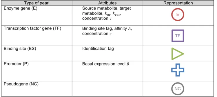
Each organism owns a circular single strand genome made of pearls being either functional or non coding. There are five types of pearls (table 1):

(1) Pearls coding for enzymes in the metabolic network (type E). Those pearls code for enzymatic reactions described by the following Michaelis-Menten equation:

(1) ![!] !" =

!!"#  .[!]  .[!]

!!![!] 𝑠, 𝑝   ∈ ℕ∗_{, 𝑘}

!"#∈  ℝ and 𝑘! ∈   ℝ!. 𝑠, 𝑝, 𝑘!"# and 𝑘! fully characterize the reaction. They are all encoded in the pearl’s 𝑛-tuple. [𝑠] and [𝑝] are the concentrations of the metabolites 𝑠 and 𝑝, and [𝐸] is the enzymatic (that is the 𝑛-tuple) concentration (here, we assume that the concentration of free enzymes [𝐸] is always equal to the total concentration [𝐸!], i.e. the concentration of combined enzymes [𝐸𝑆] is always close enough to zero. In this case, Michaelis-Menten dynamics are slightly biased, but it strongly reduces the number of equations to solve).

*

Genome GRN Metabolic network

Genome GRN Metabolic _network Growth rate (fitness)

Page 8 of 22 (2) Pearls coding for transcription factors (type TF). Each transcription factor 𝑖 owns an identification tag ∈ ℕ that specifies a binding site 𝑗, and an affinity 𝐴_!" for this binding site.

(3) Pearls coding for binding sites (type BS) specify which transcription factor may bind to them via their own identification tag  ∈ ℕ.

(4) Pearls coding for promoters (type P) determine where the transcription should start. Each promoter 𝑖 owns a basal expression level 𝛽_!.

(5) Non-coding pearls (type NC) constitute the non-coding part of the genome and drift in the 𝑛-tuple space. All type of pearl may become coding through the mutation process and a non-coding pearl can be restored with some probability into one of the four functional pearls.

Type of pearl Attributes Representation

Enzyme gene (E) Source metabolite, target metabolite, 𝑘!, 𝑘!"#,

concentration 𝑐

Transcription factor gene (TF) Binding site tag, affinity 𝐴, concentration 𝑐

Binding site (BS) Identification tag

Promoter (P) Basal expression level 𝛽

Pseudogene (NC)

Table 1 - Types of pearl in the basic network model. Note that this formalism simplifies the future extensions of the model. For instance, one could easily add “terminator” pearls or “Insertion Sequences” (IS) pearls. Binding sites directly flanking a promoter regulate its transcriptional activity. The enhancer site directly precedes the promoter (upstream pearls) and is made of one or more contiguous binding sites. The operator site directly follows the promoter (downstream pearls) and is also made of one or more contiguous binding sites. TFs that bind the enhancer site increase the transcriptional activity. On the opposite, TFs that bind the operator site down-regulate the promoter activity (see figure 4). As in R-aevol (Beslon et al., 2010b), a promoter has a basal level activity 𝛽, such that regulation sites are not mandatory. Note that this mode of regulation mimics the transcription dynamics of prokaryotes but is very different of what is observed in eukaryotes.

E

NC

Page 9 of 22

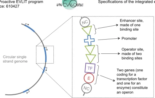
Figure 4 - Typical structure of a functional region in the genome. It starts with a promoter, possibly flanked by an enhancer site and/or an operator site (e.g. here, the enhancer site is made of one binding site, and the operator site is made of two binding sites). All contiguous E or TF pearls following the operator site are transcribed. The first pearl of another type interrupts the transcription (here a piece of non coding DNA). In this example the same unit of regulation controls the transcription of two coding pearls (an Enzyme and a Transcription Factor). Thus this functional region is an operon.

All TF or E pearls following an operator site (or following a promoter is no operator is present) are transcribed, thereby allowing for operons. Downstream of the operator site, any pearl other than TF or E makes the transcription stop. To be functional, the promoter can be flanked by binding sites or not, but TF or E pearls must immediately follow the regulation unit (enhancer site + promoter + operator site, see figure 5).

Figure 5 – (A) Three examples of pearls sequences coding for a functional region. The promoter can be flanked by binding sites or not, but TF or E pearls must immediately follow the regulation unit (enhancer + promoter + operator). (B) Two examples of non-functional pearls sequences. On the left, a non-coding pearl interrupts the transcription. On the right, the promoter is missing.

3.2. Mutational operators

The genome undergoes mutations during replication. When a point mutation occurs, the 𝑛-tuple of a pearl operates a jump in the tuples space by adding a 𝑛-dimensional random vector, even for NC pearls, which drift in the neutral space. A pearl can be unfunctionalized by a point mutation or

E NC NC Enhancer site, made of one binding site Promoter Operator site, made of two binding sites Two genes (one coding for a transcription factor and one for an enzyme) constitute an operon Circular single strand genome TF NC E NC NC E NC E E NC

Some functional combinations of pearls

functional region

(A)

Some non functional combinations of pearls

(B)

Page 10 of 22 during a rearrangement if it is located on a breakpoint. Non-coding pearls can also be restored into one or another functional type, however it is impossible to mutate directly from a functional type to another (see figure 6).

Figure 6 – Different mutation rates define the probability to switch from one pearl’s type to another. Functional types – binding sites (BS), transcription factors (TF), enzymes (E) and promoters (P) – can be unfunctionalized with probability pNC. A non-coding pearl can be restored to one type or another depending

on 4 mutations rates: pBS is the probability to become a binding site (resp. for pPROM, pE and pTF). In

summary, 5 mutation rates define the transition rates between pearl’s types.

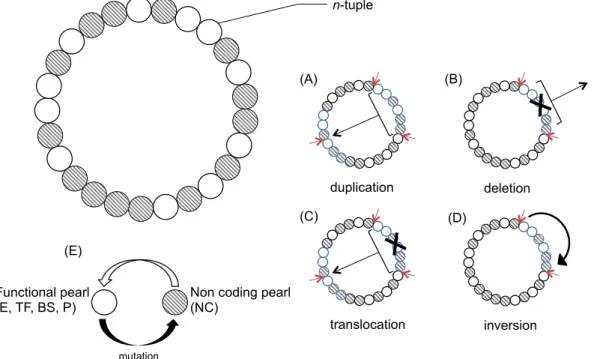
The genome also undergoes large chromosomal rearrangements: duplications, large deletions, inversions, and translocations. The various types of mutation can modify existing genes, but also create new genes, delete some existing genes, modify the length of the intergenic regions, modify gene order (as represented in the figure 7).

Figure 7 - Overview of the genome structure. The genome is a circular single-strand sequence of pearls, each coding for a 𝑛-tuple. At each replication, the genome undergoes mutations: point mutations, but also (A) large duplications, (B) large deletions, (C) translocations, (D) inversions. Red arrows symbolize breakpoints in the sequence. (E) point mutations and breakpoints can unfunctionalize or functionalize pearls.

NC E pNC$ pNC $ pNC$ p NC $ pBS $ pTF$ p_E$ p PROM $ TF n-tuple Functional pearl

(E, TF, BS, P) Non coding pearl (NC)

mutation duplication deletion translocation inversion (A) (B) (C) (D) (E)

Page 11 of 22

4. Regulation level

4.1. Basic features

The genetic regulation network is computed from the bag of 𝑛-tuples in three steps: (1) The activity 𝐴!(𝑡) of each binding site 𝑠 is:

(2) 𝐴_!(𝑡) =   _!𝑐_! 𝑡 𝐴_!"

with 𝑐!(𝑡) the concentration of the transcription factor 𝑗 at time 𝑡 and 𝐴!" the affinity of this transcription factor for the binding site 𝑠.

(2) From (1), we deduce the activity of the enhancer site 𝐸!(𝑡) and of the operator site 𝑂!(𝑡) flanking the promoter 𝑖:

(3) 𝐸! 𝑡 = !  ∈  !"!!"#$%!𝐴!(𝑡) 𝑂_! 𝑡 = _{!  ∈  !"#$%&!"!}𝐴_!(𝑡)

(3) Then, the transcription rate 𝑒! over time of the promoter 𝑖 is given by the Hill-like function:

(4) 𝑒_! 𝑡 =   𝛽_!  . !! !!! !!!!  . 1 +   ! !!− 1 !!! ! !!! !!!!

with 𝛽! the basal expression level of the promoter 𝑖, 𝑛 and 𝜃 being constant coefficients that determine the shape of the Hill function.

The transcription rate 𝑒! is applied to each E or TF pearl being controlled by the promoter 𝑖, such that each protein product (enzyme or transcription factor) has its own concentration regulated through a synthesis-degradation rule, depending on 𝑒_!:

(5) 𝑐!!!!0 =   𝛽!      

!" = 𝑒! 𝑡 − 𝜙𝑐!(𝑡)

where 𝜙 is a temporal scaling constant representing the protein degradation rate.

4.2. Adding noise in the genetic regulation network

In the cellular environment, the number of molecules of some reactant (enzymes or transcription factors) can be of low order (10-100 molecules). In this case, the stochastic effects due to reactant population size become predominant, as it is specially the case during gene expression (Elowitz et

al., 2002). Thus, the analysis of genetic regulation networks is complicated by fluctuations

associated with discrete reaction events in small-number reactant pools. Even if deterministic models are often sufficient to describe those processes, in many examples, they fail to capture some essential features of the underlying stochastic system (see Kaern et al., 2005 for a review). Several mathematical models deal with the fundamental stochastic nature of biochemical reactions, from discrete and stochastic models (SSA, Tau-leaping, CME) to continuous and stochastic ones (mainly the Chemical Langevin equation – CLE – see Gillespie et al., 2013 for a review. Unfortunately, even if discrete models are more realistic, they are computationally very

Page 12 of 22 costly and cannot be used in the case of an integrated model of evolution. We opted here for a continuous and stochastic model, by using stochastic differential equations (SDE). In this case, the assumption is made that the deterministic equations can be meaningfully separated from the stochastic fluctuations. The method consists in adding a random white noise term 𝜉(𝑡) to the deterministic equations describing protein concentrations (Scott, 2006). Many experimental studies agree with the fact that stochasticity in gene expression (SGE) mainly comes from stochasticity during transcription (Newman et al., 2006). Moreover, the structure of the promoter plays a major role in the noise strength (e.g. depending on the presence of a TATA box in eukaryotes). In prokaryotes, it is also recognized that promoters play a central role, and that the level of noise is somehow encoded in their structure and sequence (Roberts et al., 2011).

Let’s consider that the transcriptional noise is genetically encoded in the promoter. In the “pearls-on-a-string” formalism, this comes down to add a noise 𝜂 to the promoter type. 𝜂 mutates as all others attributes of the pearl, allowing for evolution of the SGE. Then, of each promoter 𝑖, the temporal dynamics of the transcription rate 𝑒! becomes (eq. 6):

(6) 𝑒! 𝑡 =   𝛽!  . ! ! !!!!!!!  . 1 +   ! !!− 1 !!!! !!!!!!! + 𝜉!(𝑡) with 𝜉! 𝑡 a random number drawn from the Gaussian distribution 𝒩(0, 𝜂!).

Since stochasticity is inevitable (the cell cannot escape the physical and chemical laws), a minimal noise 𝜂! exists such that 𝜂! ≥ 𝜂!.

5. Metabolic level

5.1. Basic features

Each pearl of type E (enzyme type) owns a 𝑛-tuple coding for one specific enzyme. In particular, the 4-tuple (𝑠, 𝑝, 𝑘!"#, 𝑘!), with 𝑠, 𝑝   ∈ ℕ∗, 𝑘!"# ∈  ℝ and 𝑘! ∈   ℝ!, completely describes the enzyme, 𝑠 and 𝑝 being the substrate and the product of the enzymatic reaction, and 𝑘!"# and 𝑘! being the constants of the corresponding Michaelis-Menten equation (eq. 7):

(7) ! ! !" =

!!"#× ! × !

!!! !  

With [𝑒] the concentration of the enzyme. If 𝑠   ≠  𝑝, the transition occurs in the cytoplasm of the cell. If 𝑠   =  𝑝, the enzyme becomes an inflowing or an outflowing pump depending on the sign of 𝑘_!"#. The entire set of enzymes gives rise to the cell metabolic network.

To sum up, we defined an artificial chemistry (Achem) {𝑆, 𝑅, 𝐴} where: • The set of molecules 𝑆 is the integer space ℕ∗,

• Each cell carries its own set of metabolic reaction rules 𝑅, defined by its genome. The 𝑛-tuple coding for the reaction rule is also considered as a molecule (an enzyme) with a concentration regulated by the genetic regulation network. However, at least in the first version of the model, the enzymes will not be able to modify each other.

Page 13 of 22 • The system of ordinary differential equations defining a cell’s metabolic network is

integrated using a continuous and deterministic method.

Thus, for each metabolic reaction rule 𝑟 ∈ 𝑅, the evolution of metabolite concentrations is described by the following equations:

(8) ![!] !" =   −   !!"#∗ ! ∗[!] !!![!] ![!] !" =   !!"#∗ ! ∗[!] !!![!]

5.2. Essential vs. non essential metabolites, metabolites toxicity,

cytoplasmic heritability

Essential and non-essential metabolites. As in real metabolism, some metabolic products are essential for the cell’s growth, and others are intermediate products or wastes. In the integrated model, prime numbers are considered to be essential metabolites: their production contributes to the growth and increases the probability to produce offspring. This contribution is simply the sum of all essential metabolite concentrations.

Metabolites toxicity. As in real metabolism too, over producing metabolites can lead to toxicity for the cell. Hence, the model includes toxicity thresholds for essential and non-essential metabolites. Overreaching the toxicity threshold kills the cell.

Cytoplasm heritability. During replication, daughter cells share cytoplasmic content at division. This behaviour can lead to very specific behaviour, especially if some metabolites are co-enzymes of transcription factors, as it will be explained below.

6. Coupling the genetic and the metabolic networks

Bacteria are able to sense their environment by detecting the presence of a particular molecule or signal, and to give an appropriate answer by updating their gene expression profile. A famous example of this behaviour is the lactose operon, described for the first time by François Jacob, Jacques Monod and André Lwoff.

The lactose operon is made of three genes (lacZ, lacY and lacA) that are controlled by one promoter flanked by an operator. Another gene, lacI, codes for a transcription factor which inhibates the operon by binding on the operator. LacI is always expressed and its concentration in the cytoplasm is almost constant. However its conformation, hence its affinity for the operator is (indirectly) modified by lactose. In absence of lactose, lacI is active and down-regulates lactose operon expression by binding on the operon. If lactose is present, it represses lacI activity (by binding on it). In this case, lactose operon is expressed and the cell is able to metabolize lactose (see figure 8).

Page 14 of 22

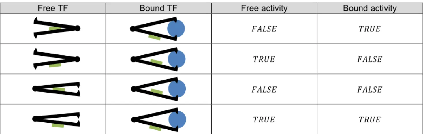
Figure 8 - (From http://apps.cmsfq.edu.ec/biologyexploringlife/) The lactose operon is inactive in the absence of lactose (top) because a repressor blocks attachment of RNA polymerase to the promoter. With lactose present (bottom), the repressor is inactivated, and transcription of lactose-processing genes proceeds. Co-enzymes can repress or activate transcription factors activity (they are repressors or activators). This very important biological feature is introduced in the integrated model by adding three elements to the transcription factor type (TF):

• A co-enzyme identification tag (in the metabolic space ℕ∗), • A free activity (true or false),

• A bound activity (true or false).

A metabolite 𝑚   ∈ ℕ∗  _{can bind to the TF as a co-enzyme, and be a repressor or an activator. A TF} has two conformations: one when the TF is free, and another when a co-enzyme binds to it. This behaviour is represented in table 2 by a structure with two arms linked by a pivotal point. The active site of the TF is located on one arm, and its exposure depends on the equilibrium state (or conformation) of the structure. Two configurations exist: one when the TF is free, another when a co-enzyme bind to the TF thanks to anchoring points located at arms end. The combination of the free activity and the bound activity gives rise to four type of behaviours, as described in table 2. (1) If the TF has no free activity, and has a bound activity, the co-enzyme acts as an activator, (2) If the TF has free activity, and has no bound activity, the co-enzyme acts as a repressor, (3) If the TF has no free activity neither bound activity, the TF is not active.

(4) Finally, if the TF has free activity and bound activity, the co-enzyme has no effect. The TF is always active, whenever a co-enzyme binds to it or not.

Page 15 of 22

Free TF Bound TF Free activity Bound activity

𝐹𝐴𝐿𝑆𝐸 𝑇𝑅𝑈𝐸

𝑇𝑅𝑈𝐸 𝐹𝐴𝐿𝑆𝐸

𝐹𝐴𝐿𝑆𝐸 𝐹𝐴𝐿𝑆𝐸

𝑇𝑅𝑈𝐸 𝑇𝑅𝑈𝐸

Table 2 - The TF is represented in black, its active site (the part which allow the TF to bind on the binding site) being represented in green. Depending on free and bound activities, the co-enzyme (in blue) acts as an activator or a repressor, and the active site is free to bind to the binding site or not.

Let’s 𝑐!(𝑡) be the concentration of the TF 𝑖 at time 𝑡 and 𝑐𝑜𝐸!(𝑡) the concentration of its co-enzyme. Depending on the state of the free activity 𝐴_!! and the bound activity 𝐴!_!, the concentration of the TF 𝑖 that is active  𝑎_!(𝑡) at time 𝑡 is:

(9) 𝑎!(𝑡) = 𝑚𝑖𝑛 𝑐_! 𝑡 , 𝑐𝑜𝐸_!(𝑡) , 𝐼𝐹(  𝐴_!!  _{𝑖𝑠  𝑓𝑎𝑙𝑠𝑒    𝐴𝑁𝐷    𝐴} ! !  _{𝑖𝑠  𝑡𝑟𝑢𝑒      )} 𝑚𝑎𝑥 𝑐_! 𝑡 − 𝑐𝑜𝐸_! 𝑡 , 0 , 𝐼𝐹(  𝐴_!!  _{𝑖𝑠  𝑡𝑟𝑢𝑒        𝐴𝑁𝐷    𝐴} ! !  _{𝑖𝑠  𝑓𝑎𝑙𝑠𝑒  )} 𝑐!(𝑡), 𝐼𝐹(  𝐴!!  𝑖𝑠  𝑡𝑟𝑢𝑒        𝐴𝑁𝐷    𝐴!!  𝑖𝑠  𝑡𝑟𝑢𝑒      ) 0, 𝐼𝐹(  𝐴_!!  𝑖𝑠  𝑓𝑎𝑙𝑠𝑒    𝐴𝑁𝐷    𝐴_!!  𝑖𝑠  𝑓𝑎𝑙𝑠𝑒  )

7. Population and environment levels

Open-endedness requires individuals to interact with each other. However, inter-individual interactions must not occur at the whole population level (i.e. all individuals interacting with all individuals), otherwise there is a strong risk to reduce the variability between individuals. That is why, following the work of P. Hogeweg’s group, the integrated model uses a spatial structure. Individuals are dispatched on a 2D lattice of size 𝑊. 𝐻  (with 𝑊 the width and 𝐻 the height of the lattice), each grid cell containing at most one individual. The physical environment is also described at the lattice level: each lattice cell contains a list of free metabolites, each with its concentration level. Those free metabolites diffuse and degrade, both processes being controlled by two parameters: the diffusion rate 𝐷 and the degradation rate 𝐷!.

• Diffusion: at each time step, a proportion of the free metabolites of a given cell i are spread to its Moore neighbourhood (the 8 surrounding cells). This proportion will be controlled by the diffusion parameter 𝐷.

• Degradation: at each time step, a proportion of the free metabolites of a given cell i are removed. This proportion is controlled by the degradation parameter 𝐷_!.

Individuals compete for the free metabolites and to produce offspring in empty cells. Individuals interact with their local environment by pumping metabolites in and out and releasing their content at death (see below).

Page 16 of 22 The formalism presented above allows for several outcomes. First, population size is variable. Depending on growth rate, lattice size, and interactions between individuals, simulations can lead to steady state, but also to oscillations or even extinctions. Second, since individuals can interact with their surroundings via intake and release of metabolites, interactions between individuals can emerge such as necrophagy, public goods sharing, arms race by releasing toxic metabolites, and so on.

In order to vary the strength of the spatial structure, a random fraction 𝑚𝑖𝑔 of organisms and free metabolites can be swapped at each time step. To do so, pairs of lattice cells are randomly chosen and their contents are swapped. Depending on the 𝑚𝑖𝑔 value, one can vary the population structure from well-mixed (𝑚𝑖𝑔 = 1) to perfectly local (𝑚𝑖𝑔 = 0). Moreover, some metabolites can also be artificially maintained at a constant concentration, be regularly provided locally or globally in the environment or, on the opposite, be regularly washed-out from the environment. Thus, various real experimental setups can be mimicked, including serial plates or chemostat (Mozhayskiy & Tagkopoulos, 2012). Similarly, some individuals can be regularly picked up in the environment to seed a new colony, thus mimicking a mutation accumulation experiment. All these optional features will be useful for further experiments in WP3 and to mimic the wet experiments of WP1 (figure 9). In order for the simulation to be computationally tractable, a minimum concentration threshold is defined. Bellow this threshold a given metabolite is considered absent from the local environment.

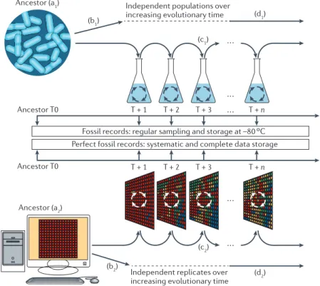
Figure 9 – Parallel in vivo (top) and in silico (bottom) experimental evolution. The experiments conducted in vivo are mimicked in the computational framework. Figure from (Hindré et al., 2012).

Nature Reviews | Microbiology

Independent populations over increasing evolutionary time

Independent replicates over increasing evolutionary time

Ancestor (a₁) Ancestor (a₂) (b₁) (b₂) T + 1 T + 2 T + 3 T + n T + 1 Ancestor T0 Ancestor T0 T + 2 T + 3 … … … … … T + n (c₁) (c₂) (d₁) (d₂)

Fossil records: regular sampling and storage at –80 ºC Perfect fossil records: systematic and complete data storage

Variability

The potential or propensity of the phenotype to vary (whether or not it actually does in the present population or sample). This depends on the rates and patterns of mutation and recombination, and on the genotype–phenotype map. Fitness

An integrated measure of the relative survival and reproductive rate of genotypes in a given environment. Evolvability

The potential or propensity of the phenotype to vary in a possibly adaptive manner.

adaptation, as well as global laws that link evolutionary processes and organismal structure. However, using such an evolutionary perspective is difficult, mainly because the relevant events that resulted in the present organismal structure occurred at some unknown time in the past, in unknown conditions and with unknown constraints. Thus, specific tools are necessary to directly observe evolutionary dynamics and relate these events to the real conditions in which they occur.

The past three decades have seen the emergence of experiments that are designed to reproduce evolution

in controlled conditions in the laboratory2 _{and, more}

recently, on a computer3_{. Laboratory in vivo}

evolu-tion experiments focus on the single most important, integrative and complex phenotype of all: fitness. They allow rigorous connections to be made between genetic changes and phenotypic outcomes in a complex adaptive

system, such as a bacterial cell. The adaptive muta-tions that are discovered during evolution experiments are often subtle in their phenotypic effects and there-fore different from those observed in more traditional genetic studies, in which genes are typically knocked out and selective screens usually rely on extreme ‘plus or minus’ phenotypes. In parallel — and often inde-pendently — evolution experiments have also been conducted on artificial, non-living substrates. For two decades, computer simulations and in silico experimen-tal evolution approaches have been developed, in which

artificial organisms (so-called digital organisms_{) evolve in}

a computational environment. In these digital experi-ments, practitioners are aware of all possible evolution-ary events (including variations that appear and are not further selected for), and the experiments are highly reproducible, and can be carried out in multiple con-texts and under multiple evolutionary conditions. In vivo experimental evolution enables a better understanding of the pace of evolution and its main features in living

organisms2,4_{. When combined with molecular biology}

and high-throughput technologies, it also allows pheno-typic variations to be related to the molecular events that

occurred in the course of the experiment5–7_{. In silico}

experimental evolution can bypass species-specific traits and generate more general observations.

Here, we review in vivo and in silico evolution experi-ments for bacteria; although there have also been reports

of these experiments for viruses8,9 _{and higher eukaryotes}

such as Drosophila melanogaster10_{, they are not discussed}

in this Review. We focus especially on new insights from experimental evolution that link global microbial pheno-types (such as physiology and behaviour) with molecular and regulatory observations. We also discuss the limits of experimental evolution, as well as future perspectives, including the need for closer collaboration between researchers using in vivo and in silico approaches.

and experimental evolution

Biological systems emerge through Darwinian evolution, which is characterized by random genetic modifications

followed by selection of well-adapted individuals11_{. This}

combination of ‘chance and necessity’ can be stud-ied efficiently by propagating organisms in controlled

environments (FIG. 1)_{. This strategy, called}

experimen-tal evolution, provides complementary advantages to

most classical genetic studies (BOX 1)_{. Owing to their}

short replication times, large populations and easy

stor-age2_{, microorganisms are excellent candidates for use in}

experimental evolution4,6,7_{(TABLE 1). Replicate}

popula-tions have been propagated from microbial ancestors over different evolutionary timescales, from tens to tens of thousands of generations, and under diverse environ mental conditions. These different environments impose selection for changes in either specific pheno-types (including growth in the presence of inducible or non-native substrates, and resistance to stresses such as antibiotics, atypical pH or temperature) or broad pheno-types (such as growth in the presence of preferred

car-bon sources12–17 _{or fluctuating levels of resources}18_{; social}

behaviours, including differentiation and the production

Figure 1 | microbial and evolution experiments. Ancestral microbial

organisms (top) or artificial organisms (bottom) are propagated in defined wet or computer environments, respectively. The main advantage in these experiments is the availability of an ancestor and the evolved populations that are sampled throughout evolution. All living and artificial organisms can be frozen or stored in databases, respectively, and revived at any time for further analyses. Many parameters can be varied.

, the ancestor (a₁) can be any microorganism, the only constraint being its ease of

cultivation; ancestral digital organisms (a₂) can be randomly constructed, or designed to

have capabilities such as replication or minimal metabolism. The number of replicate

cultures (b₁ and b₂) can be varied, leading to independent populations derived from the

common ancestor. , culture conditions can be varied, including the media, the

physical parameters, the structure of the environment (batch or chemostat culture; heterogeneous or homogeneous environments), the effective population size and the

bottlenecks at each transfer (c₁). , almost all parameters can be tested independently

or in combination, including mutation rates, mutation biases and selection strength,

which define the way in which the transfer (c₂) is carried out. The total duration (d₁)

and sampling times of experiments can be varied; experiments classically

run for hundreds of thousands of generations (d₂).

R E V I E W S

NATURE REVIEWS |MICROBIOLOGY VOLUME 10 | MAY 2012 | 353

Page 17 of 22 To summarize, the environment level is characterized by the following parameters:

• Environment size 𝑊. 𝐻 (𝑊. 𝐻 thus being the maximal carrying capacity2 of the environment),

• Diffusion coefficient 𝐷, • Degradation rate 𝐷!,

• Metabolites inflow 𝐼! (for each metabolite 𝑖), • Metabolites outflow 𝑂! (for each metabolite 𝑖), • The migration coefficient 𝑚𝑖𝑔,

• The minimum concentration threshold.

Note that the dynamics of inflow/outflow can be constant (i.e. applied at each time step) or time dependent.

At a given time t each lattice cell of coordinate (𝑥, 𝑦) is characterized by: • The individual that occupies the cell (possibly null)

• The list of free metabolites that are available and their concentrations 𝐶!(𝑡)

Given the parameters of the environment, the dynamics of a free metabolite 𝑖 in a lattice cell 𝑘 is then given by (𝐶!,! being the concentration of metabolite 𝑖 in the lattice cell 𝑗):

(10) 𝐶!,! 𝑡 + 1 = 𝐶!,! 𝑡 − 𝐷!𝐶!,! 𝑡 +   !  !"  !"#$!!"#$%𝐷𝐶!,! 𝑡 − 8𝐷𝐶!,!(𝑡) + 𝐼!(𝑡) − 𝑂!(𝑡)

7.1. Interactions between individuals

The environment level described above enables interactions between individuals through modification of a shared environment. For these interactions to be efficient and effectively lead to complex evolutionary dynamics and open-endedness, individuals must be able to structure their environment and the environment of their neighbours, thus influencing their “life” and evolutionary fate. To do so, we provide the individuals with three properties:

(1) The ability to release metabolites in the environment, (2) The ability to intake metabolites from their environment,

(3) The possibility to indirectly modify the inner metabolites concentration of their neighbours, due the permeability of the cell membranes.

These properties are achieved through special proteins called pumps. As explained above in our artificial chemistry, E pearls encode enzymes that transform a substrate (actually an integer 𝑠 ∈ ℕ∗₎ into another one, the product (another integer 𝑝 ∈ ℕ∗_{), with a specific rate but we consider that the} enzymes for which the substrate and the product are equal (i.e. 𝑠   =  𝑝) are inflowing or outflowing pumps for the metabolite 𝑠. The orientation of the pump (inflow or outflow) and its efficacy are specified by the reaction constants encoded in the 𝑛-tuple. Using such pumps, the individuals are able to control their cytoplasm composition and to maintain their internal homeostasis.

2 _{The actual carrying capacity may depend on the species needs and on the metabolites available in the}

environment. In a complex situation where the environment contains different co-evolving species, the carrying capacity of each species may depend on the metabolites released by the other ones and on the dynamic of metabolites inflow/outflow.

Page 18 of 22 The pumps are important mechanisms for the cell to maintain a stable metabolic activity. However, by themselves, they do not allow for complex cell-to-cell interactions since each individual can fully and autonomously control its internal composition. That is why we added two mechanisms allowing for resource cycling and complex cell-to-cell interactions:

• “Necrophagy”: each time an individual dies, all the metabolites it contains are released in the local environment and start diffusing on the grid. This mechanism will lead for a progressive complexification of the environment as long as evolution creates more and more complex individuals.

• “Permeable membrane”: the cell membranes are not perfect barrier for metabolites. As well as metabolites diffuse on the environment grid, they diffuse from the grid cell (i.e. the local physical environment of the individual) to the individual itself with a diffusion coefficient 𝐷!. At each time step, a fraction 𝐷! of the metabolites diffuse through the cell membrane, resulting in a progressive balancing of the metabolites concentrations in the environment and in the cell. Thus, pumps are active mechanisms that the cell can use to maintain an internal concentration different from the external one3_{. Consequently, a metabolite actively}

released by an individual in its environment will diffuse to the neighbouring lattice cells (with diffusion coefficient 𝐷) and to the individuals that “live” there (with a diffusion coefficient 𝐷!), possibly perturbing their internal metabolic activity, unless these individuals have evolved mechanisms to protect themselves against these perturbations.

These two additional mechanisms are likely to initiate complex dynamics at the ecosystem level (creation of a trophic network, niche construction…) and at the cell-to-cell level (release of public good or, on the opposite, of bacterial toxins).

7.2. Additional features

In order to increase the level of complexity and realism of the environment, some features could be added to the current specifications, for example:

• Allow for the diffusion of enzymes, TF and/or plasmids in the environment, • Allow for the release of DNA in environment at death,

• Define some metabolites that behave like toxins, • Allow for bacterial conjugation or transformation.

8. General algorithm

Population of organisms are evolved in a dedicated program that controls the variation-selection process. At each simulation time step, organisms are evaluated and either killed, updated or replicated depending on their current state and on the states of the other organisms living in their Moore neighbourhood. In particular, organism’s replication is determined by its relative fitness and by the availability of a gap in its Moore neighbourhood.

3 _{Depending on the 𝐷}

! value, the pumps will precisely control the internal composition of the cytoplasm

(𝐷!= 0) or they will have no effect (𝐷!= 1). In between, pumps and membrane permeability will balance

Page 19 of 22 (1) Death probability follows a Poisson law of parameter 𝑝!"#$!, defined at the beginning of the simulation. At death, organism’s cytoplasm is released in the local environment (i.e. metabolite concentrations) and can feed other organisms.

(2) If the organism do not die and is unable to divide (e.g. because there is no gap in its neighbourhood), its state is updated. Genetic regulation network and metabolic network are updated, and the score of the cell is computed by summing essential metabolites concentrations. In details, equations 2, 3, 4, 5 (or 6), 8 and 9 are solved via an ODE numerical solver, using the explicit embedded Runge-Kutta-Fehlberg method. Equation 10 and the score are computed directly using Euler’s method.

(3) For each gap, a competition occurs in the Moore neighbourhood to select the replicating individual, depending on the differences of fitness. Each organism 𝑖 is allowed to compete if 𝑠𝑐𝑜𝑟𝑒!>  Θ ∗ 𝑠𝑐𝑜𝑟𝑒!"# with 𝑠𝑐𝑜𝑟𝑒! the score of the organism 𝑖, Θ ∈ [0,1] fixed at the beginning of the simulation, and 𝑠𝑐𝑜𝑟𝑒!"# the maximum score in the population. The fitness 𝑤! of each individual 𝑖 is then computed as following:

(11) 𝑤! = _!"#$%!"#$%!

!"#

!

with 𝑝 a positive factor increasing the selection pressure. To avoid biases, gaps are explored randomly.

9. Conclusion

The integrated model has been developed to study highly complex evolution dynamics. To do so, we followed the principles of Artificial Life by mimicking biological evolution in a computer-world. The way such a complex model is implemented, optimized and tested is of primary importance. Like for every modelling process, inevitable simplifications have been made. As a consequence, we cannot keep the resolution applied in previous models (e.g. the detailed genomic structure in

aevol, or the complex equations driving binding sites dynamic in the virtual cell model). However,

like in numerical weather predictions, details of subprocesses can be neglected in the face of the whole system evolution, understood that simplifications no dot significantly affect higher level predictions. To observe evolution of evolution, interactions between objects are probably more important than their nature (in vivo or in silico) and the details of their representation. For instance, our representation of the genome is coarse-grained compared to aevol, however, main outcomes of indirect selection on the genome structure are maintained (non coding DNA amount, number of genes, …). We also strongly simplified the transcriptional noise model, as well as equations driving transcription factors and binding sites activity. The artificial chemistry is simplified, since chemical basis of the reactions has been abstracted (e.g. the absence of chemical bonds or complex molecules).

But, as illustrated in the figure 10, we think that an integrated model of evolution is able to give a big picture of how evolution shapes a complex system, even if the representation of each interacting entity is smoothed. Our approach is quite similar to real experimental approaches (Beslon, 2008). Our work includes three main steps:

• Do parametric exploration and identify parameter variations having (or not) significant effects on evolutionary dynamics,

Page 20 of 22 • Build experimental protocols to study the effect of the identified parameters.

• Compare in vivo and in silico results, offer new hypothesis and insights on a particular subject, give guidance on which data are most important to gather experimentally.

Using the simulation as an experimental system is “an efficient way to mimic complex systems and

manipulate them in ways that would be impossible, too costly or unethical to do in natural systems”. (Peck, 2004). Indeed, the way we represented biological processes in the integrated

model fills a little more the gap between in vivo experimental evolution and in silico experimental evolution. A system biology and artificial life progressively come closer and tend to explore similar objects with a common vocabulary. This tendency is strongly lightened in the EvoEvo project, since we also built the model in agreement with the work of our partners in experimental biology (UJF and CSIC).

Figure 10 – Let’s suppose that one can only have a closer look to this painting of Vincent Van Gogh (“Champ de blé aux corbeaux”, 1890), famous for unfortunate reasons. Probably one will be able to identify a black bird, but very poorly detailed. Other shapes (mainly brush strokes) will remind one grass, or even wheat with some imagination. One will probably assert this is abstract art. In reality, details of small entities don’t matter if our interest focuses on their interactions. Now, if one can see the global picture, one will observe that grass only grows on field borders, that birds behave collectively and probably eat wheat, and that something drawn mud trails. Even more, if one could have the complete history of this landscape, one would understand a lot more, e.g. that grass do not grow on trails because workers crush it, neither in fields because wheat monopolizes water resources. Our integrated model will give us the same metaphoric picture of evolutionary dynamics, in order to study the emergence of complex EvoEvo strategies.

Page 21 of 22

10. References

[Beslon, 2008] Beslon, G. (2008) Apprivoiser la vie: Modélisation individu-centrée de systèmes biologiques complexes. Habilitation à Diriger des Recherches, INSA-Lyon. Available on the

Internet: http://liris.cnrs.fr/Documents/Liris-3717.pdf (accessed, December 2014).

[Beslon et al., 2010a] Beslon, G., Parsons, D. P., Sanchez-Dehesa, Y., Peña, J.-M. and Knibbe, C. (2010) Scaling laws in bacterial genomes: A side-effect of selection of mutational robustness?

BioSystems, 102(1):32-40.

[Beslon et al., 2010b] Beslon, G., Parsons, D. P., Peña, J.-M., Rigotti, C. and Sanchez-Dehesa, Y. (2010) From digital genetics to knowledge discovery: Perspectives in genetic network understanding. Intelligent Data Analysis journal, 14(2):173-191.

[Crombach & Hogeweg, 2008] Crombach, A. and Hogeweg, P. (2008) Evolution of evolvability in gene regulatory networks. PLoS computational biology, 4(7):e1000112.

[Cuypers & Hogeweg, 2012] Cuypers, T. D. and Hogeweg, P. (2012) Virtual genomes in flux: an interplay of neutrality and adaptability explains genome expansion and streamlining. Genome

biology and evolution, 4(3):212-229.

[Dittrich et al., 2001] Dittrich, P., Ziegler, J. and Banzhaf, W. (2001) Artificial Chemistries - A Review. Artificial Life, 7(3):225-275.

[Gillespie et al., 2013] Gillespie, D. T., Hellander, A. and Petzold, L. R. (2013) Perspective: Stochastic algorithms for chemical kinetics, The Journal of chemical physics, 138:170901.

[Elowitz et al., 2002] Elowitz, M. B., Levine, A. J., Siggia, E. D. and Swain, P. S. (2002) Stochastic gene expression in a single cell. Science, 297(5584):1183-1186.

[Hindré et al., 2012] Hindré, T., Knibbe, C., Beslon, G. and Schneider, D. (2012) New insights into bacterial adaptation through in vivo and in silico experimental evolution. Nature Reviews

Microbiology, 10(5):352-365.

[Kaern et al., 2005] Kærn, M., Elston, T. C., Blake, W. J. and Collins, J. J. (2005) Stochasticity in gene expression: from theories to phenotypes. Nature Reviews Genetics, 6(6):451-464.

[Knibbe et al., 2007a] Knibbe, C., Mazet, O., Chaudier, F., Fayard, J.-M. and Beslon, G. (2007) Evolutionary coupling between the deleteriousness of gene mutations and the amount of non-coding sequences. Journal of Theoretical Biology, 244(4):621-630.

[Knibbe et al., 2007b] Knibbe, C., Coulon, A., Mazet, O., Fayard, J.-M. and Beslon, G. (2007) A long-term evolutionary pressure on the amount of noncoding DNA. Molecular Biology and

Evolution, 24(10):2344-2353.

[Mozhayskiy & Tagkopoulos, 2012] Mozhayskiy, V. and Tagkopoulos, I. (2013) Microbial evolution in vivo and in silico: methods and applications. Integrative Biology, 5(2):262-277.

Page 22 of 22 [Newman et al., 2006] Newman, J. R., Ghaemmaghami, S., Ihmels, J., Breslow, D. K., Noble, M., DeRisi, J. L. and Weissman, J. S. (2006) Single-cell proteomic analysis of S. cerevisiae reveals the architecture of biological noise. Nature, 441(7095):840-846.

[Peck, 2008] Peck, S. L. (2004) Simulation as experiment: a philosophical reassessment for biological modeling. Trends in Ecology & Evolution, 19(10):530-534.

[Roberts et al., 2011] Roberts, E., Magis, A., Ortiz, J. O., Baumeister, W. and Luthey-Schulten, Z. (2011) Noise contributions in an inducible genetic switch: a whole-cell simulation study. PLoS

computational biology, 7(3):e1002010.

[Scott, 2006] Scott, M. (2006) Tutorial: Genetic circuits and noise. Available on the Internet: http://www.math.uwaterloo.ca/mscott/NoiseTutorial.pdf (accessed, December 2014).

[Soyer & O’Malley, 2013] Soyer, O. S. and O'Malley, M. A. (2013) Evolutionary systems biology: What it is and why it matters. BioEssays, 35(8):696-705.