The Areal Reduction Factor (ARF) : a multifractal analysis

4

The Areal Reduction Factor (ARF) a

Multifractal Analysis

by

Andreas Langousis

Diploma of Civil and Environmental Engineering (2003) National Technical University of Athens.

MASSACHUSETTS I S OF TECHNOLOGy

FEB 2

4 2005

LIBRARIES

Submitted to the Department of Civil and Environmental Engineering

in partial fulfillment of the requirements

for the degree of

MASTER OF SCIENCE IN CIVIL AND ENVIRONMENTAL ENGINEERING

at the

MASSACHUSETTS INSTITUTE OF TECHNOLOGY

@ 2005 Massachusetts Institute of Technology. All rights reserved

Signature of Author..

...

Department of Civil and Environmental Engineering October 6, 2004

Certified by...

Professor of Civil and Environmetal Engineering

ksl

I

I

Accepted by...

I...

The Areal Reduction Factor (ARF) a Multifractal

Analysis

by

Andreas Langousis

Submitted to the Department of Civil and Environmental Engineering on October 6, 2004 in partial fulfillment of the requirements

for the Degree of Master of Science in Civil and Environmental Engineering.

Abstract

The Areal Reduction Factor (ARF) ?7 is a key parameter in the design for hydrologic extremes. For a basin of area A, r(A, D, ) is the ratio between the area-average rainfall intensity over a duration D with return period T and the point rainfall intensity for the same D and T. Besides depending on A, D and possibly T, the ARF is affected by the shape of the basin and by a number of seasonal, climatic and topographic characteristics. Another factor on which ARF depends is the advection velocity, vad, of the rainfall features. Commonly used formulas and charts for the ARF have been derived by smoothing or curve-fitting empirical ARFs extracted from raingauge network records.

Here we derive some properties of the ARF under the assumption that space-time rainfall is exactly or approximately multifractal. We do so for various shapes of the rainfall collecting region and for vad = 0 and vadA 0.

When vad = 0, a key parameter in the analysis is the ratio ures = vres/Ve between the "response

velocity" vres = LID, where L is the maximum linear dimension of the region, and the "evolution velocity" ve = Le/De, where Le and De are the characteristic linear dimension and characteristic

duration of organized rainfall features.

The effect of vad # 0 depends on the shape of the region. For highly elongated basins, both the direction and magnitude of advection are influential, whereas for regular shaped regions only the magnitude vad matters.

We review ways in which rainfall has been observed to deviate from exact multifractality and models that capture such deviations. We show how the ARF behaves when rainfall is a bounded cascade in space and time. We also investigate the effect of estimating areal rainfall from raingauge network measurements. We find that bounded-cascade deviations from multifractality

and sparse spatial sampling distort in similar ways the scaling properties of the ARF.

Finally we show how one can reproduce various features of empirical ARF charts by using multifractal and bounded cascade models and considering the effects of sparse spatial sampling.

Thesis Supervisor: Daniele Veneziano

Dedicated to my father, my mother, and my brother.

Acknowledgments

Reaching the end effort, I would like to acknowledge all those who contributed and provided the basis for this work.

First of all I would like to thank my professor and friend Daniele Veneziano for his contributions to my thesis, and the time he spent working with me providing continuous support during this academic year. Daniele Veneziano is not only an outstanding professor and researcher; he is also a most understanding and helpful person. If it wasn't for him, I doubt this thesis would have been finished.

By no means can I forget my former research supervisor, professor and best friend Demetris Koutsoyiannis, who introduced me to the magic world of stochastic processes. I entered this field by taking his course "Stochastic Hydrology" at the National Technical University of Athens. By the end of the course I was addicted to stochastic processes and started working with him on stochastic modeling.

Of course, I cannot omit to acknowledge some persons that truly marked my life by providing me the basis in mathematics and engineering. My high-school teachers Stavros Drosakis and Demetris Nasiopoulos taught me that mathematics is not only an interesting game but also an attractive way of thinking.

Nikolaos Ioakimidis, Professor of Applied Mathematics at the Polytechnic School of University of Patras, is the person that academically fended for me most during my first year of graduate studies in the University of Patras. I still remember his words: "Studying is good only ifyou

know when to stop", which I never followed.

George Christodoulou, Professor of Applied Hydraulics at the National Technical University of Athens, Andreas Andreadakis, Director of the Sanitary Engineering Laboratory at the National Technical University of Athens, and the Hydraulic Engineers Jack Gabrielidis and Tilemahos Papathanasiadis are the persons that I have to thanks most for becoming a Hydraulic Engineer. Finally I owe a great thanks to my father, my mother and my brother who always supported me and never stopped believing in me.

Special Acknowledgments: This work was supported in part by the Department of Civil and Environmental Engineering of Massachusetts Institute of Technology under Schoettler

Fellowship, in part by the National Science Foundation under Grant No. EAR-0228835, and in

part by "Alexander S. Onassis" Public Benefit Foundation under Scholarship No. F-ZA 054/2004-2005.

Cambridge, October 2004 Andreas Langousis

Table of contents

A bstract...2

A cknow ledgm ents...4

Introduction ... 6

1 Literature review ... 9

1.1 The Areal Reduction Factor (ARF)... 9

1.2 Empirical methodologies for estimating ARFs...10

1.3 Semi-theoretical methodologies for estimating ARFs...14

2 Extremes of multifractal rainfall in time...21

2.1 Cramer's Theorem for sums of independent random variables...21

2.2 Extremes of bare and dressed multifractal cascades...23

2.3 Scaling properties of the intensity duration frequency curves...26

2.4 Conclusions and comments...31

3 Extremes of multifractal rainfall in time and space... 32

3.1 Extremes of Multifractal Space-Time Rainfall for vad = 0... 33

3.2 The Effect of Advection...47

3.3 Numerical validation...55

3.4 Velocity parameters... 62

3.5 Com m ents... 67

4. Imperfect scaling of rainfall, sparse sampling and their effects on the ARF...68

4.1 Observed deviations of rainfall from multifractality... 70

4.2 Raingauge network density and deviations from multifractality...83

4.3 Effect of bounded cascade modeling and sparse sampling on the ARF...84

5. Application to the N.E.R.C. curves...91

5.1 N.E.R.C.'s ARF curves...91

5.2 Behavior of the ARF in Figure 5.2... 95

5.3 Numerical reproduction of the N.E.R.C. ARF results...97

5.4 Conclusions and comments...102

6. C onclusions...104

R eferences...110

Introduction

In hydrological risk analysis and design, knowledge of the probability of rainfall extremes is essential. For example, in reservoir design and flood estimation one is interested in rainfall intensities averaged over an area A and a duration D, with a given return period T. These intensities are provided by the so-called Intensity Duration Area Frequency (IDAF) curves.

Direct estimation of the IDAF curves from rainfall records is a difficult task, because it is rare to have extensive records from spatially dense pluviometric networks or radar. For A = 0 (precipitation at a point), the IDAF curves reduce to the familiar Intensity Duration Frequency (IDF) curves.

Since it is relatively easy to estimate the IDF curves using long rainfall records from single pluviometric stations, a convenient and commonly used way of estimating the IDAF curves is to multiply the IDF values by an Areal Reduction Factor (ARF). This factor is defined as the ratio of the rainfall intensity averaged over area A and duration D with return period T, and the rainfall intensity at a point for the same D and T.

The ARF increases with decreasing area A, approaching unity as A tends to zero. Also, the ARF increases as duration D increases. The effect of the return period T on the ARF is not clear. N.E.R.C. (1975) finds a weak dependence of the ARF on T (ARF slightly increases as T decreases), whereas other researchers (Bell, 1976; Asquith et al., 2000; De Michele et aL., 2001) find that the ARF is largely influenced by T. Specifically, they find that the ARF decreases with increasing T, and that its dependence (see above) on A and D becomes more pronounced for larger values of T.

A number of empirical formulas have been proposed for the estimation of the ARF from rainfall records. Most of them consider the ARF to be independent of the return period T. ARF curves for general use have also been proposed. These curves give the ARF as a function of only

A and D, and therefore assume negligible dependence on the return period T, geometry of the

basin, and climatic conditions.

Several studies have tried to derive the ARF, IDF or IDAF curves using semi-theoretical probabilistic models of rainfall (Roche, 1966; Rodriguez-Iturbe and Mejia, 1974; Bacchi and Ranzi, 1996; Sivapalan and B16schl, 1998; Asquith and Famiglietti, 2000). Most of them incorporate the spatial correlation structure of rainfall, as well as semi-theoretical functions and

constants that have to be inferred from data. In practice, estimation of those quantities is often inaccurate.

Since rainfall data rarely allow direct estimation of rainfall intensities over the range of areas, durations and return periods of practical interest, one way to make the inference of rainfall extremes more robust is to use theoretical model-based results. Multifractal models provide a good representation of space-time rainfall fields (Lovejoy and Schertzer, 1995; Gupta and Waymire, 1993; Deidda, 2000) and possess scale-invariance properties that may be at the root of certain power-law behaviors observed in empirical ARF curves. Therefore, it is attractive to use the theory of multifractality to explain the behaviour of rainfall extremes and extend the empirical ARFs beyond the range of A, D and T covered by the data. For example, Bendjoudi et

al. (1999) and Veneziano and Furcolo (2002a) used multifractal rainfall models to determine the

scaling properties of the IDF curves.

In the simple case of perfect isotropic multifractality, rainfall intensity is the product of independent and identically distributed (id) random fluctuations. For rainfall, a multiplicative scheme is generally supported by data (Veneziano et al., 1996; Carsteanu and Foufoula-Georgiou, 1996; Menabde et al., 1997), whereas deviations from the id property have been found, typically in the form of dependences of the amplitude of the multiplicative fluctuations on scale (Perica and Foufoula-Georgiou, 1996b; Veneziano et al., 1996; Menabde et al., 1997; Menabde and Sivapalan, 2000; Veneziano et al., 2003).

This thesis studies the behavior of Areal Reduction Factors (ARFs) under multifractality, the effects of deviations from exact multifractality, and the bias from the estimation of ARF from sparse spatial data. The latter is an important problem because ARF estimation is typically based on rainfall records from raingauge networks with finite density.

The thesis is organized as follows. Chapter 1 reviews the bibliography on IDF and IDAF curves, and on ARFs. Specifically, the definition of the ARF is given, and its relationship with the IDF and IDAF curves is discussed. Empirical and semi-theoretical methodologies for ARF estimation are analyzed, and empirical ARF curves proposed for general use are presented.

Chapter 2 reviews properties of multifractal processes and their implications on the IDF curves. We start by reviewing a result in large deviation theory known as Cramer's Theorem. Next we consider properties of extremes of multifractal cascades through linkage to Cramer's Theorem, and show how these properties are linked to the scaling of the IDF curves. In doing

so, we review and compare the approaches to IDF scaling of Bendjoudi et al. (1999) and Veneziano and Furcolo (2002a).

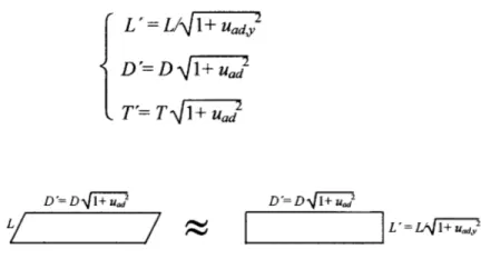
Chapter 3 extends the analysis from rainfall at a point to average rainfall intensity inside regions of various shapes. Specifically, we consider regular (square or circular) regions and highly elongated regions. The rainfall field is assumed to be multifractal and to advect with constant velocity Vad = [vad,, vady]. First we study the case when Vad = 0. A key parameter in this

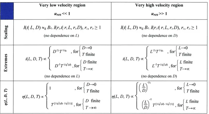
case is the ratio ures = vreslve between the "response velocity" vres = LID, where L is the maximum

linear dimension of the region, and the "evolution velocity" ve = Le/De, where Le and De are the characteristic linear dimension and characteristic duration of organized rainfall features. Then we examine the case when Vad # 0. An important parameter for advection is the ratio uad= vadve between the magnitudes of the advection velocity and the evolution velocity. For each case we study the scaling properties of the Intensity Duration Area Frequency (IDAF) curves and the Areal Reduction Factor (ARF). The results obtained are validated through simulation using multifractal cascade models. Finally we discuss the range of velocities vres, ve and vad in typical hydrologic applications.

In Chapter 4 we review observed deviations of rainfall from multifractality, in the form of dependences of the amplitude of the multiplicative fluctuations on scale. Proposed models that capture such deviations are discussed and the effects on the ARFs are studied through numerical simulation. We also study the effect of sparse spatial sampling on the estimated ARFs for different densities of the raingauge network.

Chapter 5 discusses features of the empirical Areal Reduction Factors (ARFs) proposed by the Natural Environmental Research Council (N.E.R.C.) (1975) and shows how these features can be matched by considering bounded cascade models of rainfall and sparse spatial sampling.

1 Literature review

1.1 The Areal Reduction Factor (ARF)

The Intensity Duration Frequency (IDF) curves are a commonly used tool in hydrological estimation and design. These curves give the point rainfall intensity iD,T as a function of the averaging duration D and return period T.

At a pluviometric station, iD,T is typically estimated from rainfall data by: (1) sub-dividing the historical rainfall records into intervals of duration D, (2) finding the maximum rainfall intensity averaged over D for each year in the record, and (3) ranking the yearly maxima and finding D, T such that,

1

P[I> ID,TI = (1.1)

The empirical results may be smoothed by fitting a parametric distribution to the annual maximum values or by fitting a smooth function

f(D,

iD,T =f(D, T) = (D+ ) (1.2)

where k, a, b and m are fitting parameters.

In most hydrological applications (e.g. reservoir design, flood estimation), knowledge of the point rainfall intensity iD,T _{is not sufficient. Rather, one must estimate the intensity} iAD,T averaged over area A and duration D with return period T. Clearly,

lim (iA,D,T) = D, T (1.3)

A-+O

Plots of iA,D,T produce so-called Intensity Duration Area Frequency (IDAF) curves. The IDAF curves can be estimated using an approach similar to that used for the IDF curves, with the added complication of estimating areal average intensities from point rainfall data.

In practice, it is rare to have dense networks of pluviometric stations and a more convenient way to estimate the IDAF curves is to multiply the IDF values at a point by an Areal Reduction Factor (ARF). The ARF is defined as,

Although not explicitly indicated in equation (1.4), the ARF depends also on climatic conditions, as well as the size and shape of the basin (Omolayo, 1993; Asquith and Famiglietti, 2000).

The ARF increases with decreasing area A, approaching 1 as A tends to zero. Also, the ARF increases with increasing duration D, approaching 1 as D tends to infinity. In Section 3.1, these empirical observations will be proved theoretically for a multifractal rainfall field in two spatial dimensions plus time.

Many studies have considered the effect of the return period T on the ARF with somewhat different conclusions. According to N.E.R.C. (1975), the ARF increases slightly as T decreases. Other studies (e.g. Bell, 1976; Asquith et al., 2000; De Michele et al., 2001) have found that the ARF is significantly influenced by the return period. Specifically, the latter studies find that the ARF decreases with increasing T and that dependence on A and D becomes more pronounced as

T increases.

Next we review empirical and semi-theoretical methods to estimate ARFs.

1.2 Empirical methodologies for estimating ARFs

Let iD ( = 1, ... , v) denote concurrent average rainfall intensities over D at v stations inside the

region of interest. The mean area rainfall in D, iAD, is typically estimated as a weighted average of these average point intensities,

V

A,D Iw ij& (1.5)

j=1

Frequently used weighting schemes are: 1

WI= _V- (i.e. equal weighting) (1.6)

and

A-Wi =, (1.7)

j=1

where the Aj are the Thiessen polygon areas associated with the raingauge stations inside A (Thiessen, 1911). In both schemes, the weights wj add to unity.

A number of empirical methodologies have been proposed to estimate the ARFs from rainfall records. Most of them assume that the ARF is independent of the return period (except for Bell's method, which is described later). Next we review these methodologies, as well as empirically derived ARF formulas.

1.2.1 US Weather Bureau method

After estimating the Thiessen weighting factor wi for each pluviometric station i in the basin of interest, each year j of the rainfall record is divided into intervals of a given duration D. The areal rainfall for each interval of each yearj is calculated and the interval when the areal rainfall is maximum is found. Finally, the ARF (assumed independent of the return period ) for duration D is estimated as

n V f V

ARFus = vj I wi AP,1 ZPi,Q (1.8)

j=l i=1 j=

where Pi, is the annual maximum point rainfall in D at station i in yearj, P',1 is the point rainfall in D at station i on the day when the annual maximum areal rainfall occurs in year j, v is the number of stations in the basin and n is the length of the data record in years.

The method uses different weighting schemes: Thiessen weighting for P,1 in the numerator

and equal weighting for P, in the denominator.

Based on the assumptions that the ARFs are independent of the return period T, and on the geometry of the basin, Leclerc and Schaake (1972) used equation (1.8) to derive the following empirical relation for ARF(A, D):

ARF(A, D)= I- exp(-1.1 D~0.2 )+ exp(-1.1 D - - 2.59x10' A) (1.9)

where A is in [KM2_{] and D is in [hours]. Weather Bureau (TP-29) specifies ARF for areas up to}

I JMMMW '_ - - 0.9 0.85 0.8 4~---LI. 0.75 0.7 -A_ CC _______________________ D = 1 ho ur M M D = 3 ho u rs - - - D= 6 hours D=24 hours 0.55 0.001 0.01 0.1 1 10 100 1000 10000 Area (kmA2)

Figure 1.1: Leclerc and Schaake ARF curves for durations of 1, 3, 6, and 24 hours and areas up to 1 100 Km2

.

One can observe In Figure 1.1 that for A small (say A < 5 KM2) ARF is nearly constant and equal to 1. This behavior of the ARF is in agreement with the fact that for A = 0 the IDAF curves reduce to the IDF curves and thus ARF = 1. For intermediate values of A (say 10 Km2 <A < 100 KM2) the ARF is approximately a power function of AID, whereas for A large (say A > 100 Km2) the ARF depends only on D. This behavior of the ARF for large A is not supported by other studies (see for example N.E.R.C.'s diagram, Section 1.2.2), and it is probably associated with data limitations for large areas.

1.2.2 N.E.R.C. method

Assuming independence of T and using equal weighting, N.E.R.C. (1975) calculates the ARF as

I

ARFNERC -- _nvj= Z' _i= ,E (1.10)

N.E.R.C. (1975) used equation (1.10) to estimate the ARFs for thirteen basins in the United

2

Kingdom with areas ranging from 10 to 18 000 Km . Averaging durations ranged from 2 minutes to 25 days. N.E.R.C. then smoothed and interpolated the empirical results to obtain the diagram in Figure 1.2 (for a more detailed review of the data and the fitting procedure see

10000 -r / / / vol / ,/ / 2 / "~ -~ / / *~1'~~ / / (45;, I ,~ ~ / / voi / / ~ 4~'] 1000 / ______ /

I:

1/

LI

I

2I ~I'~' .,x;;4j14j4:§4

I

1

/

Figure 1.2: ARFs for durations D from 15 minutes to 8 days and areas A from 10 to 10 000 Km2

. Reproduced from

N.E.R.C. (1975) Flood Studies Report, Vol. II, p. 40.

According to N.E.R.C. (1975), these ARFs correspond to rainfall events with return period

T= 2-3 years.

A general fit to the UK N.E.R.C. (1975) data shows that the ARF is approximately constant for D oc A0'7. However, the N.E.R.C. iso-ARF curves indicate a variable slope, with D oc A0

.5 for large A and small D, and larger A exponents for lower areas or larger D (for a more detailed analysis see Section 5.2).

Based on these N.E.R.C. curves, Koutsoyiannis (1997) derived an analytical expression for the ARF,

0.048 A 0.36 -0.01 ln(A)

ARF= I - o.35 > 0.25 (1.11)

where A is in Km2 and D is in hours. This expression is shown graphically in Figure 1.3.

250

~n

94R

n nfin

U-0.001 0.01 0.1 1 10 100 1000 10000 100000

A (kmA2)

Figure 1.3: Koutsoyiannis ARF curves for durations of 1, 3, 6, and 24 hours and areas up to 30 000 Km2. 1.2.3 Bell's method

This method takes into account the variation of the ARF with return period T. Suppose that the rainfall records cover a period of a year. The annual maximum areal and point rainfall series are both ranked in descending order. The ARF with given rank r and thus return period T (e.g.

n-i

T_= _r ) is estimated as the ratio of the areal rainfall of rank r to the sum of the weighted (e.g.

Thiessen weights wi, i =1, 2, .. .,v) point rainfalls of the same rank,

ARFT)Bell= w ,r WiPi,r (1.12)

1~ Ii=1

If the ARF is independent of the return period, then

ARFBell =

X-

r=1

If moreover one uses equal weighting (i.e. wi = 1/v), then equation (1.13) reduces to the N.E.R.C. method (equation (1.10)).

1.3 Semi-theoretical methodologies for estimating ARFs

Several studies have tried to derive the ARF (or IDF or IDAF) curves using probabilistic models of space-time rainfall. An early attempt in this direction was made by Roche (1966) who

0.7 0.6 0.6 0.3 D=1 hour D=3 hours 0.2 - - - D= 6 hours - D=24 hours 0.1

developed a theoretical approach to point and areal rainfall based on the correlation structure of intense storms.

Rodriguez-Iturbe and Mejia (1974) extended Roche's (1966) approach by assuming that the rainfall field is a zero mean stationary Gaussian process. Averaging over the catchment area A results in a variance reduction factor i2 given by

K2=Elp(||x2- xli)] (1.14)

where E[p] is the expected spatial correlation coefficient between two points xi and x2

independently and uniformly distributed inside the catchment area, and

||

||

K2=

f

0

where R is the random distance between x, and x₂, and gR(r) is the Probability Density Function (PDF) of R. Notice that K2 _{is a function of the spatial correlation structure of rainfall and the size}

and shape of the catchment. Rodriguez-Iturbe and Mejia (1974) argued that K, the square root of these variance reduction factor, could be interpreted as the ARF (i.e. ARF= K).

In the method of Rodriguez-Iturbe and Mejia (1974), the mean of the averaged rainfall intensity does not change with the catchment area. However, this is a property of the stationary parent process not the extreme value process that is of interest for ARF determination. Therefore, the theoretical validity of the ARFs calculated by this method is limited.

Another important limitation is that, the method does not account for the effect of duration D on the ARFs. It is assumed that this information is included in the spatial autocorrelation function p(r). Thus, the effect of the duration D on the ARF is not clear.

A different approach, based on crossing properties of random fields, was proposed by Bacchi and Ranzi (1996). This approach assumes stationarity of the rainfall field and homogeneity of the crossings in space and derives a complicated expression for the ARF that incorporates a large number of fitting parameters that have to be inferred from data.

Bacchi and Ranzi (1996) argue that the ARF increases with decreasing A and increasing D. Furthermore, they find a small decrease of the ARF with increasing T.

Properties of extremes of random functions were used also by Sivapalan and B16schl (1998). The starting point of their approach is to derive the parent distribution of the catchment average

rainfall intensity from that of point rainfall intensity assuming stationarity of the rainfall field in space and time. Sivapalan and B16schl (1998) start from the assumption that the parent distribution of the point rainfall intensity ip is of the Exponential type,

A ip) exp (1.16)

with mean = , and variance (oP)2 2_{.They further assume that the spatial autocorrelation}

function of the rainfall field is isotropic exponential,

pp(r)= exp (1.17)

where r is separating distance and A is the spatial correlation length, defined as

=f pp(r) dr (1.18)

0

The areal rainfall parent process iA is assumed in approximation to have a Gamma distribution,

kAexpC-fAiA)= PA -(kA) (1.19)

with mean pA = kA

PA

kA (PA)2. The parameters of the distributions in equations (1.16) and (1.18) are related as

kA PA = 3pk (1.20)

kA (A) 2 )2 _(1.21)

where K2 is a variance reduction factor defined in the same way as in Rodriguez-Iturbe and Mejia (1974); see equation (1.14). The parameters

p,,

and point rainfall intensities with the same duration and return period, is given by

K2

ARF(2 , D, T)=( T (1.22)

b(D) c(D) -i nln(T-)

A __2

ARF(K 7)= 72) (1.23)

which indicates that the ARF depends solely on the catchment area A and the spatial correlation structure of the rainfall field, which is expressed through K2. The method does not directly

account for the duration D of the rainfall event, and it is argued that this piece of information is included in the spatial correlation structure of the field. The calculated ARFs, increase with decreasing A and increasing D, and are highly dependent on both the return period T and the spatial correlation function pp(r) of the point rainfall process.

Also the work of Asquith and Famiglietti (2000) can be considered to belong to this class of stochastic methods. Their methodology is based on two assumptions: (1) the largest potential volume of a storm occurs when the storm is centered over the centroid of the basin, and (2) the cross-correlation of concurrent precipitation at two non-centroid locations is insignificant. Although the former assumption seems plausible, the latter is not. This is so because the spatial correlation structure of rainfall is an important parameter that affects the ARF; see above.

The derivation of the ARF is performed through a function ST(r) defined as the expected value of the ratio between the rainfall depth at some location a distance r from the centroid of the design storm and the depth of the annual maximum with return period T at the same location. Si(r) depends on return period T and describes the spatial structure of a storm radiating away from the centroid of the basin.

Asquith and Famiglietti (2000) estimate the ARF as the ratio between the T year rainfall depth over a catchment area A and the point rainfall depth ZT with return period T at the centroid of the storm, i.e.

ZT f Sr) dx dy f S(r) dx dy

ARF(A, ) = - (1.24)

The method does not directly account for the duration D of the rainfall event, and thus the influence of D on the estimated ARFs is not clear. The approach produces ARFs that are significantly influenced by the return period T. Specifically, for longer return periods T the estimated ARFs decay faster with increasing A.

the spatial dependence of point rainfall without special focus on extremes (the above mentioned approaches are of this type) and those that focus on extremes and pay less attention to spatial dependence. Coles and Tawn (1996) propose a method of the latter type.

A third class of methods exploits the scaling properties of space-time rainfall. Scaling ideas for temporal rainfall have been used by Hubert et al. (1993), Benjoudi et al. (1999) and Veneziano and Furcolo (2002a) to derive scaling properties of the IDF curves. The latter two approaches will be reviewed in detail in Section 2.3.

Also De Michele et al. (2001) pursued a scaling approach to explain the ARF and the IDAF curves. Defining I(D, A) as the maximum annual value of the mean rainfall intensity for duration D and area A, De Michele et al. (2001) argue that I(D, A) could have either self similar or multifractal scaling properties with D and A. Then they focus exclusively on the self similar property stating that I(D, A) must have the form,

I(D, A-ao) = Da g(A ao) (1.25)

where ao is the collection area of a raingauge, g is some random function and a, b and c are

scaling exponents. By reasoning on the limiting behavior of I(D, A) as A -+ 0 and A or D -> 00,

De Michele et al. (200 1) conclude that g must have the form,

J(A-ao) = (A -ao) -f(

D1 = ai 1 +> DC (1.26)

where ai is the random intensity in ao for T = 1, and co and 8 are constants. The argument by which equation (1.26) is derived is not clear. The constants a, b, c, co and / are determined from data (relations among these constants allow one to reduce them to 4 independent parameters).

The approach of De Michele et al. (2001) makes direct assumptions on the scaling of annual maximum rainfall, without deriving such properties from the scaling of the rainfall field itself.

This "shortcut" makes it difficult to choose on conceptual grounds between self similarity and

multifractality of the annual extremes and also makes it impossible to link the scaling exponents of the ARF and IDAF curves to properties of the rainfall field (e.g. stratiform vs. convective, summer vs. winter precipitation), determine the effect of return period T on the ARF, and characterize the distribution of the random variable ai in equation (1.26). All these properties

and parameters have to be inferred from data. Moreover, the way in which the area of the raingauge collector is treated in equations (1.25) and (1.26) destroys scaling.

From application to a region near Milan (8 years of data, 16 stations covering an area of about 300 kM2_{), De Michele et al. find dynamic scaling with D proportional to A, whereas a}

general fit to the N.E.R.C. (1975) data gives D oc 0-7; see Section 1.2.2.

In a recent study, Castro et al. (2004) developed a multiftractal approach to explain how the IDAF curves scale with A, D and T. Castro et al. (2004) assumed anisotropy of rainfall in space and time with D proportional to AZ/2_{, where z is a scaling coefficient estimated from data. Using}

a large-deviations property of multifractal fields, Castro et al. (2004) find that

iAD,To D -'A-z/2 T 6 (1.27)

where 3 is a positive constant independent of T, which is estimated from data. Castro et al. (2004) do not discuss the exact derivation of equation (1.27). They also argue that 3 is given by

= I-c(y) (1.28)

where c(y) is the co-dimension function of rainfall when approached as a ID multifractal process in time. Although not explicitly stated, the analysis of Castro et al. (2004) is valid only for large values of T. This is so because the ratio 1-c(y) becomes a constant independent of y, and thus T, only for y y*, i.e.

-Y _{, y > Y}

(1.29)

1-c(y) q*

where y* is the highest singularity order for which the moment scaling function of the temporal rainfall process is finite, and q* is the associated moment order greater than 1; see Section 2.2.2. From an application to a rainfall event in Mexico, Castro et al. (2004) find 3 = 1.227 and

z = 1.161. Since z ~ 1 one can conclude that rainfall is in approximation isotropically multifractal in space and time. However, one should be cautioned that 3 = _{1.227 corresponds to}

f-y

I-c(y) ~ 0.82. Thus y < y and hence 3 is not a constant independent of T as argued by Castro et

In this thesis, we study the behavior of Areal Reduction Factors (ARFs) under multifractality, determine the effects of deviations from exact multifractality, and quantify the bias from the estimation of ARF from sparse spatial data. We also study the effect of rainfall advection on the ARF. The effect of advection depends on the shape, size and response time of the basin. Finally we discuss observed features of empirical Areal Reduction Factors (ARFs) and show how these features can be explained using scaling properties of rainfall, deviations from perfect scaling, and biases from sparse spatial sampling.

2 Extremes of multifractal rainfall in time

In hydrological risk analysis and design, knowledge of the probability of rainfall extremes is essential. However, available data rarely allow one to directly estimate rainfall intensities over the range of areas, durations and return periods of practical interest. One way to make the inference of rainfall extremes more robust is to use model predictions. Multifractal models provide a good representation of space-time rainfall fields (Lovejoy and Schertzer, 1995; Gupta and Waymire, 1993; Deidda, 2000). Therefore, one can use the theory of multifractality as a framework to elucidate the behaviour of empirical rainfall extremes and extend the results beyond the empirical range of A, D and T. For example, Bendjoudi et al. (1999) and Veneziano

and Furcolo (2002a) used multifractal rainfall models to determine certain scaling properties of the Intensity Duration Frequency (IDF) curves.

We start in Section 2.1 by reviewing a result in large deviation theory known as Cramer's Theorem. This theorem forms the basis of the analysis that follows.

In Section 2.2, we review certain extreme properties of discrete multifractal cascades, which are the simplest models displaying multifractal behaviour (Gupta and Waymire, 1993). First we describe how a multiplicative cascade is generated and define the concepts of bare and dressed measure densities. Then we derive properties of extremes of bare and dressed densities through linkage to and an extension of Cramer's Theorem.

Section 2.3 uses the previous results on cascades to derive properties of the IDF curves. In particular, we review the approaches by Bendjoudi et al. (1999) and Veneziano and Furcolo (2002a). Benjoudi et al. (1999) focus on the limiting case when D is finite and T-+oc, while Veneziano and Furcolo (2002a) derive the scaling properties of the IDF curves for: (1) D-+0 and T finite and (2) D finite and T-+oc. For the second case with D finite and T-+oc the results of Veneziano and Furcolo (2002a) are the same as those of Bendjoudi et al. (1999).

Conclusions and comments on the foresaid approaches are summarized in Section 2.4.

2.1 Cramer's Theorem for sums of independent random variables

Cramer's Theorem is a fundamental result in large deviation theory. The theorem deals with a property of extremes of sums or averages of independent and identically distributed variables. The reason why normal theory does not apply is that the extremes of interest move farther and

farther into the tail of the distribution as the number of added or averaged variables increases. These extremes are in a region of the distribution that has not yet converged to a normal shape. We review in detail the derivation of the theorem, because this result is essential to all the developments that follow in this chapter. For additional information on Cramer's Theorem and related results the reader is referred to Den Hollander (2000), Dembo and Zeitouni (1993) and

Stroock (1994).

Let Sn = 1(X 1 + .. +. Xn) be the average of n independent copies of a random variable X with

Cumulative Distribution Function (CDF) F. Assume that X is unbounded and that the moment generating function,

M(q) = E[e]

f

-OC

is finite for all q ? 0. Using the fact that the X are independent and identically distributed, one obtains

n

E[ensn]=

H

1= 1

Next we use a result in probability theory called Markov's inequality (Papoulis, 1990, p. 131). This inequality states that, for any non negative random variable U and any positive constant 6,

1

P[U> 6E[U]] 3 (2.3)

Application to U= eqsn and use of equation (2.2) gives

1

P[enqs" > 5 M(q)"] ,>0 6 and q ? 0 (2.4)

or, solving for Sn

1

Sn qln(6)+ 1 :, 6>0 and q :0 3n>M(q) (2.5)

1 1

If we define y =- ln(3) + - In{M(q)}, then 3 = M(q)-" e"'q and equation (2.5) becomes

nq q

where K(q) = ln(M(q)). By minimizing the right hand side of equation (2.6) with respect to q we

obtain

P[S, > y] exp(-n max{qy -K(q)}) (2.7)

q O

We now introduce the Legendre transform of K(q) as the function c(t) given by

c(t) = maxlqt - K(q)} , -OC < t < Oc (2.8) q

Using c(t) and taking logs, equation (2.7) becomes,

ln(P[Sn y] )

n -c(y) (2.9)

For y > E[X] one can show (for details, see Stroock 1994, p. 30) that, in the limit as n -+ oc, the

inequality in equation (2.9) becomes an equality, giving

lim = -c(y) (2.10)

This result is known as Cramer's Theorem (Cramer, 1938).

The condition M(q) < oc for all q > 0 is not necessary for equation (2.10) to hold. For example, equation (2.10) is known to hold also for M(q) finite in an infinitesimal right and left neighborhood of zero (Dembo and Zeitouni, 1993, section 2.2.1). Under the latter condition and for X continuous, equations (2.9) and (2.10) can be refined (Cramer, 1938, p. 5-23) as

P[Sn > y] = g(y, n) enc(Y)

g(y, n) = (27n C "(Y)) (1+0(1)) (2.11)

where the ' and ' signs denote the first and second derivative respectively, and o(1) is a term that vanishes as n goes to infinity. Similar asymptotic results have been derived by Bahadur and Ranga Rao (1960) for X not continuous. Equation (2.11) is used next to derive properties of multifractal extremes.

2.2 Extremes of bare and dressed multifractal cascades

There is a direct analogy between certain multifractal extremes and the large deviation behavior of sums of independent identically distributed random variables.

Consider an isotropic multiplicative cascade. The cascade construction starts at level 0 as a uniform unit measure in the d-dimensional cube Sd. The multiplicity of the cascade is m, where

m is an integer larger than one. This means that, after n cascade levels, Sd is divided into m nd

cubic tiles Tj1 (i = 1, ... , m"d) with linear size m-. The measure density inside T., is obtained by

multiplying the measure density of the parent tile at level n-I by a random variable Y,i with unit mean value. Although in general the random variables Y; may be dependent both within and among cascade levels, here we consider only the case when the Y,,, are independent copies of a random variable Y, called the generator of the cascade.

Let cmn be the average measure density of the cascade inside a cube of linear size m-, or at resolution m". One may distinguish between two types of such average densities: the bare measure density Emw,b and the dressed measure density cm,,d. The difference between bare and dressed densities is that the former does not include fluctuations at scales smaller than m-". Thus,

Emfl,b is the measure density within a tile T.1 when the multiplicative cascade construction is

terminated at level n. By contrast, the dressed measure density is the average density in T., for the completely developed cascade. The two measure densities are given by

n

Em-,b i

:

I=

=m~ Cmn,b Z

where Yi, Y2, ... , Y,, are n independent copies of Y and Z is the so-called dressingfactor, which is independent Of Emn,b and has the same distribution as cl,d, the dressed measure in Sd.

Next we derive extreme value properties of the bare and dressed measure densities from Cramer's Theorem.

2.2.1 Extremes of bare densities

Let X = logm(Y), so that

n n

logm(em,b)= $ logm(If)= (Y X= nl Sn (2.13)

i=1 i=1

where Sn = (X₁ + .. X). n.+ In multifractal analysis one often characterizes the distribution of Y

Kb(q)= logm E[] ln(m) (2.14)

and its associated Legendre transform

cb(y)=max{qx - K(q)} = ,-oc< x < C (2.15)

q>O ln(m) '

The function Kb(q) is the bare moments scalingfunction of the cascade. In fact, for any q for

which E[Y] exists, equations (2.12) and (2.14) give

E[(Em-,b)q]= E[n]= InK(q) (2.16)

Using equation (2.13) and the results on Sn, in equations (2.10) and (2.11) one obtains the following extreme properties of bare multifractal measures:

1

lim I log(P[mn,b > M"9) = -Cb(y) , y > E[log(Y)] (2.17)

and

P[Em,b mn = g(y, n) m-"ncb()

g(y, n)= (2nn ln(m) Cb(y) (2.18)

Since n ln(m) = ln(mn), the function g(y, n) varies slowly with the resolution of the cascade m". One often states equation (2.18) as

P[Emn,b M"'] ~ M -"cbO) (2.19)

where ~ denotes equality up to a factor that varies slowly with the resolution m". 2.2.2 Extremes of dressed densities

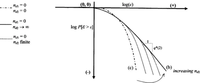
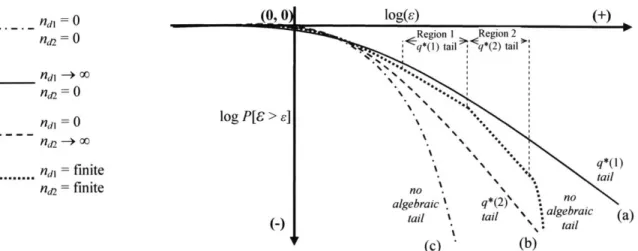
The main novelty when dealing with dressed densities Emn,d is that the moments Of Cmwd above some finite order q* may diverge. This critical order q* is given by the conditions q* >1 and Kb(q*) = d (q* - 1) (Kahane and Peyriere, 1976; Schertzer and Lovejoy , 1987), where d is the Euclidean space dimension. Therefore, q* is a function of d. When needed for clarity we shall indicate this dependence by using the notation q* = q*(d). Similarly to bare densities, the moments of the dressed densities have a power law dependence on the resolution m". In fact,

where the dressed moment scaling function Ka(q) is given by

{K(q) , q < q'

Kd(q) =

{

Veneziano (2002) showed that the dressed densities Em,,d satisfy a large-deviation relationship similar to equation (2.18),

P[Cmn ,d> m"1 = h(y, n) m ncly) (2.22)

where cd(y) is the Legendre transform of Kd(q),

ca(y)= max{qy - K(q)} = {. . (2.23)

q q y + d(q*- 1), y > y

d is the Euclidean space dimension, y* = _{Kb'(q*) and h(y, n) is a function that varies slowly with} the resolution m"; see Veneziano (2002) for details on the form of the function h. In analogy with equation (2.19), one can write

P[Cmn,d Mi ] m-ncjy) (2.24)

For q* finite, the moments of 6_{mn,d above order q* diverge and the distribution of}

Emn,d must have

an algebraic upper tail of the type

lim P[Cmn,d s] ~ s~q* (2.25)

S--Jc2

This tail behavior of the dressed densities is due to the algebraic tail of the dressing factor Z.

2.3 Scaling properties of the intensity duration frequency curves

This section reviews past work on the scaling properties of the IDF curves under the assumption that rainfall is a stationary multifractal process. Two approaches are presented, one by Bendjoudi et al. (1999) and the other by Veneziano and Furcolo (2002a), which in different ways utilize the extremal properties of multifractal cascades given in Section 2.2.

First, we introduce some notation. Let ID be the average rainfall intensity in a time period of

duration D. We assume that ID is stationary multifractal with random generator A,. This means

that

ID d Ar IrD (2.26)

Also define T(D, i) to be the return period of the event ID> L- The return period T(D, i) can be expressed in different ways. A standard definition is

Ti(D, i)= _P[Ima,D 1 _{> i} (2.27)

where Imax,D is the maximum of ID over a unit time period (e.g. one year). Equation (2.27), with a unit time period of one year, is appropriate when, as in rainfall, the phenomenon of interest has seasonal variations. In the context of a stationary model an often more convenient definition is,

T2(D, i) P D (2.28)

which is the reciprocal of the expected number of D intervals in a uniform partition of the unit time interval when ID> L. This second definition of return period is the one used by Bendjoudi et

al. (1999) and Veneziano and Furcolo (2002a) and is the one used in the rest of this chapter.

2.3.1 Bendjoudi et al. approach

Although not explicitly stated, the analysis of Bendjoudi et al. (1999) aims at deriving the scaling properties of the IDF curves for large T and small D.

Since rainfall at a point is a multifractal process in time, the Euclidean dimension of the observation space is d = 1. Bendjoudi et al. (1999) do not use this condition and rather consider

d as a parameter to be determined. As in equation (2.23), they write the co-dimension function

of the rainfall process for y > y* as

cd(y)= q* y - d(q*- 1) (2.29)

where q* depends on d. Then, using equation (2.22) with em.,d = ID and m" =Dax/D, Bendjoudi et

al. (1999) write

C~waxDmax-q* y + d(q* -1)

ID D

.

where 7(y, Dmax/D) = _{h(y, logm(Dmx/D)). Introducing the condition I{ID> (D ] which} comes from the definition of the return period in equation (2.28), and replacing (Dax/D)y with

D= h(y, Dma/D) i(D, T)-q* (Dmjd(q* - 1) (2.31)

Next, Bendjoudi et al. (1999) argue that the function 1_{(y, D,,a/D) may be considered constant.}

Thus,

i(D, T) cc D -(d(q* -1) + I)/q* T l/q* (.2

If one now sets d = 1 (the physical dimension of the observation space for point rainfall) one obtains

i(D, T) oc D~1 T lq*() (2.33)

where q*(1) is q* for d = 1. This implies that the yearly maxima Imax,D scale with D in the self similar way

Imax,D d r Imax,rD (2.34)

2.3.2 Veneziano and Furcolo approach

First, Veneziano and Furcolo (2002a) extend equation (2.22) to obtain an expression for P[Cmn,d > a m"], where a is a given positive constant.

Writing a rJ= r + IOgra, one may use equation (2.22) to obtain

P[Er,d > a r] = P[Er,d r Y' +Iogra] = (y + logr a, r) r-cy + Iogra) (2.35)

where /i(y, r) = h(y, log,, r). Using Taylor series expansion, one can approximate the function

Cd(y + logr a) for large r as

Cd(y + logr a),& cd(y) + cd'(y) logr a (2.36)

Then equation (2.35) becomes

P[Er,d > a r] ~ /(y + log, a, r) a-c'() r-cy) (2.37) Using equation (2.23) one can prove that cd'(y) in equation (2.37) is given by

{q(y) , y -- y*

Cd'(Y) = > * (2.38)

Veneziano and Furcolo (2002a) use equations (2.35) and (2.37) to derive results on the IDF curves, as summarized below.

If rainfall intensity has mean value p = E[ID], then ID has the unit-mean cascade representation,

ID I CDma/D,d (2.39)

where D is the resolution. Thus, using equation (2.35),

P [ID pa1 1 D

= y+ logDwa/D (a), D 7 (D) d( a) (2.40)

D

Recalling from equation (2.28) that i(T, D) satisfies P[ID > i] , one wants to find a and y such DT

as the right hand side of equation (2.40) equals D, i.e.

(

D

when log~a/D (a) is infinitesimal. This condition attains for any finite T and D -~ oc. This

means that logDm,/D (a) -- 0. Hence using equation (2.36), equation (2.41) becomes,

hy, 2"a-( D -cfy) = (2.42)

The property that h(y, r) is slow varying in r implies that, for any given D1 and D2, . h(y, Dma /Di)

D -- oc h(y, Dmax/D 2) (2.43) i.e. for large Dmax/D the function h y' D

,)

y = yi and a oc ( (2.44)

where yi is such that cd(y1) = 1 and q, = q(yi) is the associated moment order. Since yj < y*, for the derivation of equation (2.44) we have used cAdO1) = q(yi) in equation (2.38). Also, it is a

the dimension of the observation space d. Equations (2.42) and (2.44) imply the following scaling relationship of i(D, T) with D and T.

i(D, T-) oc D-" T /N, (2.45)

Equation (2.45) gives the scaling properties of the IDF values for T finite and D-+O. An interpretation of equation (2.45) is that for D small the annual maxima Iax,D satisfy the self similarity condition,

Imax,D d r" Imax,rD (2.46)

However, notice that equation (2.45) was derived using the definition of return period in equation (2.28) not (2.27) and hence without reference to the definition of the annual maxima. Therefore the interpretation in equation (2.46) is not strictly correct.

The second case considered by Veneziano and Furcolo (2002a) is when y + logD/D (a) > y*, which occurs for large T and relatively small Dmax/D ratios. Given that y + logD.a/D (a) > y* and using equation (2.29) for d= 1 (Euclidean dimension of the observation space), the co-dimension function has the form

cd(y + logD/D a) = (y + logD/D a) q*(l) -(q*(l) - 1) (2.47)

and equation (2.41) becomes,

y + logDw.a/D (a), a*()*() y +q*()- = (2.48)

if /(y + logD/D (a), does not vary much with either D,Ix/D or a, then equation (2.48) is satisfied for

y = 1 and a oc - (2.49)

Therefore, for very large T the IDF values scale as

i(D, ) oc D71 T1/q*(') (2.50)

This is the same as the relation derived by Bendjoudi et al. (1999); see equation (2.33). From equation (2.50) one concludes that, in the extreme upper tail, the annual maxima Imax,D satisfy the self-similarity condition

Imax,D d r Imax,rD

The scaling properties of the IDF curves for the above limiting cases have been validated numerically by Veneziano and Furcolo (2002a).

2.4 Conclusions and comments

The analysis of Bendjoudi et al. (1999) aims at deriving the parameters q* and d from IDF curves estimated empirically from rainfall records. Although not explicitly stated, their analysis

is valid for large T and small D. If the empirical IDF curves have the form,

i(D, T) oc D'Y# (2.52)

then Bendjoudi et al. (1999) find q* and d by equating the scaling exponents in equations (2.32) and (2.52). For example, using an empirical formula of the type in equation (2.52) obtained by Farthouat (1962) for the Bordeaux area, Bendjoudi et al. (1999) find q* = 2.78 and d= 0.64. However one should be cautioned that q* is a function of d, and independent estimation of these two quantities from rainfall data is not mathematically correct. Moreover, values of d (dimension of the observation space) other than 1 seems to make little physical sense. The likely reason why values of d smaller than 1 are obtained, is that the empirical IDF curves where derived for return periods T 20 years and in this range the theoretical analysis of Bendjoudi et

al. (1999) does not apply.

The analysis of Veneziano and Furcolo (2002a) is more complete. It derives the scaling properties of the IDF curves for two liming cases: (1) D-+0 and T finite and (2) D finite and

T-+oc. For D-+0 and T finite, the theoretical dependence of i(D, ) on D is of the type D-' with

0 < yj < 1. This corresponds better to the empirical results of Farthouat (1962) and indeed to the value of the exponent of the empirical IDF functions, which is typically in the range [-0.7,

-0.6]. For the second case with D finite and T-+oc, the results of Veneziano and Furcolo (2002a) are the same as those of Bendjoudi et al. (1999) for Euclidean dimension of the observation space d= 1.

3 Extremes of multifractal rainfall in time and space

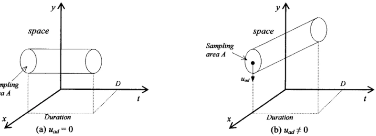
In Chapter 2 we analyzed the behavior of rainfall extremes when rainfall is observed at a point on the geographical plane. Here we extend the analysis to the average rainfall intensity inside regions of various shapes with maximum linear size L. Specifically, we consider regular (square or circular) regions and highly elongated regions in which the narrowest dimension is much smaller than L. On the geographical plane (x, y) the maximum elongation is assumed to be in the y direction; see Figure 3.1.

L

Regular Highly

shape elongated

shape

x

Figure 3.1: Schematic representation of regular and highly elongated regions.

In a Lagrangian reference the rainfall field in (x, y, t) space is assumed multifractal. The

field advects with constant velocity Vad = [Vad,x, Vady] ', where the superscript T denotes the

transpose of a vector. We consider first the case when Vad = 0 and then examine the effect of Vad

# 0. For each case we study the scaling properties of the Intensity Duration Area Frequency (IDAF) curves and the Areal Reduction Factor (ARF). These properties further depend on the shape of the region.

The chapter is organized as follows. Section 3.1 derives properties of the IDAF curves for the case Vad = 0. This is mainly an extension of the work of Veneziano and Furcolo (2002a) on

the Intensity Duration Frequency (IDF) curves for the case of point rainfall. Using these results, we obtain the scaling properties of the IDAF curves and the ARFs with the size of the region L, the period of aggregation D and the return period T. We do so for three limiting geometries of the rainfall collecting region: a regular 2D region (a square or a disc), a line segment and a point. A key parameter in this analysis is the ratio ures = vreslve between the "response velocity" vres = LID and the "evolution velocity" ve = Le/De, where Le and De are the characteristic linear