Areal Representation Issues in Using Census Data for Urban Research:
A Comparative Analysis of Japanese and U.S. Formats
by
Yoshimasa Ito
B.S., Civil EngineeringMassachusetts Institute of Technology, 1993
SUBMITTED TO THE DEPARTMENT OF URBAN STUDIES AND PLANNING IN
PARTIAL FULFILLMENT OF THE REQUIREMENTS FOR THE DEGREE OF MASTER IN CITY PLANNING
AT THE
MASSACHUSETTS INSTITUTE OF TECHNOLOGY JUNE 1996
@ 1996 Yoshimasa Ito. All rights reserved.
The author hereby grants to MIT permission to reproduce and to distribute publicly paper and electronic copies of this thesis document in whole or in part.
Signature of Author:
Department of Urban Studies and Planning April 17, 1996
Certified by:
Accepted by
Qing Shen Assistant Professor of Urban Studies and Planning
Y
7hesis Supervisor:7
;'ASSACHUS1rTS pSimurs Asso ate Professor OF TECHNOLOGY
J. Mark Schuster
of Urban Studies and Planning Chairman, MCP Committee
JUL 0
21996
Rfen
Areal Representation Issues in Using Census Data for Urban Research:
A Comparative Analysis of Japanese and U.S. Formats
by
Yoshimasa Ito
Submitted to the Department of Urban Studies and Planning on April 17, 1996 in partial fulfillment of the requirements for the Degree of Master in City Planning
ABSTRACT
Spatial data are methodical representations of physical reality. Because there are many possible representations for any reality, spatial data users will encounter different representations. Therefore, it is important that spatial data users develop abilities to explore the various strengths and limitations that are associated with the formats of the spatial data that they use for research.
This thesis explores the effects of different census data formats on spatial analyses within the context of urban studies and planning, through a comparative analysis of the Japanese and United States census data. These data formats represent extremely different methods of representing spatial reality. The Japanese "mesh" data format is an example of 'raster'
representation, while the U.S. approach is a 'vector' representation of geographic areas. Four urban-related problems that utilize census data are examined. Each problem contains elements that expose the characteristics of the census data formats being applied, while representing a broad category of urban problems.
The methodology for this analysis is three-tiered. First, a review of literature that discusses the general issues related to spatial data use, as well as issues that are specific to the urban-related problems, is conducted. Then, the methodologies for defining the geographic entities in each census data format are described. Third, the issues and complexities associated with the application of census data to these urban problems, as well as possible procedures or tools that may facilitate the analyses, are explored.
The findings indicate that the degrees of suitability for utilizing these census data formats depend on the particular needs of both the urban problems and their broad categories. Generally, the strength of the U.S. census format is evident in enumeration, analyses of areas pre-defined by political or physical boundaries, and urban analyses where high spatial resolution is desired. The Japanese mesh squares facilitate temporal analyses of larger regions, definition of the analysis area by some urban models, and analyses where areal unit consistency is desired. Land-use information in the form of maps or remote sensing data is described as a potential tool for facilitating some of the analyses.
Thesis Supervisor: Qing Shen
Acknowledgments
Thank you, Professors Qing Shen and Joe Ferreira, for allowing me to selfishly complete my thesis under a very unusual time constraint, and for enabling me to start developing some ideas about spatial data and their roles in urban studies and planning. It is hard to believe that it's been almost five years since I started hanging around at the Computer Resources Laboratory as a UROPer.
Professor Atsuyuki Okabe of the Faculty of Urban Engineering, University of Tokyo, offered me valuable advice and readings when I began to examine the Japanese "mesh" census data format. During my ten-month stay as a research student at the University, I
also received valuable help from Professor Yasushi Asami, Dr. Yukio Sadahiro, Keiichi Okunuki and Yutaka Gotoh, all of Okabe/Asami Laboratory.
My grandfather passed away due to a sudden illness, as this project was getting under
way. Although physical distance kept us from seeing each other frequently, he offered me much needed support and encouragement during the last several years.
Table of Contents
Abstract
... 2
Acknowledgments
... 3
Chapter 1:
Introduction
... 6
1.1 Statement of the Problem
1.2 Research Methodology
Chapter 2:
Literature Review
... 11
2.1 About the Data 2.2 Use of Spatial Data
2.3 The Proposed Urban Studies and Planning Problems
2.4 Discussion
Chapter 3:
The Census Data Formats Examined
... 19
3.1 Japanese Census Data Format
3.1.1 Early Versions of Japanese Census Data 3.1.2 Creation of "Mesh" Census Data in Japan 3.1.3 Basic Processing of Mesh Data
3.2 U.S. Census Data Format
3.3 Comparing Inherent Characteristics of the Two Representations
Chapter 4:
Counting of Populations Using Census Data
... 37
4.1 Methods for Counting People
4.2 Relating Census Data and Spatial Representation 4.2.1 Assigning Attribute Data to Japanese Census Mesh Squares 4.2.2 Assigning Attribute Data to U.S. Census Geographic Entities 4.3 Counts of Specified Regions Using Census Data
4.3.1 Enumeration with U.S. Census Data 4.3.2 Enumeration with Japanese Census Data 4.4 Discussion
Chapter 5:
Measuring Population and Employment
Changes Over Time
...
48
5.1 Non-static Geographic Entities Over Time
5.2 Forecasting and Estimations for Non-census Years 5.3 Meaningful Areal Units for Urban Research
5.4 (Mis) representation Using Maps
5.5 Discussion
Chapter 6:
Inter-city Transit Demand Models and Census Data
... 66
6.1 Description of Example: Suburban Rail Station 6.2 Definition of Gravity Model
6.3 Critique of Model and Mesh Representation 6.3.1 Spatial Resolution and Population Homogeneity
6.4 Discussion
Chapter 7:
Evaluating Usage of Local Transit Stops
... 76
7.1 Different Types of Ridership Forecast Models 7.2 The Period Route Segment Model
7.3 Description of Example: Hakodate, Japan
7.4 Extracting of Data
7.5 Critique of Model and Census Formats 7.6 Discussion
Chapter 8:
Conclusion
...
86
8.1 Urban Problems Revisited 8.2 Evaluation of Data Formats
8.3 Japan's Future Spatial Data Scheme
Chapter 1:
Introduction
1.1 Statement of the Problem
The ongoing improvements in geographic information systems (GIS) technology and related product development have enabled a larger number of people to access more useful spatial data than ever before. Spatial data is some representation of a physical reality, and there are many different ways to represent one reality; spatial data users will face an increasing number of such representations, in the form of new data products. Therefore, it is now important that spatial data users develop abilities to explore the various pro's and con's as well as strengths and limitations that are associated with the spatial data format(s) that they are constrained to utilize for research.
This paper first examines and compares existing and known spatial data formats, in this case the census data formats of the United States and Japan. As with many other census data formats being implemented in industrialized nations, those in the U.S. and in Japan are produced in timely fashion, with allocated budgets that are sufficiently large. The geographic entities that partition the respective nations for census tabulation purposes are related in a rigid hierarchy in order to take differing scales into account. In both countries, the census is conducted by well respected national agencies; the data
products are generally considered to be of reasonably legitimate quality.
However, the census formats in U.S. and Japan also represent two extremely different representations of physical reality, in a spatial sense. In short, the Japanese census format represents the raster data structure approach. The nation is partitioned by congruent squares that form a grid, and attribute data is tabulated for each of these squares. No particular attention is given to physical details such as roads and concentrations of development. In comparison, the U.S. census partitions the nation with census areas that are incongruent and irregularly shaped. The boundaries are drawn with the goal of
identifying communities that are internally homogeneous to some extent and, distinct in some way from the surrounding areas. A significant component of the U.S. census data product illustrates man made and natural objects such as roads and rivers, among other details. While the Japanese format answers the question "What is happening in this area?" for the data user, the U.S. format provides answers to the "Where is this object (such as street address or community) located?"' question.
Due to these significant differences, it is reasonable to expect that the two data formats often exhibit different strengths and weaknesses, as well as pose different complexities when the data are utilized for urban studies and planning related research. In order to understand these differences as well as similarities, the two census formats will be compared within the context of several proposed urban-related problems. The proposed problems will be diverse, and will be designed to bring many of each format's characteristics to light. The information gained from this process will be useful to persons engaged in spatial data evaluation processes for their research.
1.2 Research Methodology
The urban-related problems are proposed in order to gauge the suitability of the two data sets being examined, in light of the aforementioned differences. The problems are strategically designed in order to facilitate a broad gauging of the dataset's suitability, as potential users of spatial data will undoubtedly face a diverse set of needs. Urban analyses can be generally sorted into the following categories, although real-life problems often have several components which require separate analyses:
1. Time-constant: Analyses that seek information about some condition at one particular time. Calculating the January, 1996 median income of a neighborhood is a time-constant analysis.
1
2. Time-series: Analysis of change over a period of time. An example is the calculation
of change in median income of a neighborhood between January, 1995 and January,
1996.
3. Macro-area: Analysis where the extent of the analysis area is significantly larger than
the areal unit that contains the object or objects in question. Example: analyzing the effects of a chemical spill when winds can carry the fumes for 10 to 20 miles.
4. Micro-area: Analysis of an object or objects which affect the immediate area only,
with the analysis area usually determined by a radius or some other well defined threshold. Example: analyzing the effects of a fire siren which is audible within a 1 mile radius.
Below, four urban-related problems that may utilize census data are proposed. Each corresponds to the four analysis categories described above, in the same order. Described for each problem are 1) the problem setting; 2) the nature of the problem that necessitate particular capabilities of the applied spatial data; and 3) a brief mention if the problem is an actual census data application in the U.S. and/or Japan.
1. Performing a population count for user-defined areas. Clearly, the desired spatial
data characteristic is the ability to provide accurate counts of objects within client specified boundaries, such as municipalities or neighborhoods. Enumeration for defining electoral districts is an actual U.S. census data application.
2. Examining population changes in traditional downtown areas versus adjacent
neighborhoods over time. Population distributions of some cities exhibit a so-called
donutization effect, where the night population in the traditional city center migrate to suburbs, clearing the way for commercial development. The required capabilities include comparisons of the same areas over a period of time, and to draw distinctions between the downtown and suburban areas.
3. Forecasting ridership along an urban/suburban rail corridor. A gravity model
areal units throughout a relatively vast region. The comparison focuses on the effects of changing spatial resolution and the differing methodologies of the two census formats when forecasting transit ridership throughout a large area.
4. Determining the overall usage of local trolley stops along a route. This information is useful when studying the feasibility of the transit stops' existence, or selecting heavily used facilities for upgrading. A discussion of a demand model
incorporating U.S. census data is taken from the literature. Accurate re-creation of the analysis zone is a principal goal. Here again, spatial resolution and format methodologies are important issues.
The subsequent chapters of this thesis are organized in the following manner. In Chapter 2, previous scholarship that is relevant to the stated objectives will be introduced, along with their reasons for relevance. Chapter 3 describes the geographic entities that comprise the U.S. and Japanese census data, with detailed definitions for particular areal units that are relevant in later chapters. The next four chapters are dedicated to discussions of the four analysis categories and urban problems.
In analyzing each of the proposed urban problems, actual census data is extracted and analyzed to present much of the Japanese case. Previous works of U.S. census data applications are cited in order to perform the comparison as well as to supplement the general discussion. The primary reasons for this approach were data availability and the constraint of time. It was also assumed that a comparative discussion weighing more on the Japanese data side would be more beneficial to the English-speaking audience, who may be relatively more familiar with the United States census data format.
The discussions for each of the proposed problems will attempt to answer the following questions:
e How do the characteristics and complexities associated with the formats' methodology affect the analysis of this problem, and more generally, the category to which the problem belongs?
" What procedures, if any, would facilitate the analysis using these census data formats?
e Is there a decidedly more appropriate data format to use for this category or problem? Finally, the findings in these chapters will be summarized and, in conclusion, statements regarding each of the census data formats in general will be made.
Chapter 2:
Literature Review
The course of formulating the proposal of this thesis can be generally described as a four-tiered process outlined here:
1. Acquisition of Japanese census data from 1970 through 1990 in its space delimited
form; understanding its method and hierarchy of areal representation, past stated objectives and expectations that shaped its design, and simple analytical techniques normally associated with raster data models, through readings.
2. Examination of the U.S. census data format in a similar fashion as step 1, via a number of data products offered by the U.S. Bureau of the Census and literature. Contemplation of a comparative study involving the two aforementioned census data formats, focusing on areal representation differences and their consequences in typical urban studies and planning related problems.
3. Examination of previous works that address areal representation, or spatial data issues,
particularly works that discuss common problems associated with spatial data, manipulations of areal representations that illustrate departures from the spatial 'reality', and error estimation techniques.
4. Examination of literature that apply census or other spatial data with attributes to typical urban related problems, such as population counts and projections, population and employment changes over a period of time, and transit ridership forecast models.
Broadly speaking, the purpose of this chapter is to introduce and discuss the literature which serve as a) descriptive guides which explain in detail the workings of each census data formats, historical precedents, and typical applications (steps 1 and 2 above); b) a foundation of past and recent works related to the thesis topic upon which to build (step 3 above); and d) examples of urban problems which will be the starting points of the comparative analysis (step 4 above).
2.1 About the Data
It is important to fully understand the methodologies of both census data formats before embarking on any applications. In comparing the situations in Japan and the U.S., the significant difference in the sheer volume and content of literature and other information that serve to educate users and potential users of census data in the two countries mainly stems from one reality: A complete U.S. census data file is readily available to the person seeking it, and the Japanese census data file is not. The array of
U.S. census related data products available to the public is even overwhelming at first. In
contrast, Kubo (1987) points out that the government had always been wary of releasing census data since the inception of the Japanese "mesh" grid system. Permission to use the data was granted for national and local government uses and full-time university research only; requests from other organizations had been refused. Redistribution of obtained census data was prohibited without permission, and transfer of data required fees to be paid. This policy resulted in, among other things, a small census data user population and a literature base of narrow scope and limited applications in Japan.
With respect to urban studies and planning applications of Japanese census data, it is generally agreed that Okudaira (1982) is the definitive source of information. This book addresses the broader topic of urban and regional analysis, not just census data. The dearth of books on this matter in Japan reflects the fact that the use of this data is largely limited to ministry policy makers and university researchers in national planning and economics. He starts by devoting a section to the history of census data format development in Japan, then describes the geographical entities and their hierarchy. Also described are some basic data processing procedures (spatial query, distance calculation) and examples of cluster and factor analysis using census data. Okudaira claims that grid square census data holds distinct advantages for certain macro level analyses. Yet, he
ends the discussions with a chapter on an possibly emerging data structure for local area analysis, which is not unlike the block groups of the U.S. census data.
The other major source of descriptive material on Japanese census data is the data source itself, the Statistics Bureau of the Management and Coordination Agency (1990). While the data files are off-limits to the general public, the Bureau publishes volumes containing tabulations and thematic maps of selected question items, and produces guidebooks that contain grid descriptions and some statistics, such as average mesh population, total number of mesh squares, etc.. Kubo (1987) provides insight into developments of spatial data in other Japanese ministries, agencies, local governments and industry, from a historical perspective. Pointing out the sluggish GIS development in Japan compared to other data-rich countries, Kubo blames the lack of data availability and the unwillingness of the various ministries to share their data with each other, as well as the general apathy of government officials towards new GIS developments elsewhere, particularly in the United States. Specifically, this alludes to the lack of a standardized digitizing effort for all areas in Japan, which has resulted in a general lack of good digitized maps.
As expected, the definitive description for the U.S. census data and its data products comes from the data source, the Bureau of the Census (1990). It is actually quite difficult to learn the dozens of geographical entities defined by the U.S. census, and the several hierarchy systems to which the geographical entities belong. The 1990 census introduced TIGER (Topologically Integrated Geographic Encoding and Referencing) system, which enables the assigning of an address to its proper block group and higher entities, generation of maps, updating of boundary information, and address matching of sites onto digital representations of road and other physical features, among other tasks. Since this guide is published dicennially, little historical perspective other than the most recent changes are offered in each edition.
There seems to be an abundance of literature that discusses all facets of the U.S. census, from the data collecting procedures and analytical methods, to the politicking
involving the use of census data, and such. Literature was examined with the thesis scope in mind. Kaplan (1980) provides all of the above, in general terms that enable the newcomer to understand census data and the census process. Myers (1992) provides an introductory, how-to handbook for analysis using U.S. census data. Myers brings to light certain inherent complexities associated with the data, such as the splitting and changing boundaries of census tracts, although these complexities are not illustrated with actual examples, and possible solutions are not explored. The census bureau acknowledges the fact but does not stress the characteristic as a complexity. Myers contributes to the discussion by using simplified but specific urban analysis examples to illustrate census data use at local levels (analyses using block group and census tract aggregate levels).
Finally, the National Center for Geographic Information and Analysis (1990) provides textbook style explanations of GIS within the context of census data applications, which is helpful in guiding the thesis through the stage of visualizing census data through GIS to illustrate some assertions in the example urban problems.
2.2
Use of Spatial Data
The U.S. and Japanese data formats contain inherent characteristics that are particular to each format, but much of the past scholarship has focused on issues and difficulties faced by spatial data analysts everywhere. A most central foci of this thesis are the effects of different areal representations of reality on urban research. Census data formats are "shrink-wrapped" for use; that is, the areal units for the data are pre-defined. Of course, most research involves the analyses of areas that do not coincide with these pre-defined areas. When using census data for urban research, areal units do not usually coincide perfectly with areas that is the focus of the analysis. Neither the Japanese nor
example. Furthermore, what if the analysis took place at the sub-municipality level, such as neighborhoods? There are no known and rigid boundaries for these most local areas. For these reasons, the urban researcher must be aware of the consequences that are brought about by the spatial representation method of the spatial data that is to be used for his analysis.
In the past, geographers led the way in scholarship regarding different areal representations; urban researchers were often constrained by the data format available to them, and thus many chose not to investigate other options. Among these advances in geography, an often-quoted framework for this issue is presented by Openshaw (1984), who coined the term "Modifiable Areal Unit Problem" (MAUP). Openshaw describes the problem as twofold: a given region can be partitioned into smaller sub-regions in many different combinations; there are also many ways to aggregate smaller sub-regions to create larger regions. Respectively, the scale effect and the zoning/aggregation effect causes spatial analyses of the same area using different partitions or levels of aggregation to produce results that potentially are quite different.
Openshaw concludes in a somewhat controversial manner. The MAUP is not solvable when one looks for the "correct" level of aggregation or areal units. It can be utilized as a powerful tool by analysts, however, who may manipulate areal units to their liking, in order to maximize the legitimacy of their theories. In urban analysis, this recommendation can be interpreted in two ways. First, most urban studies and planning research seeks information of defined areas such as municipalities, transit corridors, and neighborhoods. Thus, the areal units of study are already given, and using them will produce meaningful information.' The second interpretation is more sinister; the MAUP extends to possibilities where the inherent characteristics of the problems are unintentionally and intentionally applied to produce misleading maps and manipulate audiences. Monmonier (1977, 1991) humorously but strikingly presents examples of how
to "lie with maps", selecting aggregate levels and drawing areal boundaries so that the analysis would suggest the desired messages. As aggregate levels and boundaries are changed, the implied message changes as well.
The MAUP zone/aggregation effect is illustrated in Chen (1994)'s comparison of census tract and block group levels of aggregation in modeling housing and demographic diversity; results are shown to be significantly different from each other. It is important to point out the tradeoffs that always occur when analyses using different aggregate levels are compared. When lower aggregate level data is used, the result can show what is happening at a very local level. If a local area is distinct from the surrounding areas, this analysis will expose this condition. However, analysis at this level is sometimes deceptive. For example, a small area which is statistically an outlier among the surrounding area will achieve "prominence", thus creating statistical noise that detracts from illustrating the overall trend of the larger area. It is also known that smaller areal units are more prone to higher enumeration and other representation errors, when the analysis is conducted in percentage figures.
2.3 The Proposed Urban Studies and Planning Problems
a. Population count. Counting of individuals within some specified boundary is performed using various forms of data, including census data, depending on what is the most dependable source for the location. The objective is to perform an accurate count of a client specified area, and these works explore the endeavor of enumeration. Rhind
(1991) provides a comprehensive description of counting procedures in relatively data
rich European countries. Many European countries as well as Japan maintain a population registry at the municipality level. Rhind's discussion outlines the strengths and limitations of the registry; while the registry can be highly accurate, it does not reflect changes over time in intervals, like a census can.
It is widely recognized that a primary source of enumeration error found in the Japanese census format is due to the aggregation of block group-like areal units in forming the rigorous grid squares which are represented as having straight edges. It is obvious that the aggregation of block groups cannot form straight lines, and an inherent counting difference exists between the sum of the aggregated sub-regions and the actual number that truly exists within the rigorously defined square. Brusegard and Menger
(1989) explains that errors are man-produced as a result of a series of disaggregations and
aggregations to satisfy some client specified boundary. Koshizuka (1984) and Ihara, Iwasa and Yamaguchi (1995) evaluate the extent of error in grid-square statistics, with the latter research concluding that a 1 km2 must contain more than 3,000 records for the figure to be less than 10% erroneous with 95% confidence. Also described in detail are the rules for assignment of block groups that lie over the boundaries of grid squares. These rules have changed virtually every time a new census was conducted, and Ihara et. al. (1995) suggest that the changes were for the better.
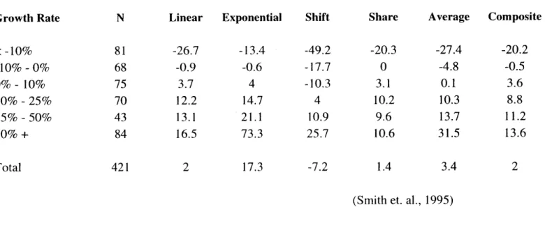
b. Temporal changes in population/employment / Projection. The strengths and
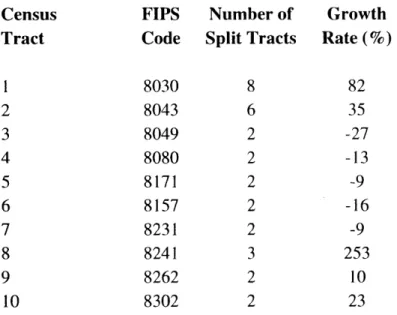
weaknesses of Japanese and U.S. census data formats when applied to temporal analyses, as well as the feasibility of population projections using local census areas for non-census years is discussed in these works. Okudaira (1982) emphasizes that a major advantage of grid squares is the stability of their boundaries over time. Smith and Shahidullah (1995) as well as Tayman (1992) explore various methods of projecting populations for census tracts. Projections become more difficult as census areas become more disaggregated, because small areas are subject to higher enumeration errors. Howenstine (1993) addresses the problems caused by changing physical characteristics of U.S. census tracts over time. Census tracts are supposed to have visible boundaries such as roads and contain between 2,500 and 8,000 people for an average of 4,000. Their boundaries may shift, and tracts may be merged or split in order to account for changes in infrastructure and population. Since split tracts are more frequent than the other two changes, methods
to reconcile the different representations are discussed. It is concluded that leaving the recently split tracts intact and splitting the previously aggregated corresponding area by proportion of populations in the new tracts performs the reconciliation with the smallest deviation from the actual breakdown.
c. Demand forecast along a transit route. Foot (1981) provides a textbook-like
explanation for urban models, including gravity models. In Chapter 6, the gravity model is described in detail, and is adapted for the implementation of census data.
d. Usage of local transit stops. Azar and Ferreira (1995) outline the Period Route
Segment (PRS) model which forecasts transit ridership for each defined traffic analysis zone (TAZ). Here, U.S. census data block groups are implemented to create the TAZs. Chapter 7 discusses the prospects of applying Japanese mesh data to a local transit model such as the PRS.
2.4 Discussion
The examination of the literature enabled an understanding of 1) U.S. and Japanese census data formats' methodology; 2) common issues and problems faced by spatial data users in general; 3) previously tried approaches to the four proposed urban problems, within the U.S. census data context; and 4) tools, such as procedures and techniques, that may facilitate the analyses of the proposed problems. These materials will be restated more thoroughly in later chapters.
This thesis contributes to previous works as a comparative discussion of two census data formats within the context of the proposed urban problems and, more generally, the broader categories of problems. As conclusions regarding the relative suitability of both census formats and the feasibility of tools are drawn for categories of problems, it is
hoped that such conclusions can be helpful in approaching different problems that fall into these categories.
Chapter 3:
The Census Data Formats Examined
This chapter is an overview of the two areal representations, the Japanese and United States census data formats. Historical forces that led to the current formats is described. Then, the definitions of geographic entities which are relevant in this paper, as well as the hierarchies that relate the geographic entities are presented. Finally, a general discussion of data analysis issues that arise from these definitions is presented. These issues will be examined closely within the context of specific urban studies and planning problems later on.
3.1 Japanese Census Data Format
3.1.1 Early Versions of Japanese Census Data
The statement below by social scientist Toshio Sanuki in 1969 is a representative opinion of the times that advocated the creation of what is today called "mesh data" in Japan.
Creative strategic maneuvers are necessary in order to respond to the challenges of the twenty first century and emerge victorious. Formulation of strategy begins with a close look at today's reality. A reorganization of the nation's regional statistics and data, the fundamental material needed to judge this reality, is essential in order to realize the future goals on the Japanese archipelago. Previous regional statistics have been compiled and tallied for a political jurisdiction, primarily for use by that district. It can be said that such data served its purpose of sufficiently fulfilling municipal needs. However, due to rapid changes taking place in our nation, there exists now a need to analyze large regions that transcend municipalities, as well as to examine small parcels within municipalities. Prefectural and municipal data is thus insufficient for projecting future national land use, implementing planning and development strategies. Furthermore, if national land development of the future must incorporate the fourth dimensional element called "time", the data itself must be of a consecutive and consistent nature over a long period of time.' Regional statistics incorporate various information of a particular region and tally the information by tracts, or unit areas. Political jurisdiction were common unit areas in
war Japan. Japan was a nation of many villages, and their boundaries were often clear and unquestioned, often demarcated by nature as well. The numbers of towns and villages decreased with modernization, but the biggest dip occurred in 1953 as a result of the Town-Village Annexation Ordinance being implemented. These events proved very inconvenient for people utilizing regional statistical data, as the statistical unit areas became too large, and time series analyses became impossible.
It had become evident that division of regions according to historical, natural and political perspectives had its limits in terms of consistency and continuity. If such traits are important, regions must be mechanically divided by equidistant horizontal and vertical lines. The congruent squares that result from such a procedure would form the basis for this new grid, or "mesh" system.
It is generally agreed that the Finnish geographer J.G. Gran6 was the first to utilize the mesh system in the scholastic arena. In 1929, he presented a paper on the regional analyses of various natural and anthropological trends using a lkm2 mesh system. Since then, mesh users have gradually increased, and its merits are being recognized.
3.1.2 Creation of "Mesh" Census Data in Japan
In Japan, census data is commonly referred to as "mesh data". Other names include 'grid', 'cell', 'grid square system', 'block grid system', and 'grid coordinate system. One can imagine a grid created by vertical and horizontal lines, all 1 kilometer apart. The lkm2 squares created by this "mesh" system serve as the fundamental regional unit. Thus, any point in the country belong to one of the 386,522 mesh squares.
This is not to say that actual census surveys are conducted with the mesh as a research unit. Each enumerator conducts census research in an area of approximately 50 households and physically resembling a U.S. census block group. The mesh squares are an aggregation of these research units which are "fitted" into the rigorous mesh square. To resolve disputes involving the research units that lie over mesh boundaries, various
techniques have been implemented in different census years, and it is generally conceded that all such techniques are imperfect and that errors will result.
Since the mesh system was introduced for census data in 1970, the census has been conducted every five years (1970, 1975, 1980, 1985, 1990). In previous years, the bureau had conducted census surveys, but the data had been tallied with fundamental regions falling along municipal boundaries and natural barriers. In the 1960's, with the nation experiencing rapid economic growth, demand rose for a new type of data that would allow forecasting and optimizing of infrastructure projects. It quickly became clear that existing forms of census data was not very useful. Among the reasons given were:
(1) since boundaries of municipalities changed with time (including revamping of
municipal hierarchies, mergers, etc..) , a time series analysis of a given region could not be performed,
(2) data in which the fundamental regions are mechanically and equally created are easier to handle, when performing comparisons of regions, as well as when calculating for the cumulative totals of several meshes,
(3) the mesh nature facilitates numerical labeling and orderly mapping of meshes.
Once the creation of the mesh system was justified, the actual procedure for creating the mesh squares was discussed. It was eventually agreed that a grid using lines parallel to longitudinal and latitudinal lines would be the best procedure. It should be noted here, however, that while latitudinal lines are equidistant everywhere, spacing between longitudinal lines becomes smaller as one travels north in the northern hemisphere (thus these lines are actually not parallel). Therefore, mesh areas will not be constant as one travels northward and southward. Comparing the northern and southern extremes, there is a 16% area difference between meshes in the metropolitan Sapporo and metropolitan Kagoshima areas. Between Tokyo and Kita-Kyushu, where the core of Japanese economic activities lies, the error is merely 2.5%. Nevertheless, this longitude-latitude
system was selected over other coordinate systems (UTM, 17-coordinate systems) due to our general familiarity with longitudinal and latitudinal lines.
Mesh hierarchy and mesh labels (called mesh codes) were created as follows. Each 1 km2 mesh has a corresponding 8 digit mesh code. The first 4 digits denote the level I mesh group (each level I mesh is approximately 80 km by 80 km, thus consisting of exactly 64 level II meshes, each approximately 10 km by 10 km), the next 2 digits denote the level II mesh group (1 through 64), and the last 2 digits denote the level III, or fundamental mesh (there are 100 fundamental mesh squares in one level II mesh).
The longitudinal lines are drawn at each degree (123'E through 149'E). In central Japan, these lines are approximately 80 km apart. The latitudinal lines are drawn at 40
minute intervals (36', 36'40', 370201,...), and these lines are approximately 80 km apart.
Thus, a level I mesh group is created by adjacent latitudinal and longitudinal lines. As stated earlier, the first 4 digits correspond to the level I mesh. Of these, the first 2 digits are calculated as follows:
LATITUDE x 1.5
The next 2 digits are derived as follows:
LAST 2 DIGITS OF LONGITUDE
In Figure 3-1, the 4 digit code is given as 5 4 3 8. The lines that intersect at the lower left corner of each level I mesh is used for the calculations.
Next, each level I mesh is subdivided into 64 squares of 10 km by 10 km (level II meshes). Each is labeled, from 00-07, 10-17, 20-27,... to 70-77 as illustrated. The level II mesh in Figure 3-2 would have the code 5 4 3 8 - 2 3. Finally, each level II mesh is subdivided into 100 squares of 1 km2 each (fundamental meshes, or level III meshes). Each is labeled from 00 to 99 as illustrated. The level III mesh in Figure 3-3 would have
Figure 3-1 through 3-3
3.1
The Mesh System
1360
137'0 1380 1390 140'0
38
370 20'360
40'
36*
350 20'Region A is a Level I Mesh Square # 5 4
3 8
5 4 =
36 x 1.5;
3.2
40'
3 8
=
lower two digits of longtitude on the west side
Region B is a Level II Mesh Square # 5 4
3 8 2 3
Each Level II Region corresponds to one 1/25000 scale topographical
map
70
77
60
50
40
30
20
10
00
01 02
03
04
05
06
07
3.3
90
80
70
60
50
|
5
40
30
20
10
00 01 02 03 04 05 06
07 08 09
7' 30"
Region C is a Level III Mesh Square #
5 4
3 8 2 3
5
2
Furthermore, the Bureau of Statistics has compiled a level IV mesh system (500 m by 500m meshes) for selected metropolitan areas, which simply involves a subdivision of the fundamental meshes into 4 squares.
In Japan, the national census data and the national business establishment data are compiled in the mesh system every five years. The national business establishment data lags by one year, so the latest business establishment data set was compiled in 1991. All of the fields that appear in the data sets are summarized here (Table 3-2).
3.1.3 Basic Processing of Mesh Data
The characteristics of mesh data make it suitable for the following procedures, among others, to be performed.
SIMPLE CALCULATIONS. Since the mesh squares are assumed to be congruent, many
types of calculations within a mesh or encompassing multiple meshes are possible. In an example of mesh census data, the population which is not part of the labor force (NLP) is calculated by adding the values of two fields:
NLP = [night population under 15] + [night population over 65]
It is easy to obtain this figure for each mesh. Furthermore, the density of NLP over a particular area can be calculated by adding each NLP and then dividing that figure by the number of cells. Other calculations can be made using the values of other fields, or categories, in the census.
GEOMETRIC QUERY. Occasionally, there arises a need to select a sub-region of a certain shape (square, circle) from some region. For example, a circular region is cut to select the areas which are affected by some poisonous spillage that emits fumes equally in all directions. Although the square shape of each mesh is somewhat limiting, the ideal shape can be closely imitated.
CALCULATING DISTANCE. If two mesh of coordinates (xi , yi ) and (xj , yj ) are given, the distance between them can be calculated as the following:
Table 3.2
Complete List of Tabulations: 1985 Census Data Name of survey
Survey year Mesh code
Mesh level (I thru IV)
1/25000 Map of the Level II mesh corresponding to mesh
Number of cities, wards, towns and villages within mesh Prefectural and city codes for each municipality within mesh
Night population (Total, Male, Female; the same for all fields below) 0-4 years old 5-9 years old 10-14 years old 15-19 years old 20-24 years old 25-29 years old 30-34 years old 35-39 years old 40-44 years old 45-49 years old 50-54 years old 55-59 years old 60-64 years old 65-69 years old 70-74 years old 75-79 years old 80-84 years old 85 years old and over
0-2 years old 0-5 years old 3-5 years old 6-1 years old 12-14 years old 15-17 years old 18 years old 19 years old Labor force Employed workers Totally unemployed Non labor force
Hired personnel (including management) Business owner
Member of family business Type I sector personnel Agricultural personnel Forestry personnel Fishery personnel Type 2 sector personnel Mining personnel
Construction personnel Manufacturing personnel Type 3 sector personnel
Electric/Gas/Heat/Water personnel Transport/Communication personnel Small distributor/Restaurant-Bar personnel Financial/Insurance personnel
Real Estate personnel Service industry personnel Civil Service personnel
Professional/Technical personnel Management personnel
Office Administrative personnel Sales personnel
Agri/Forestry/Fishery worker Construction worker
Transport/Communication worker
Technician/Manufacturing worker/Other worker Security Service worker
Service industry worker (No more tabs by sex)
Commuters 15 years old and over (work, school) Persons working at home
Commute within city, ward, town or village (work, school) Commute within prefecture but different municipality (w, s)
Commute outside prefecture (w, s) Total households
General household Normal household Sub-household
One person household (general, normal) 2,3,4 person household (g, n) 5,6,7+ person household (g, n) Type of household Extended household Nuclear household Other
Household with relative under 6 years of age Household with relative over 65 years of age Condition of household
All commuters, with school commuter under 12 years of age All non-commuters are senior citizens
All non-commuters are either senior citizens or small children
Household supported by Agri/Forestry/Fishery
Household supported by Agri/Forestry/Fishery and other sector Household not supported by Agri/Forestry/Fishery
Type of abode Single home Nagaya (tenement)
Multiple family (1-2 floors, 3-5 floors, 6+ floors) Ownership
Households living in an abode Households living in an owned home Households living in public housing Households living in rented housing Households living in company housing Households renting within a home
Households renting within a home, I person household Male/Female ratio
Average age
Percentage of pre-adolescents
Percentage of persons at a 'productive' age Percentage of senior citizens
Percentage of labor force Percentage of working people Percentage of working females Percentage of hired people
Percentage of people who own businesses Percentage of working people in Type I sector Percentage of working people in agriculture Percentage of working people in Type 2 sector Percentage of working people in construction Percentage of working people in manufacturing Percentage of working people in Type 3 sector
Percentage of working people in small distributor/small store/restaurant/bar Percentage of working people in service industry
Percentage of working people in professional /technical /managerical /administrative position Percentage of workers as technicians, manufacturing and other labor positions
Percentage of workers in sales and service Percentage of commuters
Percentage of commuters to other municipalities Percentage of nuclear households
Percentage of households with children under 6 years of age Percentage of households with people 65 years of age and over Percentage of single homes
Percentage of nagaya
Percentage of purchased homes Percentage of public housing Percentage of rented home Number of rooms per household Number of tatami mats per household Average member per household Number of rooms per person Number of tatami mats per person
Complete List of Tabulations: 1981 Business Establishment Data Name of survey
Survey year Mesh code
Mesh level (I thru IV)
1/25000 Map of the Level II mesh corresponding to mesh
Number of cities, wards, towns and villages within mesh Prefectural and city codes for each municipality within mesh
(All categories have two fields: Number of facilities, Number of employees, unless otherwise noted)
All industries
Type 2 sector industries Mining Construction Manufacturing Light industry-materials Light industry-processing Heavy industry-materials Heavy industry-processing Chemical industry Other industry
Type 3 sector industries Small distributor-retail Small distributor Small retail Textile/Clothing distributor Restaurant-Bar distributor Restaurant-Bar Financial/Insurance Real Estate Transport/Communication Electricity/Gas/Water/Heat Service Laundry/Cosmetic Medical Education Social insurance/welfare Life services
Medical/Sanitary/Welfare related services Entertainment related service
Administrative related service Civil Service Manufacturing 1-9 employees Manufacturing 10-29 employees Manufacturing 30-99 employees Manufacturing 100-299 employees Manufacturing 300-499 employees Manufacturing 500-999 employees Manufacturing 1000+ employees Distributors/Retail 1-9 employees Distributors/Retail 10-29 employees Distributors/Retail 30-49 employees Distributors/Retail 50-99 employees Distributors/Retail 100-299 employees Distributors/Retail 300+ employees
Service 1-9 employees Service 10-29 employees Service 30-49 employees Service 50-99 employees Service 100-299 employees Service 300+ employees All industries 1-4 employees 5-19 employees 20-29 employees 30-49 employees 50-99 employees 100-299 employees 300+ employees Management practice Self Corporate Public Business Format Store/Restaurant-Bar Office Factory/Plant/Works Time of Founding Before 1944 1945 -1954 1955 -1964 1965- 1972 1973- 1978 1979 and thereafter
Average number of employees
All industry Manufacturing Supplier/Retail Service Proportion by industry Manufacturing Distributor/Retail Service
Proportion by time of founding before 1954
1955- 1972 1973 and thereafter
dij = { (x i -xj )n + (y .. yj )n}1l/n
n=2 when direct travel is possible, and n=1 when only horizontal and vertical movements are possible.
3.2
U.S. Census Data Format
A long tradition of census taking exists in the United States, beginning from its
colonial period. One-time enumeration in the colonies of Virginia (1624), New York
(1712), Connecticut (1756), Massachusetts (1764) and Rhode Island (1774) were
conducted at the request of the British for administrative purposes. However, guidelines that defined the purpose of the modern U.S. census was outlined in the U.S. Constitution, adopted in 1787. The cost of fighting the Revolutionary War had been high, and each State was to contribute to the common defense of the new nation on the basis of their populations. The new constitution also defined an electoral system where States would be represented in Congress on the basis of their populations. The Constitution required the President of the Union to conduct a popular census every ten years.
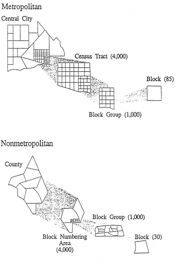
The U.S. census is still conducted once every ten years, and has a stated mission of acting as a tool to redefine electoral districts. The data structure hierarchy is illustrated in Figure 3-4. It is evident that the hierarchy contains numerous geographic entities, for
various purposes. In later chapters, the census tracts, block groups and blocks will be the entities that will receive much discussion. The Japanese Level III mesh squares have an average population of 749 throughout Japan (1985) although the range is very wide. This geographic entity is the least aggregated level where data for the entire country is available. Since U.S. block groups average 1,000 people, this entity arguably is a sound choice for comparative purposes. Census tracts are important, as they are the entities of choice for many spatial analyses, because of MAUP, and for relative simplicity. These entities are briefly described here (U.S. Bureau of the Census, 1990). Their spatial relationships are illustrated in Figure 3-5.
Figure 3-4 Hierarchy of U.S. Census Geographic Entities
(Number inside parentheses denote mean population)Metropolitan
Central City .
Census Tract (4,000)
Block
(85)
Block Group (1,000)
Nonmetropolitan
County
Block Numbering
Area
(4,000)
Block Group (1,000)
Block (30)
23
Census Tracts - Census tracts are small areas with generally stable boundaries, defined within counties and statistically equivalent entities, usually in metropolitan areas and other highly populated counties. They are designed by local committees of data users to be relatively homogeneous with respect to population characteristics, economic status, and living conditions at the time they are established. Census tracts average 4,000 persons, but the number of inhabitants generally ranges from 2,500 to 8,000 persons.
Block Groups (BG's) -BG's are combinations of census blocks within census tracts and Block Numbering Areas (BNA's are the non-metropolitan equivalent of census tracts).
All the blocks in a BG have the same first digit in their identifying numbers; e.g., BG 4
contains all blocks numbered from 401 to 499 in a census tract or BNA. The entire nation and its territories are subdivided into blocks for the first time in the 1990 census.
Blocks -These are the smallest geographic units for which the Census Bureau tabulates data. For the 1990 census, the Census Bureau numbered blocks throughout the nation and its territories for the first time. Many 1980 census blocks were revised and renumbered to meet the requirement that their boundaries follow visible features such as streets, streams, and railroad tracks, as well as to reflect new and corrected street patterns. Unlike the 1980 census, blocks are not split between geographic entities; rather, a unique three-digit block number, sometimes with an alphabetic suffix, applies to each entity. For example, the 1980 census reported data for the place and nonplace portions of block 101; in the 1990 census, there are data for two specific block numbers: lOA inside the place and 1OB outside. For the 1990 census, the entire United States and its territories were divided into more than 7 million blocks. For the 1980 census, data were tabulated for only 2.5 million blocks; in nonblock-numbered areas, the ED, usually covering a much larger area than a block, was the smallest area for which the Census Bureau tabulated data.
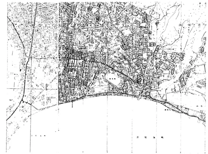
Census Tracts are Defined Using Physical Boundaries
An important feature of the U.S. census to be pointed out at this stage is that an effort is made to keep the average populations at census tract and block group levels more or less constant. This means that boundaries at those aggregation levels can and will change. This is one feature which differentiates the U.S. data set considerably from that of Japan.
3.3 Comparing Inherent Characteristics of the Two Representations
It can be argued that many of the differences between the census processes in the two countries stem from the different motives and conditions for taking the census. As stated earlier in this paper, the mesh format of the census data in Japan was introduced as an analysis tool to estimate and optimize social and economic growth. In comparison, the
U.S. census tracts and block groups are created with a degree of population homogeneity
and enumeration ranges as goals, so their areas may change over a period of time.
The mechanical nature of the mesh system does not take into account the various "exceptions" that occur in any landscape, which can prevent one mesh square from reflecting the characteristics of the greater area of its vicinity. An example of such a situation is the park situated amidst a downtown business district. If a mesh happened to be situated directly over that park (assuming that the park is approximately 1km2), that mesh would not possess many of the characteristics of the surrounding cells. While this aberration would be treated at face value for certain analyses, the characteristic of the larger surrounding city blocks may be desired for other analyses. Further, an artificial smoothing of the aberrational and surrounding mesh squares to dampen the contrast may or may not be feasible, depending on the nature of the problem.
Another issue particular to the Japanese mesh system is the formula for assigning each census research unit of approximately 50 households to each mesh square. Over the years, various formulas have been implemented to assign those research units that were split by mesh boundaries. With the majority of these formulas, it can't be helped that the
resulting mesh squares really aren't true squares; the rigorous nature of the square will always be compromised by the shape of the smaller research units themselves. Nevertheless, the mesh are assumed to be perfect squares, resulting in a difference between the TRUE nature of the area within the perfect square, and the REPRESENTATION of that same area using mesh. This represents a problem when a high degree of accuracy in individual mesh representation is of the researcher's highest priority.
Chapter 4:
Counting of Populations Using Census Data
This chapter discusses the procedures and the issues that arise when Japanese and U.S. census data are applied to perform population counts of a specified area such as municipalities, neighborhoods, or electoral districts. Chapter 3 described the concept of dividing the U.S. and Japan into geographic entities that spatially represent all areas, but the process of assigning attribute data, such as population, to these geographic entities is not a trivial task. This assignment process, as well as the nature of the geographic entities themselves, significantly affect the enumeration process for both census formats.
4.1 Methods for Counting People
An array of methods that exist throughout the world for a population count can be generalized into three types. In places where no on-ground tabulations are available or collected, the areal extent of an urbanized area gained from satellite images is used to estimate population. This is often used in cities of the developing world, and is associated with some obvious problems. The expected level of error becomes quite significant at local levels and it is virtually useless for counts of sparsely populated areas. Information regarding socio-economic and demographic breakdowns, as well as temporal changes cannot be obtained. However, this may be the only available method for estimating population in countries where neither a census is held nor a population register is maintained.
Residents of most western European countries and Japan, among others, submit information to local population registers. Such registers, normally administered by municipalities, hold information regarding individuals' postal address as well as typical identifiers such as name, birth date, sex, marital status and unique identification numbers. Therefore, a municipality always will refer to their own population registry for questions
regarding its population. Such registers can maintain high accuracy only if residents dutifully report changes, typically changes of address, marriage, births and deaths. Many countries use the tactic of forced encouragement in order to update registry information. For example, some countries use the registry to identify and send out social security payment information, and others may use the registry to identify women of certain ages who need to be informed of cancer screening procedures. The extreme case of absolute reliance on registry data for population statistics is Denmark, where traditional census activities have been abandoned in favor of 37 registries that hold statistics for the national population. The high accuracy level of their registries is reflected by the generally satisfactory level of public service delivery. Accuracy of these registers differ among countries, however. The Swedish register and census data from 1980 revealed that only
0.3 percent of people recorded in the registers were recorded incorrectly. On the other
hand, Italians and Spanish have been known to be slow to notify changes. In Japan, where registry statistics are known to be highly accurate (updating is considered very important, as this information is necessary for school/job application, social services, marriage, and other various activities), address-linked population counts can theoretically be performed using these figures, although the data is completely closed from public access.
The third method of discussion is that of counting using census data. In the case of Japan, it has already been established that its registry is highly accurate, and queries such as population figures for incorporated municipalities can be satisfied with very high accuracy; the limitations of the rigorously defined census mesh squares to handle natural and political boundaries has been discussed. However, when performing population counts of municipal sub-areas or areas that are specified by other boundaries, the use of the registry becomes quite a complex task. First, the registry data must be related spatially in order to query only the records within the specified boundary. This may be manageable for small areas at a time, but considering that each Japanese resident is