A new numerical method for axial dispersion characterization in microreactors

HAL Id: hal-01767280

https://hal.archives-ouvertes.fr/hal-01767280

Submitted on 16 Apr 2018

HAL is a multi-disciplinary open access

archive for the deposit and dissemination of

sci-entific research documents, whether they are

pub-lished or not. The documents may come from

teaching and research institutions in France or

abroad, or from public or private research centers.

L’archive ouverte pluridisciplinaire HAL, est

destinée au dépôt et à la diffusion de documents

scientifiques de niveau recherche, publiés ou non,

émanant des établissements d’enseignement et de

recherche français ou étrangers, des laboratoires

publics ou privés.

A new numerical method for axial dispersion

characterization in microreactors

Maxime Moreau, Nathalie Di Miceli Raimondi, Nathalie Le Sauze, Christophe

Gourdon, Michel Cabassud

To cite this version:

Maxime Moreau, Nathalie Di Miceli Raimondi, Nathalie Le Sauze, Christophe Gourdon, Michel

Cabas-sud. A new numerical method for axial dispersion characterization in microreactors. Chemical

Engi-neering Science, Elsevier, 2017, 168, pp.178-188. �10.1016/j.ces.2017.04.040�. �hal-01767280�

To cite this version : Moreau, Maxime and Di Miceli Raimondi, Nathalie and

Le Sauze, Nathalie and Gourdon, Christophe and Cabassud, Michel A new

numerical method for axial dispersion characterization in microreactors.

(2017) Chemical Engineering Science, vol. 168. pp. 178-188. ISSN 0009-2509

O

pen

A

rchive

T

OULOUSE

A

rchive

O

uverte (

OATAO

)

OATAO is an open access repository that collects the work of Toulouse researchers and

makes it freely available over the web where possible.

This is an author-deposited version published in :

http://oatao.univ-toulouse.fr/

Eprints ID : 19834

To link to this article :

DOI : 10.1016/j.ces.2017.04.040

URL :

http://dx.doi.org/10.1016/j.ces.2017.04.040

Any correspondence concerning this service should be sent to the repository

administrator:

staff-oatao@listes-diff.inp-toulouse.fr

A new numerical method for axial dispersion characterization in

microreactors

Maxime Moreau, Nathalie Di Miceli Raimondi

⇑

_{, Nathalie Le Sauze, Christophe Gourdon, Michel Cabassud}

Laboratoire de Génie Chimique, Université de Toulouse, CNRS, INPT, UPS, 4 Allée Emile Monso, F-31432 Toulouse, France

h i g h l i g h t s

!An innovative numerical method for axial dispersion characterization is proposed.

!The method is validated thanks to a RTD experiment in a microchannel.

!The method is applied to rectangular millimetric wavy channels.

!The impact of the channel geometry on the axial dispersion coefficient is studied.

Keywords: Axial dispersion Numerical method CFD simulations Microreactor Wavy channel

a s t r a c t

Axial dispersion is a key phenomenon in reactor engineering that can affect yield and selectivity when reactions are carried out. Therefore its characterization is necessary for an adequate modelling of the reactor. The development of compact reactors to fit with process intensification expectations requires the use of characterization methods adapted to small-scale devices. An original method not-frequently used up to now for the estimation of axial dispersion coefficients is presented and applied to millimetric wavy channels. It is based on CFD simulations to calculate velocity and concentration fields from which axial dispersion coefficient can be estimated. This method is used to predict the impact of the wavy chan-nel geometry and of the fluid velocity on axial dispersion in laminar flow regime. The investigated geo-metrical parameters are the hydraulic diameter (2–4 mm), the cross-sectional aspect ratio defined as the ratio between the channel width and its depth (0.25–1) and the internal curvature radius of the bends (2– 3.4 mm). The range of Reynolds number considered is Re = 70–1 600. Axial dispersion coefficient increases with velocity, values range from 2.8 " 10#4_{to 3.2 " 10}#3_m2_"s#1_{. It appears that axial dispersion}

varies slightly in function of the channel hydraulic diameter. Square wavy channels generate less axial dispersion than rectangular wavy ones. Finally, axial dispersion coefficient increases with the internal curvature radius which shows the positive impact of sharp bends to reduce axial dispersion effect.

1. Introduction

At the core of chemical engineering, reactor design is funda-mental to reach a goal of productivity. A rigorous management of the operating conditions (flow rate, temperature, pressure, etc.) is notably necessary to limit the production of by-products and to carry out the reaction safely (Nikacˇevic´ et al., 2012). It requires the control of the different transfer mechanisms related to mixing, heat transfer and mass transfer in homogeneous or heterogeneous media. For that purpose, fine chemistry and pharmaceutical indus-tries usually slow down the intrinsic kinetics (dilution, low tem-perature, fed-batch operation, etc.) so that the process is not

limited by the kinetics of transport phenomena. In a concern of a greener chemistry, process intensification advocates since a few years the development of technologies which adapt themselves to the implemented chemistry and not the opposite (Van Gerven and Stankiewicz, 2009). The objective is to work under adequate operating conditions that ensure a safe process, limit the use of sol-vents and optimize energy consumption (notably by means of the reduction of operations that follow reaction such as separations and waste treatments). The intensification of the chemical reactors is often envisaged for the implementation of exothermic reactions, since a bad control of the temperature may degrade the production and even worse, cause serious damages due to thermal runaways. Today, numerous technologies of intensified reactors are available among which microreactors (Anxionnaz et al., 2008; Lutze et al., 2010). They offer an important exchange area compared to the vol-⇑Corresponding author.

ume of the reactor for an enhancement of heat transfer. The reac-tive fluid circulates generally at moderate velocity to provide enough residence time for the reaction. So, due to the low size of the intensified devices and the low velocity of the fluids, flow regimes are often laminar in microreactors. Therefore, to ensure a fast contact between reactants, these technologies are commonly designed according to complex geometries in order to intensify mixing despite laminar flow. It results in particular hydrodynamic behaviours (Amador et al., 2008; Boskovic and Loebbecke, 2008; Moreau et al., 2015) that need to be characterized in order to detect possible flow defaults. Global hydrodynamic characteriza-tion of reactors also gives informacharacteriza-tion about the global hydrody-namic behaviour of a device (from the plug flow to the perfectly stirred tank character) for an adequate modelling of the reactor (Levenspiel, 1999). The objective is then to obtain a reliable esti-mate of conversion rate and selectivity. Tubular reactors are gener-ally modelled as plug flow reactors with axial dispersion. In a perfect plug flow, all the fluid elements have the same residence time. Axial dispersion reflects the heterogeneity of the residence times due to molecular diffusion, velocity profile, turbulence, dead zones and other flow defaults.

The dispersion model consists in a one-dimension equation resulting from the projection along the main direction of the flow of the general transport equation of a chemical species in an incompressible fluid (convection-diffusion equation). In steady state, for a reactant A, this model can be written as follows:

huzi

dhCAi

dz # Dax d2hCAi

dz2 # rA¼ 0 ð1Þ

where huzi and hCAi are respectively the velocity and the concentra-tion of A averaged over the reactor cross-secconcentra-tion, Daxis the axial dis-persion coefficient, rA is the rate of reaction of A and z is the coordinate along the main direction of the flow.

The present article describes and discusses classical methods to estimate axial dispersion coefficients in a device and focuses on an original method based on simulations. The method is then applied to characterize microreactors that consist of millimetric wavy

channels of different cross-section shapes and dimensions. The objective is to evaluate the impact of the channel geometry on axial dispersion with an objective of process scale-up.

2. Methods for axial dispersion characterization 2.1. Models for axial dispersion coefficient estimation

Models exist to estimate axial dispersion coefficient in tubular reactor, according to the device geometry and the flow regime related to Reynolds number (Eq.(2)):

Re ¼

q

huzidH

l

ð2Þ

For laminar flow in tubular pipes (Re < 2100),Taylor (1953)and Aris (1956) established a relation between the axial dispersion coefficient, the molecular diffusion coefficient, the hydraulic diam-eter and the average velocity (Eq.(3)).Squires and Quake (2005) and Ajdari et al. (2006) proposed similar correlations for non-circular pipes.

Dax¼ Dmþhu zi2d2H

192Dm ð3Þ

However, this model is only applicable when the characteristic time of axial convection is very high compared to the characteristic time of tangential diffusion (i.e. a molecule entering the center of the pipe must have enough time to migrate to the wall by diffusion before leaving the pipe). This condition can be written in terms of Eq.(4)(Nagy et al., 2012).

L huzi > 0:04d 2 H Dm ð4Þ

Mathematical models can also be used in laminar flow using pure convective Residence Time Distribution theory (Wörner, 2010). These models are applicable for fully developed flows in Nomenclature

C concentration (mol"m#3₎

hCi averaged concentration over the cross-section (mol"m#3₎

~

C spatial fluctuation of the concentration (mol"m#3₎ Dax axial dispersion coefficient (m2"s#1)

De Dean number

dH hydraulic diameter (m)

dl element of length (m) ds element of surface (m2₎

Dm molecular diffusion coefficient (m2"s#1)

Ds spatial dispersion coefficient (m2"s#1)

E distribution function (s#1₎ F ! external forces (N"m#3₎ I identity tensor J !

diffusive flux (mol"s#1_"m#2₎ l channel depth (m) L reactor length (m)

Ls straight length between two bends (m)

n

!

unit normal vector P pressure (Pa) Q flow rate (m3

"s#1) r rate of reaction (mol"m#3

"s#1) Rc curvature radius (m) Re Reynolds number S cross-section (m2₎ Sc Schmidt number t time (s) u ! velocity vector (m"s#1₎

huzi averaged velocity over the cross-section (m"s#1)

~

uz spatial fluctuation of the axial velocity (m"s#1)

w channel width (m)

z coordinate according to the main direction of the flow (m)

Greek letters

q

density (kg"m#3₎

l

dynamic viscosity (Pa"s)

dS boundary (perimeter) of the section S (m) dtetraheral size of the tetrahedral mesh grid (m)

dcubic size of the cubic mesh grid (m)

a

cross-sectional aspect ratio of the channel

s

viscous stress tensor (Pa)

Subscripts

exp experimental result mod calculated with a model simu simulation result

circular or rectangular channels with fluids characterized by very high Schmidt number (Sc ¼

l

=ð

q

DmÞ) so that dispersion by molec-ular diffusion can be neglected.

In turbulent regime (Re > 3000) and for straight circular pipes the relationship between the axial dispersion coefficient and Rey-nolds number is written as follows (Trambouze and Euzen, 2004):

Dax huzidH¼ 3 " 107 Re2:1 þ 1:35 Re0:125 ð5Þ

These models are applicable to simple geometries with limited velocity ranges or very long lengths (see Eq.(4)) while microreac-tors consist generally in short complex channel patterns to enhance mixing and transfer performances despite laminar flow condition. Therefore, experiments or simulations are generally required to characterize axial dispersion in a particular reactor.

2.2. Experimental methods

Axial dispersion coefficient is mainly estimated from Residence Time Distribution (RTD) experiments. The protocol consists in the injection of a tracer into the main fluid. The injection may not dis-turb the flow nor modify the physicochemical properties of the main fluid. It is detected at the reactor input and output. The obtained inlet and outlet signals are then analyzed in order to cal-culate the mean residence time inside the reactor and the axial dis-persion coefficient (Levenspiel, 1999). The choice of the tracer depends on the analysis method. The main methods for liquid phase tracing are given below:

- Radioactivity (Kolar et al., 1987; Blet et al., 2000; Lelinski et al., 2002; Borroto et al., 2003): the main advantage of radioactivity measurements are the good accuracy (high detection sensitiv-ity) and the fast response time of the sensors. However, this method is not-frequently used in liquid phase tracing due to the price of radioactive tracers and the risk of contamination and irradiation. It is more common for gas phase RTD where other types of tracer are not soluble.

- Thermal tracing: despite the simplicity of this method and its low cost, it is rarely used because it is intrusive (temperature sensors in the flow). The response time is high (thermal inertia) and the signals are highly disturbed notably by thermal losses and conduction in materials.

- Conductivity detection (Sancho and Rao, 1992; Gutierrez et al., 2010; Mohammadi and Boodhoo, 2012): this method is widely used because it is easy to implement at moderate cost. How-ever, limitations exist for application in micro-devices diagno-sis: the intrusive character of the method, the size of the probes and their response time (generally a few seconds). How-ever new devices are proposed in response to these limitations such as wire-mesh sensors (Elias and Rudolf von Rohr, 2016; Häfeli et al., 2013).

- Optical detection: although the material is expensive and frag-ile, optical detection (e.g. UV–vis spectrophotometry (Boskovic and Loebbecke, 2008; Adeosun and Lawal, 2009; Günther et al., 2004; Kurt et al., 2015), fluorescence techniques (Lohse et al., 2008)) is very often used in microreactors because the response time of the sensors is of some hundred milliseconds. Moreover, these methods can be non-intrusive as far as the detection zone is transparent.

Even though they are very commonly used, experimental RTD presents significant drawbacks notably for the characterization of microreactors, i.e. devices of small volumes:

- RTD can be sensitive to the injection method since it can locally disturb the flow rate and the pressure. To avoid this effect, for a Dirac-like injection, an injection loop prefilled with tracer should be preferred to a syringe injection. A step-like injection can also be carried out switching from the main fluid to the solution of tracer at the entrance of the reactor. However, both methods require to manipulate valves which can bring air bub-bles in the fluid, leading to a disturbance of the signals. - Processing of the signals is required to take into account the

non-ideality of the entrance signal such as convolution-deconvolution technique (Adeosun and Lawal, 2009; Gutierrez et al., 2010) and the noise related to the analysis method. This processing often generates a loss of information, notably related to the signal trail. This leads to a global underestimation of the axial dispersion.

- The analyzed zone must be representative of the reactor cross-section. This can be problematic if the channel size is larger than the sensor diameter. The use of cross-shape measuring cells can also be considered. In such a cell the fluid flows in a channel with the exact dimension of the probes. However, it leads to supple-mentary volumes (cells and connectors) at the reactor inlet and outlet characterized by their own residence time and axial dis-persion. These secondary volumes can be significant compared to the usual volume of a microreactor, leading to an unreliable estimation of the axial dispersion generated only by the reactor. 2.3. Numerical methods

Thanks to the recent advances in computational capabilities and in CFD softwares (solving algorithms, design and meshing of com-plex geometries), many studies deal with numerical RTD. Two main methods are used:

- Particle tracking (Castelain et al., 2000; Sahle-Demessie et al., 2003; Le Moullec et al., 2008; Bai et al., 2008; Aubin et al., 2009; Habchi et al., 2010): this method is based on the simulation of the transport of Lagrangian particles injected at the reactor inlet at a given time (pulse injection). The trajectory of the parti-cles obeys the force balance. Their characteristics are chosen so that they perfectly follow the elements of fluids (very small diameter and same density as the main fluid). The disadvantage of this method is that the tracer is not submitted to molecular dif-fusion. With a no-slip boundary condition at the reactor walls, particles injected near the walls may leave the reactor after a very long time, notably in laminar flow (Castelain et al., 2000; Bai et al., 2008; Aubin et al., 2009). In real flow conditions, the tracer at the wall would have been tangentially transported towards the reactor core by molecular diffusion. The trapped particles tend to emphasize the trail in RTD curve, leading to an overesti-mation of axial dispersion coefficient. Therefore, the RTD curve is generally truncated (some particles are neglected): the value of the resulting axial dispersion coefficient depends on the per-centage of particles neglected. This method is so consistent when molecular diffusion is negligible compared to the other sources of transport. It may not be the case in confined devices with small characteristic dimensions such as microreactors.

- Tracer transport (Le Moullec et al., 2008): the concentration field of a passive scalar (tracer concentration) is computed by solving the general transport equation. This method is less used than particle tracking since concentration transport introduces numerical diffusion. This artificial diffusion contributes to axial dispersion in simulated RTD, leading to an overestimation of axial dispersion coefficient. Numerical diffusion can be negligi-ble compared to the other sources of dispersion but it generally requires very refined meshes and so highly time-consuming simulations.

As for experimental characterizations, numerical RTD require mathematical processing to identify the axial dispersion coefficient from the outlet signal. This post-processing can lead to significant loss of information. Talvy et al. (2007) proposed an alternative method based on the expression of the different contributions to axial dispersion as function of the velocity and the concentration fields (i.e. molecular diffusion, temporal dispersion and spatial dis-persion) (Talvy et al., 2007; Le Moullec et al., 2008). Therefore, axial dispersion coefficient can be estimated from simulations solving the continuity equation, Navier-Stokes equations and the transport equation of a tracer. This method is described in details in the next section. Its main advantage is that it is not based on RTD and so does not require post-processing techniques (convolution-deconvolution techniques, particles counting, model fitting). How-ever, like any numerical method, an adequate mesh should be used to obtain reliable simulations with negligible numerical diffusion. 3. Description of the numerical method

3.1. Mathematical formulation of the axial dispersion coefficient The method proposed byTalvy et al. (2007)is based on the pro-jection of the transport equation along the main direction of the flow (Talvy et al., 2007). The general transport equation without a source term (i.e. transport of an inert tracer) is expressed as:

@C @tþ

r

" ðu

!

CÞ þ

r

" ð J!Þ ¼ 0 ð6Þ

As illustrated inFig. 1, the main direction of the flow is given by the z-direction. The integral over the section normal to the flow (i.e. channel cross-section) is applied to Eq.(6):

1 S ZZ S @C @tds þ 1 S ZZ S

r

" ðu!CÞds þ1 S ZZ S

r

" ð J!Þds ¼ 0 ð7Þ

The divergence operators can be divided into two contributions: the divergence in the plane normal to the flow (rS") and the derivative in the main flow direction (rz" ðu

! Þ ¼ @uz=@z considering a straight flow): 1 S ZZ S @C @tds þ 1 S ZZ S

r

S" ðu ! C þ J!Þds þ1 S ZZ S @ @zðuzC þ JzÞds ¼ 0 ð8Þ

Then, the divergence theorem is applied. It postulates that the surface integral of the divergence of a vector is equal to the surface boundary integral of the vector flux (dS is the boundary of the cross-section S and n!the normal vector to the boundary in the plan S): 1 S ZZ S @C @tds þ 1 S Z dS ðC u!" n!þ J!" n!Þdl þ1 S ZZ S @ @zðuzC þ JzÞds ¼ 0 ð9Þ

The fluxes through the cross-section boundary, i.e. through the reactor walls, are null. Therefore the second term is null and Eq.(9) can be simplified: 1 S ZZ S @C @tds þ 1 S ZZ S @ @zðuzC þ JzÞds ¼ 0 ð10Þ

Considering a reactor with a constant cross-section, the surface integral and the derivate can be permuted:

@ @t 1 S ZZ S C ds " # þ@ @z 1 S ZZ S ðuzC þ JzÞds " # ¼ 0 ð11Þ

Eq.(12) is then obtained by assuming that the diffusive flux obeys Fick’s law:

@ @t 1 S ZZ S C ds " # þ@ @z 1 S ZZ S uzC # Dm@C @z " # ds " # ¼ 0 ð12Þ

The surface integral is represented by a surface average opera-tor (Eq.(13)). h i ¼1 S ZZ S ds ð13Þ

Therefore Eq.(12)can be written in terms of Eq.(14).

@hCi @t þ @huzCi @z # @ @z Dm @C @z $ % ¼ 0 ð14Þ

Finally, the velocity and the concentration are expressed as the sum of an average value over the cross-section and a spatial fluctu-ation that represents the non-uniformity of velocity and concen-tration across the section:

uz¼ huzi þ ~uz ð15Þ

C ¼ hCi þ ~C ð16Þ

Therefore the term huzCi in Eq.(14)can be expressed as follows:

huzCi ¼ hhuzihCii þ hhuzi~Ci þ h~uzhCii þ h~uzCi~

¼ huzihCi þ huzih~Ci þ h~uzihCi þ h~uzCi~ ð17Þ

The application of the average operator to Eqs.(15) and (16) gives h~uzi ¼ 0 and h~Ci ¼ 0. Therefore, Eq.(17)can be simplified:

huzCi ¼ huzihCi þ h~uz~Ci ð18Þ

The last term of Eq.(18)represents a convective flux per unit area. It is classically modelled as the product between a diffusivity and a concentration gradient (Eq.(19)). In the present case, the term h~uzCi translates the tracer spreading due to the non-~ uniformity of the velocity across the reactor cross-section. There-fore the term of diffusivity Ds is called the spatial dispersion coefficient.

h~uzCi ¼ #D~ s@hCi

@z ð19Þ

It leads to the following expression of Eq.(14):

@hCi @t þ @huzihCi @z þ @ @z #Ds @hCi @z " # #@ @z Dm @hCi @z " # ¼ 0 ð20Þ z y x

δ

S S n _Flow direc+on

Considering a constant cross-section and an incompressible fluid, the average velocity huzi is independent of the coordinate z. Therefore Eq.(20)can be written in terms of Eq.(21)(related to the unsteady general convection-dispersion equation without reaction): @hCi @t þ huzi @hCi @z # @ @z Dax @hCi @z " # ¼ 0 ð21Þ

where Daxis the axial dispersion coefficient given by:

Dax¼ Dmþ Ds ð22Þ

It has to be noticed that stationary laminar flow is considered in this study. With unstationary flow (for instance in turbulent flow), a temporal dispersion coefficient also contributes to axial disper-sion coefficient. It is obtained with an analogous mathematical process than the one described from Eqs. (7) to (22)applying a time average operator at Eq.(6), and by introducing temporal fluc-tuations in Eqs.(15) and (16)(Talvy et al., 2007; Le Moullec et al., 2008).

Eqs.(19) and (22)show that the axial dispersion coefficient can be predicted from the molecular diffusion coefficient and velocity and concentration fields obtained by CFD simulations:

Dax¼ Dmþ Ds¼ Dm#

h~uzCi~ @hCi

@z

¼ Dm#

hðuz# huziÞ " ðC # hCiÞi @hCi

@z

ð23Þ

3.2. Computation method

The simulations were carried out according to two steps using the CFD software Comsol Multiphysics 4.3b: at first, the hydrody-namic behaviour of the system is computed in steady state. In a second step, the concentration field of a solute injected at the channel inlet is determined (transient simulation mode). The method assumes that (1) the main fluid and the tracer are perfectly miscible, (2) they are Newtonian and incompressible, (3) the phys-ical properties of the main fluid are constant and not influenced by the presence of the tracer, (4) the solute concentration does not affect the flow structure.

The main fluid is water (

q

= 1000 kg"m#3_,

_l

_{= 10}#3_Pa"s). Methy-lene blue is often used as a tracer in water using spectrophotome-try technique for its detection. The value of its molecular diffusion coefficient in water is considered in the simulations as being Dm= 6 " 10#10m2"s#1.

3.2.1. Hydrodynamics computation

The velocity field is governed by Navier-Stokes and continuity equations. Their expressions for an incompressible fluid flow in steady state are as follows:

q

ðu!"

r

Þ u!¼

r

" ð#PI þ

s

Þ þ F

!

ð24Þ

q

r

!u¼ 0 ð25Þ

where P is the pressure, I is the identity tensor,

s

is the viscous

stress tensor and F!represents the external forces (corresponding to the force of gravity in this work).

The boundary conditions are as follows: - laminar velocity profile at the channel inlet;

- atmospheric pressure at the channel outlet and normal compo-nent of the stress null (

s

" n!¼ 0);

- no-slip velocity at the walls (u!¼ 0).

3.2.2. Tracer transport computation

The concentration field is obtained by solving the general mass transport equation for an incompressible fluid where the diffusive flux is given by Fick’s law:

@C

@tþ

r

" ð#Dm

r

CÞ þ u

!

"

r

C ¼ 0 ð26Þ

At initial time (t ¼ 0), there is no tracer in the channel:C ¼ 0. The boundary conditions are as follows:

- an injection function CiðtÞ is set at the channel inlet. Its expres-sion is discussed in the next section;

- the conservation of the normal component of the flux at the channel outlet is assumed. In other terms the concentration gradient over the main direction of the flow is zero at the outlet. Regarding Eq.(23), this condition requires that the axial disper-sion coefficient is calculated few cells before the outlet section; - there is no flux through the walls. In other terms the concentra-tion gradient over the direcconcentra-tion normal to a wall is zero at this wall.

3.2.3. Tracer injection function

Unlike RTD experiments, the injection function of the tracer should not be a Dirac or a step. Indeed, regarding the expression of the axial dispersion coefficient (Eq.(23)), it is necessary to avoid the average concentration gradient to be zero at the section where Daxis calculated. Consequently, a linear function of time is used:

CiðtÞ ¼ 0 " 1t ð27Þ

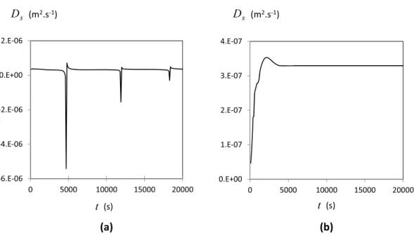
Fig. 2illustrates the impact of the injection function on the cal-culated axial dispersion coefficient. With a Dirac injection (Fig. 2 (a)), the value of Dsis unstable with time while it reaches a plateau when Eq.(27)is applied (Fig. 2(b)). The time to reach the plateau is related to the time required for the tracer to be present in each of the nodes of the section where Daxis calculated. The value of the plateau is the one of interest since the continuous reactors are operated in steady-state.

3.3. Validation of the method in a circular straight capillary 3.3.1. Comparison with Taylor and Aris model

The curves presented inFig. 2are obtained in a straight circular capillary of 2 mm inner diameter and 0.27 m length. The average velocity is 10#4_m"s#1_{. This simple geometry is used in a} prelimi-nary study to set-up and to validate the methodology. Indeed, such a geometry and operating conditions allows to satisfy Taylor and Aris condition given by Eq.(4):

L huzi ¼ 2700 & ' > 0:04d 2 H Dm ¼ 267 " # ð28Þ

The geometry for the simulation consists in a 2D-axisymetric domain. The mesh is composed of uniform quadrilaterals with a size of 50 mm. Such a mesh allows to obtain a grid-independent solution. The axial dispersion coefficient predicted by the simula-tion is Dax;simu= 3.30 " 10#7m2"s#1. Taylor and Aris model expressed in terms of Eq.(3)gives Dax;mod= 3.48 " 10#7m2"s#1. It appears that both values are in a fairly good agreement, with a relative differ-ence of 5.1%.

3.3.2. Comparison with a RTD experiment

A RTD experiment is carried out in a PTFE tube of 2 mm inner diameter. A flow rate of 1.2 mL"h#1_{of water is delivered thanks} to a neMESYS syringe pump. It gives an average velocity huzi = 10#4m"s#1. RTD curves are obtained with a spectrophotom-etry technique using methylene blue as the tracer.Fig. 3illustrates

the experimental setup. Cross-shape Swagelok!

connectors are used to position optical fibers at the inlet and outlet of the capil-lary. The length between the two set of fibers is 0.27 cm, corre-sponding to the length simulated. In a set of two optical fibers, one is connected to a light emitter, the other one to the spec-trophotometer (AvaSpec-2048-USB2 Grating UA) which analysis the light received by the fiber to measure the absorbance of the fluid circulating through the fibers. The received signals are ana-lyzed with the software Avasoft-Full. Thanks to a prior calibration of the system, the concentration of the tracer is obtained by integration of the absorbance function in a wavelength range of 630–670 nm. A loop prefilled with tracer is used at the fluid input to inject the tracer in the capillary. Two three-way valves allow to switch from the main tube to the tracer loop. The volume of the loop is small enough to obtain a Dirac-like injection function.

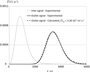
The RTD response to a Dirac-like injection is given by the distri-bution function EðtÞ which is a normalized function of the average concentration over the analyzed cross-section (Fig. 4).

EðtÞ ¼R1hCiðtÞ

0hCiðtÞdt

ð29Þ

With a perfect Dirac signal at the reactor inlet, the axial disper-sion coefficient can be obtained by fitting with an analytical solu-tion provided by a convecsolu-tion-dispersion model. In this work, in order to take into account the imperfection of the inlet signal, it is chosen to solve the 1D convection-dispersion equation in terms of distribution function (Eq.(30)) using the experimental inlet sig-nal as boundary condition.

@E @tþ huzi @E @z# @ @z Dax @E @z " # ¼ 0 ð30Þ

At initial time, there is no tracer in the channel: E = 0 at t = 0. The boundary conditions are as follows:

- experimental signal at the capillary inlet: EðtÞ = Einlet;expðtÞ at z = 0;

- conservation of the flux at the channel outlet:@E

@z= 0 at z = L. -6.E-06 -4.E-06 -2.E-06 0.E+00 2.E-06 0 5000 10000 15000 20000 0.E+00 1.E-07 2.E-07 3.E-07 4.E-07 0 5000 10000 15000 20000

(m

2

_.s

-1

₎

s

D

t

(a)

(s)

(m

2

_.s

-1

₎

s

D

t

(b)

(s)

Fig. 2.Impact of the injection function of the tracer on the spatial dispersion coefficient: (a) with a Dirac function and (b) with Eq.(27). The simulations are carried out in a straight circular channel (dH= 2 mm, L = 0.27 m, huzi = 10#4m"s#1).

Fluidoutput Light emiCer

Spectrophotometer

Syringe pump

Op+cal fiber

Eq.(30) is solved using Comsol Multiphysics 4.3b. Dax is set equal to the coefficient obtained with the numerical method, i.e. Dax= 3.30 " 10#7m2"s#1. As it can be seen in Fig. 4, such a value allows a very good prediction of the experimental outlet signal.

4. Application to millimetric wavy channels 4.1. Channel geometry

Wavy channels with different square and rectangular cross-sections have been considered in this study. Millimetric wavy channels are notably used in heat exchangers-reactors developed by the Laboratoire de Génie Chimique (LGC - Toulouse, France). These devices were built in different materials such as silicon car-bide (built by Boostec company - France) or stainless steel (built by the Commissariat à l’énergie atomique et aux énergies alternatives, CEA - France). This pattern allows an enhancement of mixing, mass and heat transfer compared to straight channels with reasonable pressure drops (Anxionnaz-Minvielle et al., 2013). Indeed, despite laminar flow, the bends generate vortices, so-called Dean vortices (Dean, 1928), that promote species transport from the walls to the channel center. This device has been successfully used to carry out exothermic reactions (Elgue et al., 2012; Despènes et al., 2012; Di Miceli Raimondi et al., 2015).

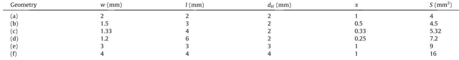
The channel geometry consists in a periodic zigzag (Fig. 5). The straight length between two bends is Ls= 10 mm. The bends are characterized by an angle of 90" and a curvature radius at the cen-ter of the channel of Rc= 4 mm. The total developed length of the channel simulated is L = 0.27 m which corresponds to 16 straight lengths and bends. Different cross-sections have been considered function of the channel width w and depth l as shown inTable 1.

This allows to study the sensitivity of axial dispersion to the hydraulic diameter (dH¼ 2w " l=ðw þ lÞ) and to the aspect ratio of the section (

a

¼ w=l;

a

¼ 1 for a square section). For rectangular cross-sections, it has to be noted that deep channels have been considered in the present study because of the bend curvature. Deep channels are more flexible in terms of design compared to wide channels since lower curvature radii can be obtained, favor-ing the appearance of Dean vortices.

4.2. Structure and size of the mesh grid

For simple geometries, cartesian meshes should be used in sim-ulations because they minimize numerical diffusion (Hirsch, 2007). In this work, because of the bends, a structured mesh adjusted at the curves or a tetrahedral mesh must be used. A structured mesh generates cells of very different sizes. Their volume decreases from the external side to the internal side of the bends. Very small cells may affect the convergence of the simulations and very small steps in time are so required to solve the equations, leading to highly time consuming simulations. Therefore, despite a loss in the simu-lation accuracy, a tetrahedral mesh is preferred to a structured mesh. However, it appeared that the axial dispersion coefficient estimated with Eq. (23) was fluctuating according to time with such an unstructured mesh. This fluctuation is mainly due to the need to interpolate the velocity and the concentration fields to cal-culate the terms averaged on the channel cross-section. Indeed the calculation nodes in the tetrahedral mesh do not fit with the chan-nel cross-section. Therefore, a structured mesh (cubic mesh) is used locally around the section where the axial dispersion coeffi-cient is calculated as illustrated inFig. 6.

As it can be seen inFig. 6, for each mesh, the size of the cells over a cross-section is uniform. Indeed, CFD simulations are gener-ally carried out with refined meshes near the wall where the shear rate is maximal. Nevertheless, numerical diffusion increases with velocity: its impact is thus more significant in the zone where velocity is higher i.e. around the channel center and can be reduced by decreasing the mesh size. For these reasons, uniform meshes have been used.

The sensitivity of the axial dispersion coefficient to the size of both tetrahedral and cubic meshes was studied. As noted before, numerical diffusion has a major impact at the highest fluid veloc-ity: the sensitivity study was carried out for the higher velocity condition for each channel geometry. The adequate sizes of the meshes (i.e. simulation results are mesh-independent) for the dif-ferent studied cases are given inTable 2.

4.3. Results

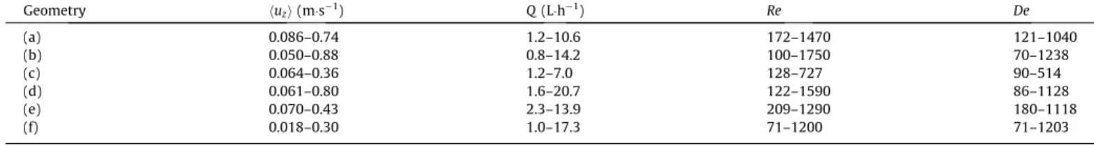
Axial dispersion coefficients are estimated using the numerical methodology previously described. The ranges of average velocity simulated for each reactor geometry are given inTable 3, as well as the ranges of flow rate, Reynolds number and Dean number (Eq.(31)). De ¼ Re ffiffiffiffiffiffi dH Rc s ð31Þ

The impact of the geometrical parameters (hydraulic diameter and aspect ratio of the cross-section) on axial dispersion is studied. 4.3.1. Effect of hydraulic diameter

The geometries with a square cross-section are considered. Fig. 7shows that axial dispersion coefficient increases with veloc-ity, and so with flow rate, according to a linear trend. At constant average velocity, it appears that axial dispersion coefficient varies slightly in function of the hydraulic diameter (Fig. 7(a)). Axial

L

s

w

l

Fig. 5.Wavy channel geometry.

(s-1₎

)

(t

E

(s)

t

0 0.0004 0.0008 0.0012 6000 4000 2000 0

Inlet signal - Experimental

Outlet signal - Experimental

Outlet signal - Calculated, Dax = 3.3e-7 m2.s-1= 3.30·10-7_m2_.s-1

ax

D

dispersion phenomenon significantly depends on the characteristic time to tangentially transport the tracer compared to the charac-teristic time to axially transport the tracer. At constant velocity in laminar flow, this last time is the same for the three geometries. However, time to tangentially transport the tracer is influenced by the hydraulic diameter: (i) in a negative way through the charac-teristic length of a tangential recirculation loop in a Dean vortex which increases with dhand (ii) in a positive way through Dean number which increases with dhimplying more important tangen-tial velocities. The weak influence of dhon Daxmay be due to the competition between these two contradictory effects.

Since axial dispersion coefficient varies slightly in function of the hydraulic diameter at constant velocity, it obviously signifi-cantly decreases with the hydraulic diameter at constant flow rate due to the impact of this dimension on the cross-sectional area (Fig. 7(b)). These two figures illustrate the impact of different scale-up strategies on axial dispersion, for instance if the hydraulic diameter is increased to increase the flow rate (constant mean velocity) or to decrease the pressure drop (constant flow rate).

4.3.2. Effect of cross-sectional aspect ratio

The geometries with different cross-sectional aspect ratio for a constant hydraulic diameter of 2 mm are considered. It can be seen inFig. 8that axial dispersion coefficient increases with velocity, and so with flow rate. It appears that at constant average velocity, axial dispersion coefficient increases when the aspect ratio decreases with a sharp increase for

a

- 0.33. Indeed, two sets of data can be distinguished: geometries (a) and (b) give similar results in terms of axial dispersion coefficient; the same observa-tion can be made for geometries (c) and (d) but with significantly

higher values of axial dispersion coefficient than for the two other geometries.Aubin et al. (2009)compared axial dispersion coeffi-cients in straight microchannels of square and rectangular cross-section. As in the present study, they observed a critical value of aspect ratio, approximately 0.3, from which a sharp decrease in the axial dispersion coefficient was observed. However, unlike in wavy channels, they showed that rectangular channels generate less axial dispersion than square channels. Wörner (2010) observed the same tendency. It implicitly means that the wavy configuration leads to opposite trends as regards axial dispersion in comparison with straight channels. These contradictory tenden-cies can be explained as follows. In laminar flow, at constant Rey-nolds number, axial dispersion effects can be reduced if the channel geometry allows to reduce the characteristic time to tan-gentially transport the tracer. In straight channel, this transport is ensured by molecular diffusion which is faster in rectangular channels than in square ones because the characteristic length of tangential diffusion is reduced (shortest dimension over the cross-section). Moreover, even when diffusive effects are negligi-ble,Wörner (2010)argued that the ratio of the maximal velocity to the mean velocity is lower in rectangular channels than in square channels leading to a reduction of the axial dispersion of the tracer. Unlike straight channels, tangential transport by advec-tion occurs in wavy channels due to Dean vortices. The ratio of the cross-section where tangential advection is efficient to the total cross-section is probably higher in square channels than in rectan-gular ones. A possible explanation lies in the increase of the wetted perimeter at constant hydraulic diameter (where velocity is zero) with the decrease of the aspect ratio.

4.3.3. Modelling of axial dispersion

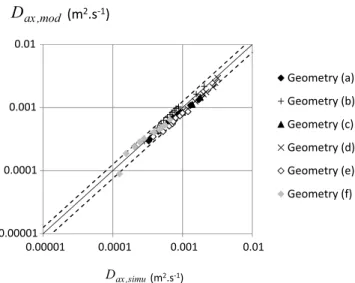
In order to express the influence of the velocity, the hydraulic diameter and the cross-sectional aspect ratio on the axial disper-sion coefficient, a correlation is proposed obtained from the simu-lation results presented inFig. 7andFig. 8. It is expressed in terms of the dimensionless quantity Dax=ðhuzidHÞ – which corresponds to the inverse of a Péclet number – as function of Reynolds number, Dean number and the cross-sectional aspect ratio:

Dax

huzidH¼ 4:5 " Re

1:38_De#1:68

a

#0:53 _ð32Þ

Fig. 9shows that Eq.(32)reasonably fits the simulation results, with an average relative error of 13.4% and a maximal relative error of 29%. The ranges of the parameters considered to establish the correlation are as follows: dH= 2–4 mm;

a

= 0.25–1; Re = 70–1 600. The effect of the physicochemical properties of the fluid has not been investigated.

Table 1

Characteristics of the wavy channels.

Geometry w (mm) l (mm) dH(mm) a S (mm2) (a) 2 2 2 1 4 (b) 1.5 3 2 0.5 4.5 (c) 1.33 4 2 0.33 5.32 (d) 1.2 6 2 0.25 7.2 (e) 3 3 3 1 9 (f) 4 4 4 1 16

Sec+on for D

ax

calcula+on

Flow direc+on

Fig. 6.Hybrid mesh grid used in the numerical method.

Table 2

Size of the meshes.

Geometry (a) (b) (c) (d) (e) (f)

dtetrahdral(lm) 150 200 100 200 75 200

Eq. (32) can be compared to Eqs. (3) and (5) that give the dimensionless quantity Dax=ðhuzidHÞ in a straight tube in laminar flow and turbulent flow respectively. In laminar flow, it can be seen that this quantity increases with the mean velocity. The opposite trend is observed in turbulent flow such as in the wavy channels despite laminar flow conditions. Indeed it is observed that Dax=ðhuzidHÞ is proportional to huzi#0:3 in the present study.

4.3.4. Comparison with experimental results

RTD experiments have been carried out in a PMMA (poly(methyl methacrylate)) mock-up where a wavy channel cor-responding to geometry (a) is engraved. The experimental method is analogous to the one described in Section3.3.1. The mean veloc-ity range studied is 0.086–0.39 m"s#1_{. The channel length is the} same than in the simulation work – L = 0.27 m – resulting in

Table 3

Range of the simulated operating conditions.

Geometry huzi (m"s#1) Q (L"h#1) Re De (a) 0.086–0.74 1.2–10.6 172–1470 121–1040 (b) 0.050–0.88 0.8–14.2 100–1750 70–1238 (c) 0.064–0.36 1.2–7.0 128–727 90–514 (d) 0.061–0.80 1.6–20.7 122–1590 86–1128 (e) 0.070–0.43 2.3–13.9 209–1290 180–1118 (f) 0.018–0.30 1.0–17.3 71–1200 71–1203 0.0E+00 5.0E-04 1.0E-03 1.5E-03 2.0E-03 0 0.2 0.4 0.6 0.8 0.0E+00 5.0E-04 1.0E-03 1.5E-03 2.0E-03 0 5 10 15 20

(m

2

_.s

-1

₎

ax

D

(m.s-1₎ z

u

Geometry (a)

Geometry (e)

Geometry (f)

(m

2

_.s

-1

₎

ax

D

(L.h-1₎

Q

, d

H

= 2 mm

, d

H

= 3 mm

, d

_H

= 4 mm

(a)

(b)

Fig. 7.Axial dispersion coefficient vs (a) average velocity and (b) flow rate. Impact of the hydraulic diameter (a= 1).

(m

2

_.s

-1

₎

ax

D

(m.s-1₎ z

u

(m

2

_.s

-1

₎

ax

D

(L.h-1₎

Q

(a)

(b)

0.0E+00 5.0E-04 1.0E-03 1.5E-03 2.0E-03 2.5E-03 3.0E-03 3.5E-03 0 0.2 0.4 0.6 0.8 1 0.0E+00 5.0E-04 1.0E-03 1.5E-03 2.0E-03 2.5E-03 3.0E-03 3.5E-03 0 5 10 15 20 25

Geometry (a)

Geometry (b)

Geometry (c)

Geometry (d)

,

α

= 1

,

α

= 0.5

,

α

_{= 0.33}

,

α

= 0.25

residence times between 0.7 s and 3.1 s.Fig. 10allows to compare the experimental results and those obtained thanks to the numer-ical method.

It can be observed that the numerical method allows to repro-duce the global trend obtained with the experiments despite a sig-nificant uncertainty on the experimental points. This uncertainty is due to the perturbation of the flow at the injection of the tracer and the importance of the noise on the entrance and the outlet absor-bance signals. This noise is related to the high frequency of acqui-sition (30 ms between each absorbance measurement) required to have a sufficient number of points on the RTD curves regarding the low residence times in the channel. These results illustrate the dif-ficulty to accurately characterize axial dispersion in short resi-dence time devices.

5. Conclusion

An original method for the characterization of axial dispersion in microreactors is presented. It is based on simulations using a

CFD software. Comsol Multiphysics is used to solve continuity equation and Navier-Stokes equation to calculate the velocity field in the reactor, and the transport equation to predict the concentra-tion field in tracer. These data allow the estimaconcentra-tion of the axial dis-persion coefficient considering an incompressible fluid and a reactor with a constant cross-section. In the present work, the method has been used under laminar flow regime and validated by comparison with an experimental result obtained from a RTD experiment in a circular straight capillary. This method can also be used in turbulent flow regime (Talvy et al., 2007) as long as an adequate turbulence model is used in the simulations.

The numerical method is applied to wavy millimetric channels with square and rectangular cross-section. Hydraulic diameters of 2–4 mm have been considered. Wavy channels are notably used in intensified compact reactors since the bends generate vortices that enhance mixing despite laminar flow and so heat and mass trans-fer. The study aims at investigating the impact of the cross-sectional aspect ratio of the channel and its hydraulic diameter on axial dispersion. It has been shown that square wavy channels generate less axial dispersion that rectangular ones, with a signif-icant increase of axial dispersion coefficient at constant average velocity when the channel depth is more than three times higher than its width. Finally, in square channel, it appears that axial dis-persion coefficient varies slightly in function of the hydraulic diam-eter at constant average velocity. These results have been expressed in terms of a correlation using dimensionless quantities that can be used then to predict the pertinent strategy to modify the operating conditions or the channel design in order to reduce axial dispersion phenomenon. However this correlation must be validated with other materials than water in order to study the influence of the fluid physicochemical properties on axial disper-sion, and with geometries designed with various curvature radii and straight lengths between two bends to be more generic. Acknowledgements

This work has been supported by the ANR (Agence Nationale de la Recherche), France: Project ANR PROCIP, ANR-2010-CD2I-013-01. The experimental facility was supported by: the FNADT, Grand Toulouse, Prefecture Midi-Pyrenees and FEDER fundings.

References

Adeosun, J.T., Lawal, A., 2009. Numerical and experimental studies of mixing characteristics in a T-junction microchannel using residence-time distribution. Chem. Eng. Sci. 64, 2422–2432.http://dx.doi.org/10.1016/j.ces.2009.02.013. Ajdari, A., Bontoux, N., Stone, H.A., 2006. Hydrodynamic dispersion in shallow

microchannels: the effect of cross-sectional shape. Anal. Chem. 78, 387–392.

http://dx.doi.org/10.1021/ac0508651.

Amador, C., Wenn, D., Shaw, J., Gavriilidis, A., Angeli, P., 2008. Design of a mesh microreactor for even flow distribution and narrow residence time distribution. Chem. Eng. J. 135, S259–S269.http://dx.doi.org/10.1016/j.cej.2007.07.021. Anxionnaz-Minvielle, Z., Cabassud, M., Gourdon, C., Tochon, P., 2013. Influence of

the meandering channel geometry on the thermo-hydraulic performances of an intensified heat exchanger/reactor. Chem. Eng. Process. Process Intensif. 73, 67– 80.http://dx.doi.org/10.1016/j.cep.2013.06.012.

Anxionnaz, Z., Cabassud, M., Gourdon, C., Tochon, P., 2008. Heat exchanger/reactors (HEX reactors): concepts, technologies: state-of-the-art. Chem. Eng. Process. Process Intensif. 47, 2029–2050.http://dx.doi.org/10.1016/j.cep.2008.06.012. Aris, R., 1956. On the dispersion of a solute in a fluid flowing through a tube. Proc. R.

Soc. Lond. Math. Phys. Eng. Sci. 235, 67–77. http://dx.doi.org/10.1098/ rspa.1956.0065.

Aubin, J., Prat, L., Xuereb, C., Gourdon, C., 2009. Effect of microchannel aspect ratio on residence time distributions and the axial dispersion coefficient. Chem. Eng. Process. Process Intensif. 48, 554–559. http://dx.doi.org/10.1016/ j.cep.2008.08.004.

Bai, H., Stephenson, A., Jimenez, J., Jewell, D., Gillis, P., 2008. Modeling flow and residence time distribution in an industrial-scale reactor with a plunging jet inlet and optional agitation. Chem. Eng. Res. Des. 86, 1462–1476.http://dx.doi. org/10.1016/j.cherd.2008.08.012.

Blet, V., Berne, P., Legoupil, S., Vitart, X., 2000. Radioactive tracing as aid for diagnosing chemical reactors. Oil Gas Sci. Technol. 55, 171–183.

(m

2

_.s

-1

₎

ax

D

(m.s-1₎ z

u

0.0E+00 5.0E-04 1.0E-03 1.5E-03 2.0E-03 0 0.2 0.4 0.6 0.8

Simula+on

Experiment

Fig. 10.Comparison between axial dispersion coefficients obtained by simulations and by RTD experiments in geometry (a).

(m

2

_.s

-1

₎

mod , ax

D

(m2_.s-1₎ simu , ax

D

0.00001 0.0001 0.001 0.01 0.00001 0.0001 0.001 0.01 Geometry (a) Geometry (b) Geometry (c) Geometry (d) Geometry (e) Geometry (f)

Fig. 9.Comparison between axial dispersion coefficients obtained by simulations and calculated by the correlation given by Eq.(32). Dashed lines correspond to 25% of relative error.

Borroto, J.I., Domı´ nguez, J., Griffith, J., Fick, M., Leclerc, J.P., 2003. Technetium-99m as a tracer for the liquid RTD measurement in opaque anaerobic digester: application in a sugar wastewater treatment plant. Chem. Eng. Process. Process Intensif. 42, 857–865.http://dx.doi.org/10.1016/S0255-2701(02)00109-5. Boskovic, D., Loebbecke, S., 2008. Modelling of the residence time distribution in

micromixers. Chem. Eng. J. 135, S138–S146. http://dx.doi.org/10.1016/j. cej.2007.07.058.

Castelain, C., Berger, D., Legentilhomme, P., Mokrani, A., Peerhossaini, H., 2000. Experimental and numerical characterisation of mixing in a steady spatially chaotic flow by means of residence time distribution measurements. Int. J. Heat Mass Transf. 43, 3687–3700.http://dx.doi.org/10.1016/S0017-9310 (99)00363-4.

Dean, W.R., 1928. Fluid motion in a curved channel. Proc. R. Soc. Lond. Math. Phys. Eng. Sci. 121, 402–420.http://dx.doi.org/10.1098/rspa.1928.0205.

Despènes, L., Elgue, S., Gourdon, C., Cabassud, M., 2012. Impact of the material on the thermal behaviour of heat exchangers-reactors. Chem. Eng. Process. Process Intensif. 52, 102–111.http://dx.doi.org/10.1016/j.cep.2011.11.005.

Di Miceli Raimondi, N., Olivier-Maget, N., Gabas, N., Cabassud, M., Gourdon, C., 2015. Safety enhancement by transposition of the nitration of toluene from semi-batch reactor to continuous intensified heat exchanger reactor. Chem. Eng. Res. Des. 94, 182–193. http://dx.doi.org/10.1016/j.cherd. 2014.07.029.

Elgue, S., Conté, A., Gourdon, C., Bastard, Y., 2012. Direct fluorination. Chem. Today, 30.

Elias, Y., Rudolf von Rohr, P., 2016. Axial dispersion, pressure drop and mass transfer comparison of small-scale structured reaction devices for hydrogenations. Chem. Eng. Process. Process Intensif. 106, 1–12. http://dx.doi.org/10.1016/ j.cep.2015.11.017.

Günther, M., Schneider, S., Wagner, J., Gorges, R., Henkel, T., Kielpinski, M., Albert, J., Bierbaum, R., Köhler, J.M., 2004. Characterisation of residence time and residence time distribution in chip reactors with modular arrangements by integrated optical detection. Chem. Eng. J. 101, 373–378.http://dx.doi.org/ 10.1016/j.cej.2003.10.019.

Gutierrez, C.G.C.C., Dias, E.F.T.S., Gut, J.A.W., 2010. Residence time distribution in holding tubes using generalized convection model and numerical convolution for non-ideal tracer detection. J. Food Eng. 98, 248–256.http://dx.doi.org/ 10.1016/j.jfoodeng.2010.01.004.

Habchi, C., Lemenand, T., Della Valle, D., Peerhossaini, H., 2010. Turbulent mixing and residence time distribution in novel multifunctional heat exchangers– reactors. Chem. Eng. Process. Process Intensif. 49, 1066–1075.http://dx.doi.org/ 10.1016/j.cep.2010.08.007.

Häfeli, R., Hutter, C., Damsohn, M., Prasser, H.-M., Rudolf von Rohr, P., 2013. Dispersion in fully developed flow through regular porous structures: experiments with wire-mesh sensors. Chem. Eng. Process. Process Intensif. 69, 104–111.http://dx.doi.org/10.1016/j.cep.2013.03.006.

Hirsch, C., 2007. Chapter 6 - structured and unstructured grid properties. In: Hirsch, C. (Ed.), Numerical Computation of Internal and External Flows. second ed. Butterworth-Heinemann, Oxford, pp. 249–277.

Kolar, Z., Thyn, J., Martens, W., Boelens, G., Korving, A., 1987. The measurement of gas residence time distribution in a pressurized fluidized-bed combustor using41Ar as radiotracer. Int. J. Rad. Appl. Instrum. 38, 117–122.http://dx.doi. org/10.1016/0883-2889(87)90006-2.

Kurt, S.K., Gelhausen, M.G., Kockmann, N., 2015. Axial dispersion and heat transfer in a milli/microstructured coiled flow inverter for narrow residence time distribution at laminar flow. Chem. Eng. Technol. 38, 1122–1130.http://dx.doi. org/10.1002/ceat.201400515.

Lelinski, D., Allen, J., Redden, L., Weber, A., 2002. Analysis of the residence time distribution in large flotation machines. Miner. Eng. 15, 499–505.http://dx.doi. org/10.1016/S0892-6875(02)00070-5.

Le Moullec, Y., Potier, O., Gentric, C., Leclerc, J.P., 2008. Flow field and residence time distribution simulation of a cross-flow gas–liquid wastewater treatment reactor using CFD. Chem. Eng. Sci. 63, 2436–2449. http://dx.doi.org/10.1016/j. ces.2008.01.029.

Levenspiel, O., 1999. Chemical Reaction Engineering. Wiley, New York. Lohse, S., Kohnen, B.T., Janasek, D., Dittrich, P.S., Franzke, J., Agar, D.W., 2008. A novel

method for determining residence time distribution in intricately structured microreactors. Lab Chip 8, 431.http://dx.doi.org/10.1039/b714190d. Lutze, P., Gani, R., Woodley, J.M., 2010. Process intensification: a perspective on

process synthesis. Chem. Eng. Process. Process Intensif. 49, 547–558.http://dx. doi.org/10.1016/j.cep.2010.05.002.

Mohammadi, S., Boodhoo, K.V.K., 2012. Online conductivity measurement of residence time distribution of thin film flow in the spinning disc reactor. Chem. Eng. J. 207–208, 885–894.http://dx.doi.org/10.1016/j.cej.2012.07.120. Moreau, M., Di Miceli Raimondi, N., Le Sauze, N., Cabassud, M., Gourdon, C., 2015.

Pressure drop and axial dispersion in industrial millistructured heat exchange reactors. Chem. Eng. Process. Process Intensif. 95, 54–62. http://dx.doi.org/ 10.1016/j.cep.2015.05.009.

Nagy, K.D., Shen, B., Jamison, T.F., Jensen, K.F., 2012. Mixing and dispersion in small-scale flow systems. Org. Process Res. Dev. 16, 976–981. http://dx.doi.org/ 10.1021/op200349f.

Nikacˇevic´, N.M., Huesman, A.E.M., Van den Hof, P.M.J., Stankiewicz, A.I., 2012. Opportunities and challenges for process control in process intensification. Chem. Eng. Process. Process Intensif. 52, 1–15. http://dx.doi.org/10.1016/ j.cep.2011.11.006.

Sahle-Demessie, E., Bekele, S., Pillai, U.R., 2003. Residence time distribution of fluids in stirred annular photoreactor. Catal. Today 88, 61–72. http://dx.doi.org/ 10.1016/j.cattod.2003.08.009.

Sancho, M.F., Rao, M.A., 1992. Residence time distribution in a holding tube. J. Food Eng. 15, 1–19.http://dx.doi.org/10.1016/0260-8774(92)90037-7.

Squires, T.M., Quake, S.R., 2005. Microfluidics: fluid physics at the nanoliter scale. Rev. Mod. Phys. 77, 977.

Talvy, S., Cockx, A., Liné, A., 2007. Modeling hydrodynamics of gas–liquid airlift reactor. AIChE J. 53, 335–353.http://dx.doi.org/10.1002/aic.11078.

Taylor, G., 1953. Dispersion of soluble matter in solvent flowing slowly through a tube. Proc. R. Soc. Lond. Math. Phys. Eng. Sci. 219, 186–203.http://dx.doi.org/ 10.1098/rspa.1953.0139.

Trambouze, P., Euzen, J.-P., 2004. Chemical Reactors: From Design to Operation. Institut français du pétrole publications, Editions Technip, Paris.

Van Gerven, T., Stankiewicz, A., 2009. Structure, energy, synergy, time - the fundamentals of process intensification. Ind. Eng. Chem. Res. 48, 2465–2474.

http://dx.doi.org/10.1021/ie801501y.

Wörner, M., 2010. Approximate residence time distribution of fully develop laminar flow in a straight rectangular channel. Chem. Eng. Sci. 65, 3499–3507.http://dx. doi.org/10.1016/j.ces.2010.02.047.