Can We Identify the Fed's Preferences?

HAL Id: halshs-01549908

https://halshs.archives-ouvertes.fr/halshs-01549908v3

Preprint submitted on 4 Dec 2017

HAL is a multi-disciplinary open access

archive for the deposit and dissemination of sci-entific research documents, whether they are pub-lished or not. The documents may come from teaching and research institutions in France or abroad, or from public or private research centers.

L’archive ouverte pluridisciplinaire HAL, est destinée au dépôt et à la diffusion de documents scientifiques de niveau recherche, publiés ou non, émanant des établissements d’enseignement et de recherche français ou étrangers, des laboratoires publics ou privés.

Can We Identify the Fed’s Preferences?

Jean-Bernard Chatelain, Kirsten Ralf

To cite this version:

Jean-Bernard Chatelain, Kirsten Ralf. Can We Identify the Fed’s Preferences?. 2017. �halshs-01549908v3�

WORKING PAPER N° 2017 – 25

Can we Identify the Fed’s Preferences?

Kirsten Ralf

JEL Codes: C61, C62, E31, E52, E58

Keywords: Ramsey optimal policy, zero-credibility policy, Identification, Central bank preferences, New-Keynesian Phillips curve, Working capital channel

P

-

S

E

48, BD JOURDAN – E.N.S. – 75014 PARIS

TÉL. : 33(0) 1 80 52 16 00=

www.pse.ens.fr

Can we Identify the Fed’s Preferences?

Jean-Bernard Chatelain

Kirsten Ralf

December 2, 2017

Abstract

Using US data, we estimate optimal policy with a probability below one that the Fed reneges on its commitment ("limited credibility") versus discretionary policy where the Fed reneges on its commitment at all periods with a probability equal to one ("zero credibility"). The transmission mechanism is the new-Keynesian Phillips curve with auto-correlated cost-push shock. It includes the labor cost channel or the working capital channel. Discretion with zero credibility of the Fed is rejected. The working capital channel …ts the data before Volcker’s mandate. The labor cost channel …ts the data since Volcker’s mandate.

JEL classi…cation numbers: C61, C62, E31, E52, E58.

Keywords: Ramsey optimal policy, zero-credibility policy, Identi…cation, Central bank preferences, New-Keynesian Phillips curve,

Working capital channel.

1

Introduction

Can we test if the Fed follows Ramsey optimal policy under the limited credibility of quasi-commitment with a non-zero probability to commit (Debortoli and Nunes (2014), Schaumburg and Tambalotti (2007), Roberts (1987)) versus the Fed follows a policy with a complete lack of credibility with a zero probability to commit (Oudiz and Sachs (1985))? Are the Fed’s preferences facing the same identi…cation problem as Taylor rule parameters for both types of policies? Cochrane (2011) found that the simple Taylor rule parameters are not identi…ed in new-Keynesian models including forward-looking in‡ation, but only the auto-correlation parameters of non-observable shocks.

Beginning with Simon (1956) certainty equivalence property of the linear quadratic regulator, the quadratic loss function describing policy-maker’s preferences is used for modelling stabilization policy (Duarte (2009)). It took more than two decades for the estimation of Fed’s preferences to begin with Salemi (1995), using inverse control (Salemi (2010)). Salemi (1995) took into account two structural breaks (1970-1, 1979-10) for three monetary policy regime during the period 1947-1992 using monthly data. Salemi (1995) includes a careful investigation of identi…cation issues when the monetary policy trans-mission mechanism is a backward-looking vector auto-regressive (VAR) model. These

We thank our discussants in conferences Robert Kollman, Sumudu Kankanamge, Gregory Levieuge and Efrem Castelnuovo, as well as Georges Overton for very helpful insights.

y_{Paris School of Economics, Université Paris 1 Pantheon Sorbonne, PjSE, 48 Boulevard Jourdan,}

75014 Paris. Email: jean-bernard.chatelain@univ-paris1.fr

identi…cation issues are the same for Ramsey optimal policy under quasi-commitment (Debortoli and Nunes (2014)) with forward-looking variables, besides the optimal initial jump anchoring forward-looking variables (Ljungqvist and Sargent (2012)).

Following Salemi (1995), there are more than twenty papers estimating Fed’s prefer-ences since the 1960’s with a structural break since the 1980’s (Volcker-Greenspan period) assuming in‡ation is a predetermined variable or a forward-looking variable, assuming the acceleration Phillips curve or new-Keynesian Phillips curve as a monetary policy transmission mechanism: e.g. Cechetti and Ehrmann (2002), Ozlale (2003), Favero and Rovelli (2003), Castelnuovo and Surico (2004), Castelnuovo (2006), Soderstrom et al. (2005), Juillard et al. (2006), Salemi (2006), Kara (2007), Adjemian and Devulder (2011), Adolfson et al. (2011), Ilbas (2012), Levieuge and Lucotte (2014), Paez-Farrell (2015), Debortoli and Lakdawala (2016) and many others.

Ramsey optimal policy including the probability to re-optimize each period is men-tioned "stochastic replanning" (Roberds (1987)), "quasi commitment" (Schaumburg and Tambalotti (2007), Kara (2007)) or "loose commitment" (Debortoli and Nunes (2010)). This assumption is observationally equivalent to Chari and Kehoe (1990) optimal pol-icy under sustainable plans facing a punishment threat at a given horizon T in case of deviation of an Ramsey optimal policy plan (Fujiwara, Kam, Sunakawa (2016)).

We estimate Debortoli and Nunes (2014) and Schaumburg and Tambalotti (2007) quasi commitment model, where the transmission mechanism is the new-Keynesian Phillips curve with an auto-regressive cost-push shock. These empirical results can be compared to estimations of the new-Keynesian Phillips curve (Mavroeidis et al. (2014)). We avoid the Lucas’critique taking into account the endogeneity of the policy instruments due to a feedback policy rule. We also estimate that case of the working capital channel with interest smoothing in the Fed’s loss function. In this case, the model …ts data as well as a non-structural VAR for the pre-Volcker period. We test Ramsey versus zero-credibility policy. Assuming the minimal number of lags for the transmission mechanism, this paper makes progress in these …ve directions:

(1) We disclose the estimates of the reduced form stable eigenvalues of the estimated VAR for Ramsey versus zero-credibility and check Blanchard and Kahn (1980) determi-nacy condition. The estimations should not correspond to the same number of stable eigenvalues for both models. Söderlind (1999) algorithm provides no hints on checking the number of stable eigenvalues for Ramsey versus zero-credibility policy.

(2) We disclose the conditions for the exact identi…cation of parameters for each model. (3) We test the signs restrictions of reduced form policy rule parameters.

(4) We test the misspeci…cation of each models, using for example Durbin (1970) test. (5) We compare both estimations with the estimations of a non-structural vector auto-regressive model.

Section 2 presents our estimation methods of Ramsey optimal policy and zero-credibility policy. Section 3 details speci…cation tests of zero-credibility versus Ramsey optimal pol-icy. Section 4 presents estimations on US data during 1960-2006 for a labor cost channel and section 5 for a cost of working capital channel. The last section concludes.

2

Ramsey versus Zero-credibility Monetary Policy

2.1

Monetary Policy Transmission Mechanism Including or not

the Cost of Working Capital

The reference new-Keynesian Phillips curve is the monetary policy transmission mecha-nism:

t= Et[ t+1] + xt+ ut where > 0, 0 < < 1 (1)

where xt represents the welfare-relevant output gap, i.e. the deviation between (log)

output and its e¢ cient level. tdenotes the rate of in‡ation between periods t 1and t.

ut denotes a cost-push shock. denotes the discount factor. Et denotes the expectation

operator. The cost push shock ut includes an exogenous auto-regressive component:

ut= ut 1+ "u;t where 0 < < 1 and "u;t i.i.d. normal N 0; u2 (2)

where denotes the auto-correlation parameter and "tis identically and independently

distributed (i.i.d.) according to a normal distribution with constant variance 2 u.

The reduced-form parameter (denoted ) of the slope of the new-Keynesian Phillips curve relates in‡ation to marginal cost or to the output gap. It depends on four structural parameters: the representative household discount factor , the household’s elasticity of substitution between each di¤erentiated goods ", the measure of decreasing returns to scale of labor in the production functions of the …rms , and the proportion of …rms who do not reset their price each period (Gali (2015), chapter 3):

( ; "; ; ) = (1 ) (1 ) (1 )

(1 + "):

In the new-Keynesian model, labor is assumed to be the only input in the production function. The cost of capital channel of monetary policy is ruled out by assumption. Christiano, Trabandt and Walentin (2010) assume that labor cost is …nanced by working capital. The marginal cost in the new-Keynesian Phillips curve is then a linear combi-nation of labor and capital cost (Christiano, Trabandt and Walentin (2010), equation 35):

(1 + ) xt+

(1 ) + it (3)

We estimate two polar cases. When material inputs are not used in production ( = 1) and when no labor cost is …nanced by working capital ( = 0), the cost of labor is the only cost taken into account and the output gap is the policy instrument. When material inputs are all used in production ( = 0) and when all labor cost is …nanced by working capital ( = 1), the cost of capital is the only cost taken into account with a slope of

the new-Keynesian Phillips curve denoted i. Then, the Federal funds rate is the policy

instrument with an interest smoothing parameter i for the Fed’s preferences.

2.2

Monetary Policy Regimes and Central Bank Behavior

In a monetary policy regime indexed by j, a policy maker has a period loss function

1 2(

2

smoothing term 1₂( 2

t + i;ji2t) for the cost of working capital model. Fed’s preferences

are represented by the relative cost x;j > 0 or i;j > 0 of changing its policy

instru-ment. A policy maker may re-optimize on each future period with exogenous probability 1 q strictly below one ("stochastic replanning" (Roberds, 1987), "quasi commitment" (Schaumburg and Tambalotti, 2007; Kara 2007) or "loose commitment" (Debortoli and Nunes, 2014)).

Following Schaumburg and Tambalotti (2007), we assume that the mandate to mini-mize the loss function is delegated to a sequence of policy makers with a commitment of random duration. The degree of credibility is modelled as if it is a change of policy-maker with a given probability of reneging commitment and re-optimizing optimal plans. The length of their tenure or "regime" depends on a sequence of exogenous i.i.d. Bernoulli signals f tgt 0 with Et[ t]t 0 = 1 q, with 0 < q < 1. If t = 1; a new policy maker

takes o¢ ce at the beginning of time t. Otherwise, the incumbent stays on. A higher probability q can be interpreted as a higher credibility. As seen below, this leads to use a "credibility adjusted" discount factor q in the policy maker’s optimal behavior.

Secondly, in this new monetary policy regime indexed by k, there may be a switch of

the transmission mechanism parameter (the slope of the Phillips curve) k including in

particular, a switch of the representative household’s elasticity of substitution between each di¤erentiated goods "k . Thirdly, the new policy maker may have new preferences x;k. If the policy maker is maximizing welfare, its preferences are given by the new values

of structural parameters of the transmission mechanism x;k = _"k_k (Gali (2015)). More

generally, and stepping beyond the welfare-theoretic justi…cation for (1), one can interpret

x as the weight attached by the central bank to deviations of output from its e¢ cient

level (relative to price stability) in its own loss function, which does not necessarily have to coincide with the household’s. Because structural parameters may change for a new regime k, long run equilibrium values may also change in the estimation.

Under regime j, policy plans solve the following problem (omitting subscript j for the

central bank preferences x, transmission mechanism parameter , the auto-correlation

of the cost-push shock and its variance of its disturbances "t):

Vjk(u0) = E0 t=+1_X t=0 ( q)t 1 2 2 t + xx2t + (1 q) V jk_(u t) (4) s.t. t = xt+ qEt t+1+ (1 q) Et t+1k + ut (Lagrange multiplier t+1) ut = ut 1+ "t,8t 2 N, u0 given.

The utility the central bank obtains is next period objectives change is denoted Vjk_.

Since when objectives change, the central bank loses its commitment, this value function depends on the policies of the alternative regime. In‡ation expectations are an average between two terms. The …rst term, with weight q is the in‡ation that would prevail under the current regime upon which there is commitment. The second term with weight

1 q is the in‡ation that would be implemented under the alternative regime, which is

taken as given by the current central bank. The key change is that the narrow range

of values for the discount factor _{2 [0:99; 1] for quarterly data (4% discount rate at}

most) is much wider for the "credibility weighted discount factor" of the policy maker:

q _{2 ]0; 1]. In what follows, the notation} will correspond to q, in order to simplify

q for the estimation.

2.3

VAR Representation of Ramsey optimal policy

Di¤erentiating the Lagrangian with respect to the policy instrument (output gap xt) and

to the policy target (in‡ation t) yields the …rst order conditions (see appendix 2): @L @ t = 0 : t+ t+1 t= 0 @L @xt = 0 : xxt t+1 = 0 ) xt= xt 1 x t xt= x t+1= x( t t)

that must hold for t = 1; 2; ::: The central bank’s Euler equation (_@@L

t = 0) links

recursively the future or current value of central bank’s policy instrument xtto its current

or past value xt 1, because of the central bank’s relative cost of changing her policy

instrument is strictly positive x > 0. This non-stationary Euler equation adds an

unstable eigenvalue in the central bank’s Hamiltonian system including three laws of motion of one forward variable (in‡ation t) and of two predetermined variables (ut; xt)

or (ut; t).

The natural boundary condition 0 = 0 minimizes the loss function with respect to

in‡ation at the initial date:

0 = 0 ) x 1 =

x

0 = 0 and 0 =

x

x0 6= 0

It predetermines the policy instrument which allows to anchor the forward-looking policy target (in‡ation). The in‡ation Euler equation corresponding to period 0 is not an e¤ective constraint for the central bank choosing its optimal plan in period 0. The former

commitment to the value of the policy instrument of the previous period x 1 is not an

e¤ective constraint. The policy instrument is predetermined at the value zero x 1 = 0

at the period preceding the commitment. Combining the two …rst order conditions to eliminate the Lagrange multipliers yields the optimal initial anchor of forward in‡ation

0 on the predetermined policy instrument x0.

Ljungqvist and Sargent (2012, chapter 19) seek the stationary equilibrium process us-ing the augmented discounted linear quadratic regulator solution of the Hamiltonian sys-tem (Anderson, Hansen, McGrattan and Sargent (1996)) as an intermediate step (Chate-lain and Ralf (2017) algorithm). The policy instrument is exactly correlated with private sectors variables:

xt= F t+ Fuut: (5)

We estimate three observationally equivalent estimations of Ramsey optimal policy structural VAR of the two observable variables (in‡ation and the policy instrument), using feasible generalized non-linear least squares for a system of equations (see appendix 2).

The …rst estimation estimates the two stable eigenvalues: the exogenous

auto-correlation of cost-push shock , the reduced form eigenvalue and the reduced from

policy rule parameter with respect to in‡ation F :

t+1 xt+1 = (1 ) 1 F ( 1) F + t xt + t+11 F "t+1 (6)

policy instrument. It does not appear into the disturbances, which are now white noise, a necessary condition for estimating a VAR. We assume an i.i.d. measurement error

t+1 in order to avoid the stochastic singularity of the perfect collinearity of the in‡ation

equation predicted by the Ramsey optimal policy theory (appendix 2). A high R2 _{for the}

in‡ation equation would signal that the variance of this measurement error is su¢ ciently small to remain close to the theoretical model.

t+1 xt+1 = 1 F _{(1 )}1 F 1 F 1 F _{1 F +}1 F 1 F ! t xt + t+11 F "t+1 (7) The second estimation estimates the two stable eigenvalues: the exogenous , the

reduced form eigenvalue and the ratio of two structural parameters x ₌ 1

" where " is

the household’s elasticity of substitution between each di¤erentiated goods, if the central bank maximizes the representative household welfare.

t+1 xt+1 = (1 ) (1 ) x x + t+1 xt+1 + t+11 F "t+1 (8)

The third estimation substitutes the reduced form stable eigenvalue by its

non-linear function of the three structural parameters ; x; in the above VAR of the second

estimation. = 1 F = 1 2 1 + 1 + 2 x s 1 4 1 + 1 2 x 2 1 q = (9)

This requires an identi…cation restriction that we set on the discount factor . We

estimate separately three structural parameters: the auto-correlation of the cost-push shock , the preference of the Fed x, and the slope of the new-Keynesian Phillips curve .

Only three structural parameters can be identi…ed: , , F or , , x _{or , ( q) ; ( q)}

for a given value of the discount factor q (see appendix 2):

( ) = 1 q

F ) x( ) = 1

1

F ( q) : (10)

If initial values of in‡ation and of the policy instrument (in deviation from their

equi-librium values) were perfectly measured at the date of commitment, the ratio x _would

be over-identi…ed by the optimal initial anchor of forward in‡ation on the predetermined policy instrument equation:

x

= 0

x0

: (11)

The semi-reduced form cost-push shock rule parameter Fu requires an identi…cation

restriction, for example, setting a value for (see appendix 2): Fu( ) =

1

1 F < 0: (12)

The standard error u of cost-push shock is computed using the standard error of

restriction, because it depends on Fu: u( ) = ";x Fu( ) = 1 F ";x: (13)

The standard error of the measurement of the in‡ation equation (which is

theo-retically predicted to be zero) and its covariance with the cost push shock x = Fu xu

are also available.

One identifying equation is missing in order to identify the remaining four structural

parameters ( x; ; ; u) and the negative feedback rule parameter Fu. We set an

iden-ti…cation restriction on the credibility weighted discount factor to a given values in the estimations.

For each regime, we estimate the slope of the Phillips curve j, the elasticity of

substitution between each di¤erentiated goods (_"1

j =

x;j

j ), the Fed’s preferences x;j, the

auto-correlation of the cost-push shock j and its variance u;j2 . We calibrate the two

parameters q. The measure of decreasing returns to scale of labor in the production

functions of the …rms and the proportion of …rms who do not reset their price each

period face an under-identi…cation problem detailed in the next section.

2.4

In…nite Horizon Zero-Credibility Policy

With quasi-commitment, the probability of not reneging commitment could be in…nitely small (near-zero credibility), but it remains strictly positive: for example, q = 10 7 _{> 0}

(Roberts (1987)) with q 2 ]0; 1]. Before Roberts (1987) stochastic replanning article, Oudiz and Sachs (1985) invented an in…nite horizon zero-credibility policy, which holds when the policy maker re-optimizes with certainty for all future periods. This forever complete lack of credibility corresponds to q = 0. This zero-credibility policy is mentioned as "discretion" by Gali (2015) with a very minor change with respect to Oudiz and Sachs (1985) detailed in the appendix. Testing Roberts (1987) against Oudiz and Sachs (1985) amounts to test the assumption of a non-zero probability of not replanning and reneging commitment q 2 ]0; 1] against a zero probability of not reneging commitment q = 0 for ever, so that Oudiz and Sachs (1985) equilibrium is unlikely.

The central bank minimizes its loss function subject to the new-Keynesian Phillips curve and such that private sector and the central bank policy instrument reacts only to the contemporary predetermined variable ut at all periods t with a perfect correlation.

These zero-credibility rules are determined by time-invariant rule parameters NZC and

Fu;ZC (indexed by ZC) which are optimally chosen for all periods:

t = NZCut and xt= Fu;ZCut) xt = F ;ZC t with F ;ZC =

Fu;ZC

NZC

(14) The subscript TC is for zero-credibility policy. The central bank zero-credibility rule responds only to in‡ation with a perfect correlation. Substituting the private sector’s in‡ation rule and the policy rule in the loss function:

max f ;xtg 1 2E0 +1 X t=0 t 2 t + xx2t = max fFu;ZC;NZCg 1 2 N 2 ZC+ xFu;ZC2 u2₀ 1 2

0 = Nu;ZC @Nu;ZC @Fu;ZC + xFu;ZC F ;ZC = Fu;ZC NZC = 1 x @Nu;ZC @Fu;ZC

Substituting the private sector’s in‡ation rule and the policy rule in the in‡ation law of motion leads to the following relation between NZC on date t, NZC;t+1 and Fu;ZC:

t = Et[ t+1] + xt+ ut )

NZCut = NZC;t+1 ut+ Fu;ZCut+ ut

NZC = NZC;t+1+ Fu;ZC + 1

The central bank foresees that NZC;t+1 = NZC in its optimization (Oudiz and Sachs’

(1985), appendix): NZC = Fu;ZC + 1 1 = F ;ZCNZC+ 1 1 ) @Nu;ZC @Fu;ZC = 1

The endogenous rule parameters are increasing function of the central bank cost of

changing the policy instrument x. They are bounded by limit values of x 2 ]0; +1[:

0 < t;ZC ut = NZC( x) + = x(1 ) x(1 )2+ 2 < N = 1 1 1 < xt;ZC ut = Fu;ZC( x) + = x(1 ) 2 + 2 < 0 1 < xt;ZC t;ZC = F ;ZC( x) + = Fu;ZC NZC = x(1 ) < x < 0

The policy instrument (the output gap) is exactly negatively correlated (F ;ZC < 0)

with the policy target, in‡ation.

3

Speci…cation tests of Ramsey versus Zero-Credibility

Policy

3.1

Sign restrictions of reduced form rule parameters

Oudiz and Sachs (1985) equilibrium implies a bifurcation (a sharp qualitative change) of the economy dynamic system with respect to the later paper of Roberts (1987) stochastic replanning equilibrium.

Proposition 1. Opposite sign restrictions. The in‡ation policy rule parameter

F is positive and bounded using Roberts (1987) stochastic replanning equilibrium. The

in‡ation policy rule F ;ZC is negative and unbounded using Oudiz and Sachs (1985)

zero-credibility equilibrium. There is a saddle-node bifurcation on the in‡ation eigenvalue 0 < < 1 < ZC when shifting from negative-feedback of Ramsey optimal policy under

quasi-commitment equilibrium (eigenvalue ) to the positive-feedback mechanism of in…nite horizon zero-credibility equilibrium (eigenvalue ZC).

Proof: The reduced form in‡ation rule parameters F ;ZC of zero-credibility policy

(respectively F of Ramsey optimal policy) is an a¢ ne negative function of the in‡ation

eigenvalue ZC (respectively ). The in‡ation rule parameters satis…es the following

inequalities:

F ;ZC =

1

1 x

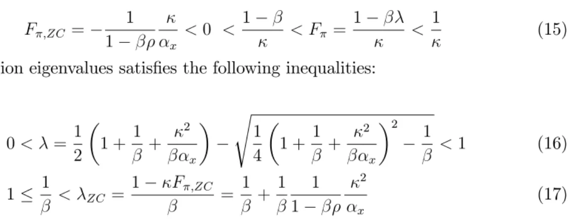
< 0 < 1 < F = 1 < 1 (15)

The in‡ation eigenvalues satis…es the following inequalities:

0 < = 1 2 1 + 1 + 2 x s 1 4 1 + 1 + 2 x 2 1 < 1 (16) 1 1 < ZC = 1 F ;ZC = 1 + 1 1 1 2 x (17) The policy instrument (or the Lagrange multiplier on forward-looking in‡ation) is optimally predetermined for Ramsey optimal policy whereas it is forward-looking with in…nite horizon zero-credibility policy. This implies an additional stable eigenvalue for Ramsey optimal policy with respect to zero-credibility policy, according to Blanchard and Kahn (1980) determinacy condition. QED.

Figures 1 and 2: In‡ation rule parameter and in‡ation eigenvalues functions of x for

Ramsey optimal policy (solid line) and zero-credibility policy (dash line) for = 0:995,

= 0:340; = 0:99. 2 4 6 8 10 -6 -4 -2 0 2 4

Cost of changing policy instrument Rule parameter 0 2 4 6 8 10 0 1 2 3

Cost of changing policy instrument Eigenvalue

The estimated parameters = 0:995, = 0:340for a given = 0:99of the Ramsey

op-timal policy model are found during Volcker-Greenspan’s Fed starting 1979q3-2006q2 in the next section. Figure 1 plots the positive-feedback in‡ation rule parameter F ;ZC < 0of

zero-credibility policy (dashed line) and respectively the negative-feedback in‡ation rule parameter F > 0 of Ramsey optimal policy (continuous line) as non-linear increasing (respectively decreasing) function of the relative cost of changing the policy instrument

x. The estimated parameters correspond to the point: x = 4:552 and F = 0:447.

Figure 2 plots the related eigenvalue ZC of zero-credibility policy (and respectively the

eigenvalue of Ramsey optimal policy) as non-linear decreasing (respectively

increas-ing) function of the relative cost of changing the policy instrument x. The estimated

parameters correspond to the point x = 4:552and = 0:856.

For an in…nite cost of changing the policy instrument ( x ! +1, the Fed has maximal

stable in‡ation eigenvalue tends to one for Ramsey optimal policy. For zero-credibility policy, the positive-feedback rule parameter F increases up to zero (with negative values).

The unstable in‡ation eigenvalue ZC decreases towards to 1= > 1.

For a near-zero cost of changing the policy instrument ( x ! 0, the Fed is an in‡ation

nutter), the negative-feedback rule parameter F increases to its largest bounded positive

value. The stable in‡ation eigenvalue tends to zero for Ramsey optimal policy. For

zero-credibility policy, the positive-feedback rule parameter decreases to minus in…nity

(with negative values). The unstable in‡ation eigenvalue ZC tends to plus plus in…nity.

3.2

Speci…cation tests of zero-credibility policy

Time-consistent policy is described by a permanent anchor of in‡ation on the output gap and by two AR(1) processes of in‡ation and of the output gap. Variables, such

as in‡ation ( t + ) are not computed as deviations of equilibrium (already denoted

t). Estimates of equilibrium values ( ; x ) are then sample mean values found in the

estimates of intercepts. The reduced form zero-credibility policy policy rule to be tested (which corresponds to a permanent anchor of in‡ation on the output gap) allows to estimate the reduced form zero-credibility policy rule parameter F ;ZC:

xt+ x = F ;ZC( t+ ) + (x F ;ZC ) + "x ;t with (18)

"x ;t = 0 for all dates, R2 = 1 and F ;ZC < 0

We assume i.i.d. measurement errors t for the in‡ation equation of Ramsey optimal

policy. By the same token, for the in…nite horizon zero-credibility policy, we also assume an i.i.d. measurement error "x ;t, for the policy rule equation, in order to avoid the

stochastic singularity of the perfect negative correlation predicted by the theory. A high R2 _{for the in‡ation equation would signal this measurement error to be su¢ ciently small}

and close to the theoretical model. For example, one can perform a one-sided test of a composite null hypothesis of a simple correlation very close to minus one: H0;ZC;SS :

rx < 0:99. A …rst speci…cation test of the negative sign restriction of zero-credibility

policy is more informative.

Negative sign restriction (NSR): H0;ZC;N S : rx < 0 (19)

A positive sign of the zero-credibility rule suggests Ramsey optimal policy as an alternative, with an opposite sign on the policy rule parameter F . The simple correlation between the output gap and in‡ation provides another estimate of the zero-credibility policy rule parameter F ;ZC = rx ";x= "; < 0. It is equal to the one found using the

ratio of standard errors of residuals of the AR(1) estimations for in‡ation and for the output gap : F ;ZC = ";x= "; only if the following condition is satis…ed: rx = 1

(stochastic singularity).

The rejection of stochastic singularity is expected to be stronger in the zero-credibility

policy rule with a lower R2 _{(because it does not include a lagged dependent variable)}

than the one of the Ramsey in‡ation equation (which includes lagged in‡ation). Hence, a second speci…cation test of zero-credibility policy versus Ramsey optimal policy is a Durbin (1970) test of the auto-correlation of residuals of these measurement errors of the zero-credibility positive-feedback policy rule. The measurement errors of the zero-zero-credibility policy rule should not be auto-correlated according to the theory of zero-credibility policy:

White noise disturbances: H0;ZC;Durbin: ";x = 0 for "x ;t = ";x "x ;t+ t with t i.i.d.

(20) If measurement errors are correlated, this alternative hypothesis suggests that at least one lagged policy instrument is missing in the regression of the policy rule. This is exactly a reduced form of the Ramsey optimal policy rule which also depends on in‡ation. Finally, we can perform another test. In the zero-credibility feedback rule, the policy instrument is a linear function of the policy target. The two AR(1) process for in‡ation and the output gap have common auto-correlation parameters:

t+ = ( t 1+ ) + (1 ) + NZC"u;t with "u;t i.i.d. (21)

xt+ x = (xt 1+ x ) + (1 ) x + F ;ZCNZC"u;t with "u;t i.i.d. (22)

We can test the hypothesis of a common auto-correlation parameter for the policy target (in‡ation) and for the policy instrument (output gap):

Common auto-correlation (CA): H0;ZC;CA : = x (23)

Proposition 2: For zero-credibility policy, only the auto-correlation coe¢ cient of the

cost-push shock can be identi…ed. But the four other structural parameters are not

identi…ed: the Fed’s preferences parameter x, the slope of the new-Keynesian Phillips

curve , the discount factor and the variance of the cost-push shock 2

";u. If the Fed’s

preferences is a welfare loss function, where Fed’s preferences parameter is endogenous ( x = _"), the representative household’s elasticity of substitution between each

di¤eren-tiated goods " is not identi…ed.

Proof. If common auto-correlation hypothesis is not rejected, the AR(1) estimates

of the policy target and of the policy instrument identify the auto-correlation parameter

of the non-observable cost-push shock: . The ratio of the standard errors of residuals

of each AR(1) estimations of in‡ation and output gap provides another estimate of the zero-credibility reduced form rule parameter F ;ZC, (if rx = 1), if the hypothesis of a

negative sign is not rejected:

F ;ZC = ";x= "; (24)

The variance 2

"; of perturbations of the in‡ation AR(1) process is: 2 "; = N 2 ZC 2 ";u) N 2 ZC = 2 "; 2 ";u (25) The cross equations covariance "; x between the residuals of both AR(1) process of

in‡ation and of the output gap does not allow to identify either the private sector reduced

form parameter NZC anchoring in‡ation on the cost-push shock or the variance of the

cost-push shock 2

";u. The simple correlation between the two residuals is predicted to be

exactly negatively correlated (r"; x = 1):

"; x = ";x "; 2 "; 2 ";u 2 ";u = ";x "; < 0: (26)

It is not possible to identify at least one of these four remaining structural parameters

four structural parameters:

F ;ZC =

1

1 x

< 0: (27)

Three identifying equations are missing in the case of zero-credibility policy. QED. Finally, the tests of reduced form parameters of bivariate VAR(1) of zero-credibility policy versus Ramsey optimal policy are not feasible. The exact multicollinearity (ex-act correlation) between regressors (current output gap and in‡ation) imply a bivariate

VAR(1) with in…nite coe¢ cients with denominator including the term 1 r2

x equal to zero: xt+1 t+1 = +1 1 1 +1 xt t + NZC F ;ZCNZC "t (28)

The zero-credibility policy equilibrium predicts that out-of-equilibrium behavior

cor-responds to a non-stationary bivariate VAR including one unstable eigenvalue ZC and

one stable eigenvalue , which cannot be estimated. By contrast, the stationary struc-tural VAR(1) of output gap and in‡ation with Ramsey optimal policy allows to identify a larger number of structural parameters.

xt+1 t+1 = a b c d xt t + Fu;R 0 "t

Two additional reduced form parameters (b; c) are available, because the stable sub-space of the VAR process is of dimension two with Ramsey optimal policy instead of dimension one with zero-credibility policy.

4

Tests with Output Gap as Policy Instrument

4.1

Speci…cation tests

The annualized quarter-on-quarter rate of in‡ation and the congressional budget o¢ ce (CBO) measure of the output gap are taken from Mavroeidis’ (2010) online appendix (detailed information at the end of this paper’s appendix). The pre-Volcker sample covers the period 1960q1 to 1979q2 and the Volcker-Greenspan sample runs until 2006q2. The period of Paul Volcker’s tenure is 1979q3 to 1987q2. The period of Alan Greenspan’s tenure is 1987q3 to 2006q1.

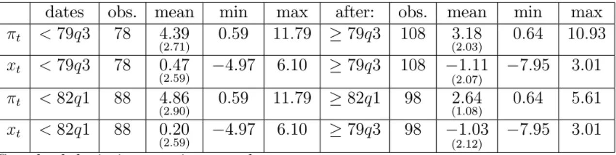
According to Debortoli and Nunes (2015), a structural break corresponds to an new initial anchor of forward in‡ation on the output gap for Ramsey optimal policy with …nite horizon. Clarida, Gali and Gertler (2000) and Mavroeidis (2010) consider the beginning of Paul Volcker’s mandate 1979q3 as a structural break. Givens (2012) considers 1982q1 as a structural break, after 1981 fall of in‡ation and before the 1982 recession. Matthes (2015) estimation of the private sectors beliefs regarding central bank regimes also points to 1982q1 as a structural break. Table 2 presents summary statistics before and after the 1979q3 and 1982q1 structural breaks.

dates obs. mean min max after: obs. mean min max t < 79q3 78 4:39 (2:71) 0:59 11:79 79q3 108 3:18 (2:03) 0:64 10:93 xt < 79q3 78 0:47 (2:59) 4:97 6:10 79q3 108 (2:07)1:11 7:95 3:01 t < 82q1 88 4:86 (2:90) 0:59 11:79 82q1 98 (1:08)2:64 0:64 5:61 xt < 82q1 88 0:20 (2:59) 4:97 6:10 79q3 98 1:03 (2:12) 7:95 3:01

Standard deviations are in parentheses.

The mean of in‡ation and of output gap are lower during Volcker-Greenspan than before Volcker. Excluding the period 1979q3 to 1981q4, in particular the sharp disin‡ation which occurred during 1981 (…gure 3), the standard error of in‡ation decreases by half from 2.03 to 1.08 .

Table 3: Pre-tests of zero-credibility policy rule

Dates obs rx Low 95% r p R2x F ;ZC c ";x

< 79q3 78 0:13 0:21 < 0:001 0:02 0:13 (0:11) 1:03 (0:56) 0:92 (0:04) < 82q1 108 0:30 0:42 < 0:001 0:09 0:30 (0:09) 0:14 (0:35) 0:91 (0:04) 79q3 88 0:24 0:31 < 0:001 0:06 0:22 (0:09) 1:25 (0:53) 0:92 (0:05) 82q1 98 0:40 0:53 < 0:001 0:16 0:78 (0:18) 1:03 (0:52) 0:89 (0:05)

The pre-tests of the null hypothesis of a quasi perfect negative correlation H0 : rx <

0:99 between observed in‡ation and observed output gap are rejected. The test uses

Fisher’s Z transformation using the procedure corr with the software SAS. The threshold

of the composite null hypothesis 0:99 is far away from the 95% single tail con…dence

interval, where the lowest 95% con…dence limit reported in table 3 is at most equal to

0:53 for the period beginning from 1982q1 (…gure 4). The opposite null hypothesis

H0 : r (xt; t) = 0 is not rejected before 1979q3. zero-credibility policy predicts a perfect

correlation for the anchor of in‡ation expectations with the output gap. If the zero-credibility policy equilibrium occurred before 1979q3, we do not reject the null hypothesis H0 : r (Et 1( t) ; t) = 0 that the rational expectations of in‡ation are orthogonal to

observed in‡ation.

The pre-tests of the null hypothesis of the auto-correlation of residuals H0 : ";x = 0

are strongly rejected, with a point estimate at least equal to 0:89 (…gure 5). These tests gives a hint of model misspeci…cation. They suggest an omitted lagged policy instrument in the policy rule. When it is included in Ramsey optimal policy rule, the R2 _increases

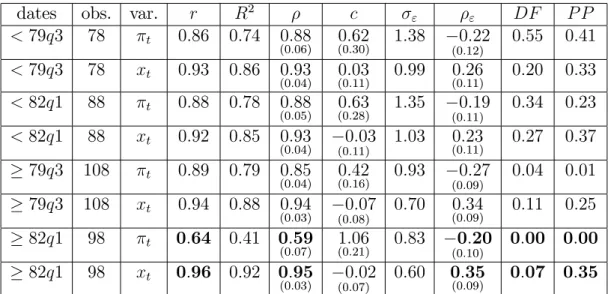
from 16% (table 3, last line) to 93% (table 6, last line) beginning in 1982q1. Table 4: Auto-correlation of in‡ation and output gap

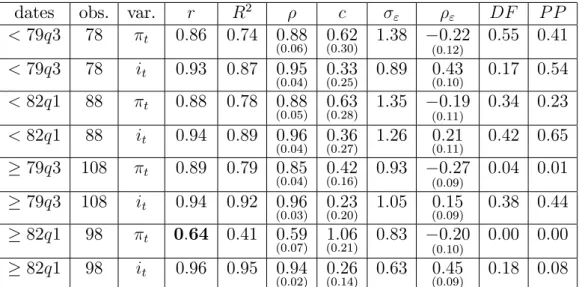
dates obs. var. r R2 _c " " DF P P < 79q3 78 t 0:86 0:74 0:88 (0:06) 0:62 (0:30) 1:38 0:22 (0:12) 0:55 0:41 < 79q3 78 xt 0:93 0:86 0:93 (0:04) 0:03 (0:11) 0:99 0:26 (0:11) 0:20 0:33 < 82q1 88 t 0:88 0:78 0:88 (0:05) 0:63(0:28) 1:35 (0:11)0:19 0:34 0:23 < 82q1 88 xt 0:92 0:85 0:93 (0:04) (0:11)0:03 1:03 0:23 (0:11) 0:27 0:37 79q3 108 t 0:89 0:79 0:85 (0:04) 0:42(0:16) 0:93 (0:09)0:27 0:04 0:01 79q3 108 xt 0:94 0:88 0:94 (0:03) (0:08)0:07 0:70 0:34 (0:09) 0:11 0:25 82q1 98 t 0:64 0:41 0:59 (0:07) 1:06(0:21) 0:83 (0:10)0:20 0:00 0:00 82q1 98 xt 0:96 0:92 0:95 (0:03) (0:07)0:02 0:60 0:35 (0:09) 0:07 0:35

Table 4 investigates the auto-correlation and unit roots of in‡ation and output gap. The output gap and in‡ation are highly auto-correlated (respectively 0.93 and 0.86), except when in‡ation excludes the 1981 disin‡ation for the period after 1981q4. For the period 1982q1 to 2006q2, the in‡ation auto-correlation coe¢ cient falls in the 95%

con…dence interval 0:6 0:14 and it is statistically di¤erent from the output gap

auto-correlation coe¢ cient in the 95% con…dence interval 0:95 0:06 (…gures 4 and 5). As

the zero-credibility policy equilibrium predicts that the auto-correlation of the output gap and of in‡ation should be the same, this is an additional test against zero-credibility policy, which holds for the period 1982q1 to 2006q2.

There is a negative auto-correlation of residuals " for in‡ation and a (statistically

signi…cant at the 5% level) positive auto-correlation of residuals for the output gap. The column DF reports the p-value of the Dickey-Fuller test of unit root with one lag without trend. The column PP reports the p-value of the Phillips-Perron test of unit root, which takes into account auto-correlation, with one lag without trend. The null hypothesis of a unit root is rejected for in‡ation after 1979q2 and after 1981q4.

4.2

Tests of Ramsey Optimal Policy

Table 5 presents estimates of structural parameters, Table 5 report estimates of three

structural VAR estimations for ( ; R; F ;R), ; R; x and ( ; ( ) ; x( )) with two

given values for the discount factor = 1 or = 0:99for the Volcker-Greenspan period.

With these three estimations, delta method is not necessary to compute the standard errors of parameters in each case. Maximum likelihood did not converge for pre-Volcker period (unconstrained VAR corresponds to complex conjugate eigenvalues, which are excluded because of exogenous real auto-correlation of cost-push shock). Post 1982q1 estimations converged to unlikely estimates.

Table 5: Ramsey optimal policy structural parameters

Dates F x ₌ 1 " ( ) x( ) Fu;R( ) u( ) 79q3 0:995 (0:024) 0:857(0:054) 0:447(0:292) 13:375(6:627) 1 0:321(0:303) 4:296(5:447) 3:027 0:229 79q3 0:995 (0:024) 0:857(0:054) 0:447(0:292) 13:375(6:627) 0:99 0:340(0:314) 4:552(5:703) 2:861 0:242

The cost-push shock faces is extremely persistent, close to a unit root, with estimate close to one. The ratio x _{is statistically signi…cant. If the Fed’s preferences are identical}

to (welfare) household’s preferences), then x ₌ 1

" and " = 0:07. The new-Keynesianb

relatively large (although not unheard of in previous estimations). for the period 1979-2006.

Table 6: In‡ation and output gap structural (S) versus unconstrained (U) VAR

dates obs. var. S/U t 1 xt 1 c " R2

79q3 108 t S 0:85 0:009 0:428 (0:16) (0:09)0:25 0:793 0:857 (0:054) 79q3 108 t U 0:85 (0:04) 0:009(0:04) (0:16)0:43 (0:09)0:25 0:79 0:85 79q3 108 xt S 0:064 0:999 0:198 (0:121) 0:29(0:09) 0:888 0:995(0:024) 79q3 108 xt U 0:084 (0:03) 0:917 (0:03) 0:17 (0:11) 0:29 (0:09) 0:89 0:92

Table 6 compares the reduced form parameters of the VAR of Ramsey optimal policy with parameters of an unconstrained VAR. The in‡ation equation of the VAR are the same up to the third decimal of all statistics. For the output gap equation, Ramsey optimal policy slightly over-estimates the persistence of the output gap: its VAR auto-correlation parameter shifts from 0:93 to 1. For the output gap rule, the auto-auto-correlation of residuals fell from 0:92 with zero-credibility policy to 0:29 with Ramsey optimal policy, but it remains statistically signi…cant. As well, the in‡ation equation has a statistically signi…cant auto-correlation ( 0:25).

The reduced form Ramsey optimal policy rule of the structural VAR is observationally equivalent to the LQR …rst step representation including the non-observable cost-push shock, when taking into account the other equations of the Hamiltonian system:

Ramsey : xt = 0:995xt 1 0:064 t 1 2:861"u;t or xt= 0:447 t 2:861ut for = 0:99

(29) The policy instrument responds to two variables for Ramsey stable subspace of dimen-sion two. The policy instrument responds to one variable in the zero-credibility policy stable subspace of dimension one. The reduced form policy rule for zero-credibility policy is:

Time-consistent: xt= 0:22 t (30)

5

Tests with Federal Funds Rate Smoothing and

Work-ing Capital Channel

5.1

Speci…cation tests

Assuming the polar case where all labor cost is …nanced by working capital instead than no labor cost at all, the federal funds rate is used here as a policy instrument. Its variance enters into the period loss function t2+ ii2t as an interest smoothing model. Figure 2

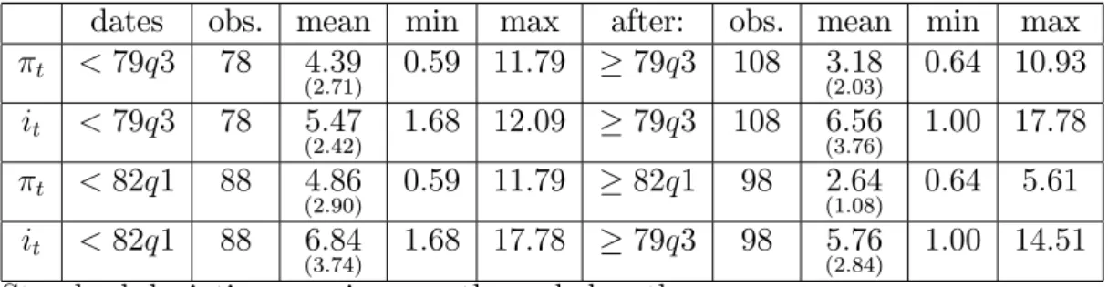
represents the time series of in‡ation and federal funds rate. Table 2 presents summary statistics before and after the 1979q3 and 1982q1 structural breaks.

dates obs. mean min max after: obs. mean min max t < 79q3 78 4:39 (2:71) 0:59 11:79 79q3 108 3:18 (2:03) 0:64 10:93 it < 79q3 78 5:47 (2:42) 1:68 12:09 79q3 108 (3:76)6:56 1:00 17:78 t < 82q1 88 4:86 (2:90) 0:59 11:79 82q1 98 2:64 (1:08) 0:64 5:61 it < 82q1 88 6:84 (3:74) 1:68 17:78 79q3 98 (2:84)5:76 1:00 14:51

Standard deviations are in parentheses below the mean.

The means of in‡ation are lower after Volcker than before Volcker. Excluding the period 1979q3 to 1981q4, in particular the sharp disin‡ation which occurred during 1981 (…gure 3), the standard error of in‡ation decreases by half from 2.03 to 1.08. The di¤er-ence of means between the policy interest rate and in‡ation increased after Volcker.

Table 3B: Pre-test of zero-credibility policy rule

dates obs ri t ri = 0 : p R2i F ;D c ";i

< 79q3 78 0:83 12:85 < 0:001 0:68 0:74 (2:22) 2:22 (0:30) 0:61 (0:09) < 82q1 88 0:79 11:83 < 0:001 0:62 1:01 (0:08) (0:48)1:55 0:73(0:08) 79q3 108 0:75 11:63 < 0:001 0:56 1:39 (0:12) 1:39 (0:11) 0:76 (0:06) 82q1 98 0:53 6:08 < 0:001 0:28 1:39 (0:22) (0:65)2:09 0:80(0:06)

The tests of the null hypothesis of a quasi perfect negative correlation H0 : ri < 0:99

between in‡ation and federal funds rate have been replaced by the usual tests of the null hypothesis: H0 : ri = 0, because ri > 0. The negative sign of the zero-credibility policy

rule is rejected, with large t statistics. The Durbin and Breusch-Godfrey tests strongly reject the lack of serial correlation (for one or two lags) with p-value below 10 4_{. Tests}

of the null hypothesis of the …rst order auto-correlation of residuals H0 : ";i = 0 are

rejected, with a point estimate at least equal to 0:60 and at most 0:80. The in…nite horizon zero-credibility positive-feedback mechanism does not …t the data when the cost of capital is taken into account into the monetary transmission mechanism. Finally, the Taylor principle (an in‡ation coe¢ cient F larger than one) is not satis…ed before Volcker and satis…ed after Volcker.

Table 4B investigates the auto-correlation of in‡ation and federal funds rate. In‡ation and Federal funds rate are highly auto-correlated (respectively 0.93 and 0.86), except for the period 1982q1 to 2006q2, the in‡ation auto-correlation coe¢ cient falls in the 95% con…dence interval 0:6 0:14 and it is statistically di¤erent from the federal funds rate

auto-correlation coe¢ cient in the 95% con…dence interval 0:95 0:02. In…nite horizon

zero-credibility policy predict that the auto-correlation should be the same, which is not the case after 1982q1.

dates obs. var. r R2 _c " " DF P P < 79q3 78 t 0:86 0:74 0:88 (0:06) 0:62 (0:30) 1:38 0:22 (0:12) 0:55 0:41 < 79q3 78 it 0:93 0:87 0:95 (0:04) 0:33 (0:25) 0:89 0:43 (0:10) 0:17 0:54 < 82q1 88 t 0:88 0:78 0:88 (0:05) 0:63(0:28) 1:35 (0:11)0:19 0:34 0:23 < 82q1 88 it 0:94 0:89 0:96 (0:04) 0:36(0:27) 1:26 (0:11)0:21 0:42 0:65 79q3 108 t 0:89 0:79 0:85 (0:04) 0:42 (0:16) 0:93 0:27 (0:09) 0:04 0:01 79q3 108 it 0:94 0:92 0:96 (0:03) 0:23 (0:20) 1:05 0:15 (0:09) 0:38 0:44 82q1 98 t 0:64 0:41 0:59 (0:07) 1:06(0:21) 0:83 (0:10)0:20 0:00 0:00 82q1 98 it 0:96 0:95 0:94 (0:02) 0:26(0:14) 0:63 (0:09)0:45 0:18 0:08

There is a negative auto-correlation of residuals " for in‡ation and a positive

auto-correlation of residuals for federal funds rate. The column DF reports the p-value of the Dickey-Fuller test of unit root with one lag without trend. The column PP reports the p-value of the Phillips-Perron test of unit root, which takes into account auto-correlation, with one lag without trend. The null hypothesis of a unit root is rejected at the 5% threshold for in‡ation after 1979q2 and after 1981q4. It is rejected for federal funds rate at the 10% level after 1981q4 only for the Phillips-Perron test.

5.2

Tests of Ramsey optimal policy

Table 5B reports estimates using four structural VAR estimations for ( ; C; F ;C), for

; C; i

i and for ( ; ( ) ; i( )) with the identi…cation restrictions for the credibility adjusted discount factor. We check that these three estimations are observationally equiv-alent. In particular, each estimate satisfy the theoretical relations with the others implied by Ramsey optimal policy. When the federal funds rate is the policy instrument, the es-timations only converged to plausible values for the pre-Volcker period, before 1979q3.

The implicit rule parameter on the cost-push shock is computed using Fu( ) = ₁ 1 F

and the variance of the cost push shock is u( ) = _F";i_{u( )} with the root mean square

error of the residuals of the policy instrument equation equal to ";i = 0:876.

Table 5B: Ramsey optimal policy structural parameters

Dates F i i( ) i( ) Fu;C( ) u( ) < 79q3 0:550 (0:092) 0:947(0:047) 0:873(0:131) 20:83(18:26) 1 0:060(0:06) 1:24(0:34) 1: 822 0:481 < 79q3 0:550 (0:092) - - - 0:99 0:071(0:06) 1:47(0:36) 1: 802 0:486 < 79q3 0:550 (0:092) - - - 0:94 0:125(0:063) 2:60(0:16) 1: 710 0:512 < 79q3 0:550 (0:092) - - - 0:93 0:136(0:064) 2:83(1:35) 1: 693 0:517 < 79q3 0:550 (0:092) - - - 0:92 0:146(0:065) 3:05(1:54) 1: 676 0:522

Estimates of structural parameters are plausible values. The Fed’s reduced form rule parameter F is signi…cantly di¤erent from zero at the 5%. To reach the

statisti-cal signi…cance at the 5% level of both i( ) and i( ) and not only one of the two

parameters is obtained for identi…cation restrictions of the credibility adjusted discount

factor _{2 [0:92; 0:94]. This corresponds to a Fed’s probability to commit in this range:}

only the Fed’s preference i( ) is statistically signi…cant. For < 0:92, only the slope

of the new-Keynesian Phillips curve for working capital i( )is statistically signi…cant.

When the identi…cation restriction on increases, both estimates i( ) and i( )

in-crease, but not at the same pace.

Table 6B shows that the reduced form parameters of the structural VAR(1) (rows S) are identical to the unconstrained VAR(1) estimates (rows U) up to the third decimal.

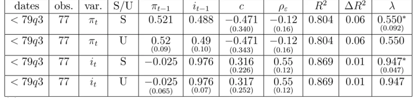
Table 6B: In‡ation and federal funds rate structural (S) versus uncon-strained (U) VAR

dates obs. var. S/U t 1 it 1 c " R2 R2

< 79q3 77 t S 0:521 0:488 0:471 (0:340) 0:12 (0:16) 0:804 0:06 0:550 (0:092) < 79q3 77 t U 0:52 (0:09) 0:49(0:10) (0:343)0:471 0:12 (0:16) 0:804 0:06 0:550 < 79q3 77 it S 0:025 0:976 0:316 (0:226) (0:12)0:55 0:869 0:01 0:947(0:047) < 79q3 77 it U 0:025 (0:065) 0:976 (0:07) 0:317 (0:252) 0:55 (0:12) 0:869 0:01 0:947

(1) For the in‡ation equation, there is Granger causality from lagged federal funds rate to in‡ation. The exogenous cost-push shock correlation is close to the auto-correlation of in‡ation in the VAR. The residuals are not auto-correlated controlling for endogenous lagged in‡ation and federal funds according to Durbin’s test. The autocorre-lation estimate is 0:12, It not statistically di¤erent from zero (Durbin’s test: t = 0:77, p = 0:44).

(2) For the federal funds rate rule equation, the auto-correlation 0:976 is relatively close to a unit root. The endogenous stable eigenvalue corresponds to the auto-correlation of the federal funds rate.

One can compare our modest results with two recent papers using implicit functions of the parameters within a reduced form VAR including three US time-series (in‡ation, output gap and Federal funds rate). Givens (2012) …nds out that Volcker-Greenspan pe-riod corresponds to zero-credibility policy whereas Matthes (2015) …nds it corresponds to Ramsey optimal policy. The ratio of the estimated weight on output in the loss function

in commitment versus discretion in Givens (2012): bD=bC = 0:0987=0:1351 = 0:7 and

10 times larger in Matthes (2015) bD=bC = 0:49=0:07 = 7. For the transmission

mech-anism, Givens (2012) estimate of the intertemporal elasticity of substitution is 0:0089 (estimated standard error 0:0035, 95% con…dence interval [0:0019; 0:0159]) for Ramsey optimal policy and 0:0002 for zero-credibility policy, with an estimated standard error

0:0001so that zero belong to the 95% con…dence interval. Matthes (2015) estimate is 70

times larger 1=1:61 = 0:62 for both policies. The estimated standard error of this para-meter is not disclosed. Givens (2012) estimate of the slope of the new-Keynesian Phillips

curve is _{b = 0:0045, with estimated standard error 0:0016 and 95% con…dence}

inter-val [0:0019; 0:0159]), for Ramsey optimal policy and 0:0047 for discretion with estimated standard error 0:009 so that zero belongs to the 95% con…dence interval ("Estimates of are small but within the range typical of the literature." p.1043). In the discretion regime, both transmission mechanism parameters for the Federal funds rate not statistically dif-ferent from zero. This result supports the hypothesis of monetary policy ine¤ectiveness

during 1982-2006. Matthes (2015) estimate is 75 times larger: _{b = 0:7=(1 + 0:99) =}

0:35: "The estimate found here, while being at the other end, is not unheard of ". The estimated standard error of this parameter is not disclosed.

Givens (2012) assumes one lag of in‡ation, two lags of output and one lag for Federal funds rate. Matthes (2015) assumes one lag of in‡ation and two exogenous auto-regressive

forcing variables. The more lags of observable exogenous variables are added in the speci…cation of the new-Keynesian Phillips curve, the more likely the weak identi…cation of some parameters occurs (Mavroeidis (2005), Mavroeidis et al. (2014), Dees, Pesaran, Smith, Smith (2009), Canova and Sala (2009), Komunjer and Ng (2012) and Iskrev (2012)).

6

Conclusion

Using closed form solutions of Ramsey optimal policy and zero-credibility policy, we take exactly into account the identi…cation restrictions related to the dimension of the stable subspace of each policy. Ramsey optimal policy with quasi-commitment has a comparative advantage with respect to in…nite horizon zero-credibility policy for mod-elling persistence with fewer parameters. Further work may extend this approach to other transmission mechanisms than the new-Keynesian Phillips curve with labor cost channel or with working capital channel.

References

[1] Adjemian S. and Devulder A. (2011). Evaluation de la politique monétaire dans un modèle DSGE pour la zone euro. Revue française d’économie, 26(1), 201-245. [2] Adolfson, M., Laséen, S., Lindé, J., & Svensson, L. E. (2011). Optimal Monetary

Policy in an Operational Medium-Sized DSGE Model. Journal of Money, Credit and Banking, 43(7), 1287-1331.

[3] Anderson E.W., Hansen L.P., McGrattan E.R. and Sargent T.J. (1996). Mechanics of Forming and Estimating Dynamic Linear Economies. in Amman H.M., Kendrick D.A. and Rust J. (editors) Handbook of Computational Economics, Elsevier, Ams-terdam, 171-252.

[4] Backus, D., & Dri¢ ll, J. (1986). The consistency of optimal policy in stochastic rational expectations models (No. 124). CEPR Discussion Papers.

[5] Blanchard O.J. and Kahn C. (1980). The solution of linear di¤erence models under rational expectations. Econometrica, 48, pp. 1305-1311.

[6] Blinder A.S. (1986). More on the speed of adjustment in inventory models. Journal of Money, Credit and Banking, 18, 355–365.

[7] Bratsiotis, G. J. and Robinson, W. A. (2016). Unit Total Costs: An Alternative Marginal Cost Proxy for In‡ation Dynamics. Macroeconomic Dynamics, 1-24. [8] Canova, F., & Sala, L. (2009). Back to square one: Identi…cation issues in DSGE

models. Journal of Monetary Economics, 56(4), 431-449.

[9] Castelnuovo E. and Surico P. (2004). Model uncertainty, optimal monetary policy and the preferences of the Fed. Scottish Journal of Political Economy, 51(1), pp. 105-126.

[10] Castelnuovo E. (2006). The Fed’s preferences for Policy Rate Smoothing: Overes-timation due to misspeci…cation? The B.E. Journal in Macroeconomics (Topics), 6(2), article 5.

[11] Cecchetti S. and Ehrmann M. (2002), “Does In‡ation Targeting Increase Output

Volatility? An International Comparison of Policymakers Preferences and

Out-comes,” in Loayza, Norman, and Klaus Schmidt-Hebbel (eds.), Monetary Policy: Rules and Transmission Mechanisms, vol. 4 of Series on Central Banking, Analysis, and Economic Policies, Central Bank of Chile, 247— 274.

[12] Chatelain, J. B., and Ralf, K. (2017a). Publish and Perish: Creative Destruction and Macroeconomic Theory. Available at SSRN: https://ssrn.com/abstract=2915860.

[13] Chatelain, J. B., and Ralf, K. (2017b). Hopf bifurcation from

new-Keynesian Taylor rule to Ramsey optimal policy (2017). Available at SSRN: https://papers.ssrn.com/sol3/papers.cfm?abstract_id=2971227.

[14] Chatelain, J. B., and Ralf, K. (2017c). A Simple Algorithm for Solving Ramsey Optimal Policy with Exogenous Forcing Variables. Econstor working paper.

[15] Chari, V. V., & Kehoe, P. J. (1990). Sustainable plans. Journal of political economy, 98(4), 783-802.

[16] Christiano, L. J., Trabandt T. and Walentin K. (2011). DSGE models for mone-tary policy analysis in Handbook of monemone-tary economics, editors BM Friedman, M. Woodford, volume 3A.

[17] Clarida R., Gali J. and Gertler M. (1999). The Science of Monetary Policy: a new Keynesian Perspective. Journal of Economic Literature, 37(4), 1661-1707.

[18] Clarida R., Gali J. and Gertler M. (2000). Monetary Policy Rules and Macro-economic Stability: Evidence and Some Theory. Quarterly Journal of Economics, 115(1), pp. 147-180.

[19] Cochrane J.H. (2011). Determinacy and Identi…cation with Taylor Rules. Journal of Political Economy, 119(3), pp. 565-615.

[20] Cohen D. and Michel P. (1988). How Should Control Theory Be Used to Calculate a Time-Consistent Government Policy? Review of Economic Studies, 55, 119(3), 263-274.

[21] Debortoli, D., and Nunes, R. (2014). Monetary regime switches and central bank preferences. Journal of Money, Credit and Banking, 46(8), 1591-1626.

[22] Debortoli, D., & Lakdawala, A. (2016). How credible is the Federal Reserve? A struc-tural estimation of policy re-optimizations. American Economic Journal: Macroeco-nomics, 8(3), 42-76.

[23] Dees, S., Pesaran, M. H., Smith, L. V., & Smith, R. P. (2009). Identi…cation of new Keynesian Phillips curves from a global perspective. Journal of Money, Credit and Banking, 41(7), 1481-1502.

[24] Duarte, P. G. (2009). A feasible and objective concept of optimal monetary policy: The quadratic loss function in the postwar period. History of Political Economy, 41(1), 1-55.

[25] Durbin, J. (1970). Testing for serial correlation in least-squares regressions when some of the regressors are lagged dependent variables. Econometrica 38: 410–421. [26] Favero, C. A., & Rovelli, R. (2003). Macroeconomic stability and the preferences of

the Fed: A formal analysis, 1961-98. Journal of Money, Credit, and Banking, 35(4), 545-556.

[27] Fève P., Matheron J. and Poilly C. (2007). Monetary Policy Dynamics in the Euro Area. Economics Letters, 96(1), 97-102.

[28] Fujiwara, I., Kam, T., & Sunakawa, T. (2016). A note on imperfect credibility. SSRN working paper.

[29] Gali J. (2015). Monetary Policy, In‡ation, and the Business Cycle, (2nd edition) Princeton University Press.

[30] Giannoni, M., & Woodford, M. (2004). Optimal in‡ation-targeting rules. In The In‡ation-Targeting Debate (pp. 93-172). NBER, University of Chicago Press. [31] Giordani and Söderlind (2004). Solution of Macromodels with Hansen-Sargent

Ro-bust Policies: some extensions. Journal of Economic Dynamics and Control, 12, 2367-2397.

[32] Givens, G. E. (2012). Estimating central bank preferences under commitment and discretion. Journal of Money, credit and Banking, 44(6), 1033-1061.

[33] Griliches, Z. (1967). Distributed lags: a survey. Econometrica 35, 16–49.

[34] Hansen L.P. and Sargent T. (2008). Robustness, Princeton University Press, Prince-ton.

[35] Havranek, T., Rusnak, M., & Sokolova, A. (2017). Habit formation in consumption: A meta-analysis. European Economic Review, 95, 142-167.

[36] Ilbas, P. (2012). Revealing the preferences of the US Federal Reserve. Journal of Applied Econometrics, 27(3), 440-473.

[37] Iskrev, N. (2010). Local identi…cation in DSGE models. Journal of Monetary Eco-nomics, 57(2), 189-202.

[38] Juillard M., Karam P.D., Laxton D., Pesenti P.A. (2006). Welfare-based monetary policy rules in an estimated DSGE model of the US. ECB working paper 613. [39] Kara, H. (2007). Monetary policy under imperfect commitment: Reconciling theory

with evidence. International Journal of Central Banking. 3(1), 149-177.

[40] Kollmann R. (2002). Monetary policy rules in the open economy: e¤ects on welfare and business cycles. Journal of Monetary Economics, 49(5), 989-1015.

[41] Kollmann, R. (2008). Welfare-maximizing operational monetary and tax policy rules. Macroeconomic dynamics, 12(S1), 112-125.

[42] Komunjer, I., & Ng, S. (2011). Dynamic identi…cation of dynamic stochastic general equilibrium models. Econometrica, 79(6), 1995-2032.

[43] Kydland F. and Prescott E.C. (1980). Dynamic Optimal Taxation, Rational Ex-pectations and Optimal Control. Journal of Economic Dynamics and Control, 2, pp.79-91.

[44] Leeper, E. M. (1991). Equilibria under ‘active’ and ‘passive’ monetary and …scal policies. Journal of monetary Economics, 27(1), 129-147.

[45] Levieuge G., Lucotte Y. (2014). A Simple Empirical Measure of Central Banks’ Conservatism, Southern Economic Journal, 81(2). 409-434.

[46] Ljungqvist L. and Sargent T.J. (2012). Recursive Macroeconomic Theory. 3rd edition. The MIT Press. Cambridge, Massaschussets.

[47] Matthes, C. (2015). Figuring Out the Fed— Beliefs about Policymakers and Gains from Transparency. Journal of Money, credit and Banking, 47(1), 1-29.

[48] Mavroeidis, S. (2005). Identi…cation issues in forward-looking models estimated by GMM, with an application to the Phillips curve. Journal of Money, Credit, and Banking, 37(3), 421-448.

[49] Mavroeidis S. (2010). Monetary Policy Rules and Macroeconomic Stability: some new Evidence. American Economic Review. 100(1), pp. 491-503.

[50] Mavroeidis S., Plagbord-Moller M., Stock J.M. (2014). Empirical Evidence on In-‡ation Expectations in the New Keynesian Phillips Curve. Journal of Economic Literature. 52(1), pp.124-188.

[51] McManus, D.A., Nankervis, J.C., Savin, N.E. (1994). Multiple optima and asymp-totic approximations in the partial adjustment model. Journal of Econometrics 62, 91–128.

[52] Oudiz G. and Sachs J. (1985). International Policy Coordination in Dynamic Macro-economic Models, in W.H. Buiter and R.C. Marston (eds), International Economic Policy Coordination, Cambrdige, Cambridge University Press.

[53] Ozlale, U. (2003). Price stability vs. output stability: tales of federal reserve admin-istrations, Journal of Economic Dynamics and Control, 27(9), 1595-1610.

[54] Paez-Farrell J. (2015). Taylor rules, central bank preferences and in‡ation targeting. Working Paper, university of She¢ eld.

[55] Quah, D., & Vahey, S. P. (1995). Measuring core in‡ation. The Economic Journal, 1130-1144.

[56] Roberds, W. (1987). Models of policy under stochastic replanning. International Economic Review, 731-755.

[57] Salemi, M. K. (1995). Revealed preference of the Federal Reserve: using inverse-control theory to interpret the policy equation of a vector autoregression. Journal of Business & Economic Statistics, 13(4), 419-433.

[58] Salemi, M. K. (2006). Econometric policy evaluation and inverse control. Journal of Money, Credit, and Banking, 38(7), 1737-1764.

[59] Salemi, M. K. (2010). It’s what they do, not what they say. The New International Monetary System: Essays in Honour of Alexander Swoboda, chapter 11, p;162. [60] Schaumburg, E., and Tambalotti, A. (2007). An investigation of the gains from

commitment in monetary policy. Journal of Monetary Economics, 54(2), 302-324. [61] Sims C.A. (1980). Macroeconomics and Reality. Econometrica, 48, 1-48.

[62] Simon H.A. (1956). Dynamic Programming under Uncertainty with a Quadratic Criterion Function. Econometrica, 24(1), 74-81.

[63] Söderlind P. (1999). Solution and estimation of RE macromodels with optimal policy. European Economic Review, 43(4), 813-823.

[64] Söderström, U., Söderlind, P., & Vredin, A. (2005). New-Keynesian Models and Monetary Policy: A Re-examination of the Stylized Facts. The Scandinavian journal of economics, 107(3), 521-546.

7

Appendix 1: De…nition of data variables

Mavroeidis data are running from 1960-Q1 to 2006-Q2.

In‡ation is annualized quarter-on-quarter rate of in‡ation, 400 * LN( GDPDEF/ GDPDEF(-1)) with GDPDEF: Gross Domestic Product Implicit Price De‡ator, 2000=100, Seasonally Adjusted. Released in August 2006. Source: U.S. Department of Commerce, Bureau of Economic Analysis.

GAPCBO is the output gap measure: 100 * LN(GDPC1/GDPPOT) with GDPC1: Real Gross Domestic Product, Billions of Chained 2000 Dollars, Seasonally Adjusted Annual Rate, Released in August 2006. Source: U.S. Department of Commerce, Bureau of Economic Analysis and GDPPOT: Real Potential Gross Domestic Product, Billions of Chained 2000 Dollars. Source: U.S. Congress, Congressional Budget O¢ ce.

Federal Funds Rate : Averages of Daily Figures - Percent, Source: Board of Governors of the Federal Reserve System

7.1

Appendix 2: Augmented Discounted Linear Quadratic

Reg-ulator

The new-Keynesian Phillips curve can be written as a function of the Lagrange multiplier where > 0, 0 < < 1 and 0 < q < 1 (Debortoli and Nunes (2014, appendix A). We

keep Gali (2015) chapter 5 t+1 notation of the Lagrange multiplier with one step ahead

subscript: it corresponds to Debortoli and Nunes (2014) notation t. Our notation for

the stable eigenvalue corresponds to Debortoli and Nunes (2014) notations " y = 1= ".

Et t+1+ 2 q x t+1= 1 q t 1 qut 1 q q Et j t+1

In what follows, refers to q to simplify notations. The solution of the Hamiltonian system are based on the demonstrations of the augmented discounted linear quadratic regulator in Anderson, Hansen, McGrattan and Sargent [1996], following the steps in Chatelain and Ralf (2017c):

0 @ 1 2 x 0 0 1 0 0 0 1 1 A 0 @ t+1t+1 ut+1 1 A = 0 @ 1 ₀ 1 1 1 0 0 0 1 A 0 @ tt ut 1 A + 0 @ 1 q q Et j t+1 0 0 1 A The Hamiltonian system is:

0 @ t+1t+1 ut+1 1 A = 0 @ 1 ₊ 2 x 2 x 1 1 1 0 0 0 1 A 0 @ tt ut 1 A + 0 @ 1 q q Et j t+1 0 0 1 A The characteristic polynomial of this upper square matrix is:

2 _{1 +} 1 ₊ 2

x

+ 1 = 0

The Hamiltonian matrix has two stable roots and ( is denoted in Gali (2015))

and one unstable root 1 . The determinant of the matrix is 1 = 1. Then <q1 <

1 _{. The trace of the matrix is}

= 1 2 0 @1 + 1 + 2 x s 1 + 1 + 2 x 2 4 1 A Identi…cation of

x: The characteristic polynomial is equal to zero. The policy rule parameter with respect to in‡ation depends on

x: (1 ) 1 1 = 2 x =₎ 1 1 = x =₎ F = 1 = 1 x

Hamiltonian system function of the stable eigenvalue (eliminating

x): 0 @ t+1t+1 ut+1 1 A = 0 @ + 1 1 1 + 1 1 1 1 1 0 0 0 1 A 0 @ t+1t+1 ut+1 1 A

Proposition 1: Solution of Ricatti and Sylvester equation: Rule parameters

t = P t+ Puut+ Pzzt (31) P = 1 1 , Pu = 1 1 1 1 = 1 1 1and Pz = 1 1 1 1 = 1 1 1 (32)

Demonstration: It uses the method of undetermined coe¢ cients of Anderson, Hansen,

McGrattan and Sargent’s (1996), section 5. The solution is the one that stabilizes the state-costate vector for any initialization of in‡ation 0 and of the exogenous variables

u0 in a stable subspace of dimension two within a space of dimension three ( t; t; ut) of

the Hamiltonian system. We seek a characterization of the Lagrange multiplier t of the

form:

t= P t+ Puut+ Pzzt:

To deduce the control law associated with vector (P ; Pu; Pz), we substitute it into

the Hamiltonian system: 0 @ P t+1+ Put+1ut+1+ Pzzt+1 ut+1 1 A = 0 B @ 1 _{(1 ) 1} 1 _{(1 ) 1} 1 1 1 1 0 0 0 1 C A 0 @ P t+ Putut+ Pzzt ut 1 A

We write the last two equations in this system separately:

P t+1+ Puut+1+ Pzzt+1= (P 1) t+ Puut+ Pzzt ut+1= ut It follows that: t+1 = P 1 P t+ (1 ) Pu P ut+ (1 ) Pz P zt

The …rst equation is such that:

t+1 = 1 (1 ) 1 1 t+(1 ) 1 1 (P t+ Puut+ Pzzt) 1 ut 1 zt Factorizing:

t+1 = 1 (1 ) 1 1 + (1 ) 1 1 P t+ (1 ) 1 1 Pu 1 ut + (1 ) 1 1 Pz 1 zt

The method of undetermined coe¢ cients implies for the …rst term:

P 1 P = 1 + (1 ) 1 1 (P 1) P = 1 1 For the second term:

(1 ) Pu P = (1 ) 1 1 Pu 1 ) 1 = 1 1 1 + (1 ) Pu ) Pu = 1 1 1 1 ) Pu P = 1 1 = ₁

For the third term:

(1 ) Pz P = (1 ) 1 1 Pz 1 ) Pz = 1 (1 ) 1 QED

Proposition 2: Optimal policy rule parameters formulas:

F = x (P 1) = x P = x1 = 1 (33) Fu = x Pu = x P 1 = x 1 1 1 (34) Fz = x Pz = x P 1 = x1 1 1 (35) Fu F = A = 1 Pu P = 1 1 = Pu P 1 = 1 + Pu P (36) Fz F = B = 1 Pz P = 1 1 (37) Demonstration:

xt = x t+1 = x ( t t) xt = F t+ Fuut+ Fzzt= x ( t t) = x (P t+ Puut+ Pzzt t)) F = x (P 1), Fu = x Pu and Fz = x Pz

Proposition 3: From LQR to Gali (2015) vector basis (replace policy target by policy instrument). One has: 1 Fu = 1 A 1 = 1 1 1 1 1 = (1 ) 1 = (1 ) A One has: 8 > > > > < > > > > : ut+1 t+1 = 0 (1 ) A ut t + "t 0 ut xt = 1 0 AF F ut t = N ut t xt = F t+ AF ut , 8 > > > > < > > > > : ut+1 xt+1 = N 1(A + BF) N ut xt + N 1 "t 0 ut t = N 1 ut xt t= _F1 xt A t One has: N 1(A + BF) N = 0 (1 ) F A

Which is Gali (2015) representation of the solution:

xt = xt 1+ (1 ) F A ut 1 = xt 1+

x 1

ut 1

QED

Because the auto-correlation of the policy instrument xt and the auto-correlation

of the cost-push shock are competing to explain the persistence of the policy instru-ment xt, this partial adjustment model with serially correlated shocks has a problem of

identi…cation and multiple equilibria (Griliches (1967), Blinder (1986), McManus et al. (1994), Fève, Matheron Poilly (2007)). Hence, we compute the representation of Ramsey optimal policy as a bivariate VAR of two observable variables (in‡ation and the policy instrument).

8 > > > > < > > > > : t+1 ut+1 = (1 ) A 0 t ut + 0 "t t xt = 1 0 F AF 1 t ut = M ut t it= F t+ AF ut , 8 > > > > < > > > > : t+1 xt+1 = M 1_{(A + BF) M} t xt + M 1 0 "t t ut = 11 0 A 1 AF t xt = M 1 t xt ut= _A1 t+ _AF1 xt Then: 1 0 F AF (1 ) A 0 1 0 F AF 1 = (1 ) 1 F ( 1) F + = (1 ) (1 ) x x + QED.

8

NOT FOR PUBLICATION

8.1

Appendix 3: Identi…cation issue for reduced form including

a non-observable AR(1) shock.

Because the auto-correlation of the policy instrument xt and the auto-correlation of the

cost-push shock are competing to explain the persistence of the policy instrument xt, this

partial adjustment model with serially correlated shocks has a problem of identi…cation and multiple equilibria (Griliches (1967), Blinder (1986), McManus et al. (1994), Fève, Matheron Poilly (2007)). This VAR(1) can be written as:

xt= Rxt 1+ t and t = t 1+ " ;t

where t= _x(1 R

R )ut. It is an AR(2) model of the policy instrument rule: xt = Rxt 1+ (xt 1 Rxt 2) + " ;t

xt = b1xt 1+ b2xt 2+ " ;t with b1 = R+ and b2 = R :

The structural parameter and the semi-structural parameter R are functions of

reduced form parameters b1 and b2 solutions of:

X2 b1X b2 = 0

R= b1 p b2 1+ 4b2 2 and = b R where = b2 1+ 4b2 = ( R) 2

. If _{6= 0 and 6=} R, two sets of values for R and

are observationally equivalent. The …rst solution is such that R > and the second

solution is such that R < . The larger , the larger the identi…cation issue, because

it increases the gap between a more inertial monetary policy with lower correlation of monetary policy shocks and a less inertial monetary policy, that we cannot distinguish. The ADLQR representation and Gali (2015) representation of the stationary solution of the VAR(1) of optimal policy are not useful to identify parameters, because they include the cost-push shock ut which is not observable.

The reduced form estimated variance provides another equation with a

theoret-ical positive sign restriction x

R

(1 R ) > 0 for …ve unknowns structural parameters

( x; ; ; ; u):

x

R

(1 R )

u =

8.2

Appendix 4: Oudiz and Sachs (1985) versus Gali (2015)

time consistent policy

Substituting the private sector’s in‡ation rule (8) and policy rule (9) in the in‡ation law of motion (1) and comparing it with the forcing variable law of motion (2) leads to the following relation between NZC on date t, NZC;t+1 and Fu;ZC:

t = Et[ t+1] + xt+ ut )

NZCut = NZC;t+1 ut+ Fu;ZCut+ ut

NZC = NZC;t+1+ Fu;ZC + 1

A myopic central bank does not notice that NZC;t+1 = NZC (Gali (2015)) in its

optimization: NZC;Gali = NZC;t+1+ Fu;ZC + 1 ) @NZC;Gali @Fu;ZC = F ;ZC = Fu;ZC NZC = x < 0

This …rst order condition of the central bank optimization is substituted into the new-Keynesian Phillips curve equation, where, only at this stage, players of the game discover that it is assumed NZC;t+1= NZC;t = NZC. Gali’s (2015) solutions are:

Fu;ZC;Gali= ₂ + x(1 ) = x NZC NZC;Gali = x 2₊ x(1 ) ! 1 1 = N when x ! +1