HAL Id: hal-02878149
https://hal-pse.archives-ouvertes.fr/hal-02878149
Preprint submitted on 22 Jun 2020
HAL is a multi-disciplinary open access
archive for the deposit and dissemination of
sci-entific research documents, whether they are
pub-lished or not. The documents may come from
teaching and research institutions in France or
abroad, or from public or private research centers.
L’archive ouverte pluridisciplinaire HAL, est
destinée au dépôt et à la diffusion de documents
scientifiques de niveau recherche, publiés ou non,
émanant des établissements d’enseignement et de
recherche français ou étrangers, des laboratoires
publics ou privés.
Wealth Inequality, Class and Caste in India, 1961-2012
Nitin Bharti
To cite this version:
World Inequality Lab Working papers n°2018/14
"Wealth Inequality, Class and Caste in India, 1961-2012"
Nitin Kumar Bharti
Keywords : Wealth Inequality; Caste; India; Wealth; Inequality; Assortative
Mating; Marriage
Wealth Inequality, Class and Caste in India,
1961-2012
Nitin Kumar Bharti
November 20, 2018
Abstract
I combine data from wealth surveys (NSS-AIDIS) and millionaire lists to produce wealth inequality series for India over the 1961-2012 period. I find a strong rise in wealth concentration in recent decades, in line with recent research using income data. E.g. the top 10% wealth share rose from 45% in year 1981 to 63% in 2012, while the top 1% share rose from 12.5% to 31%. Next, I gather information from censuses and surveys (NSS AIDIS and IHDS) in order to explore the changing relationship between class and caste in India and the mechanisms behind rising inequality.
JEL Classification: J00 D63 N30
Contents
1 Introduction 4
2 Literature 4
3 Data 6
3.1 NSS- All India Debt and Investment Survey (AIDIS) . . . 6
3.2 IHDS- Indian Human Development Survey . . . 8
4 Demographic Profile 8 4.1 Population Share- Rural Urban divide . . . 9
4.2 Population Share by Religion . . . 9
4.3 Population Share by Caste . . . 10
4.4 Economic Characteristics of di↵erent Castes . . . 13
4.4.1 Economic Aspects . . . 13
4.4.2 Education . . . 13
5 Wealth Inequality Series 14 5.1 Concentration of Total Wealth . . . 17
5.1.1 Two Contrasting Ends . . . 17
5.1.2 Weak Base . . . 18
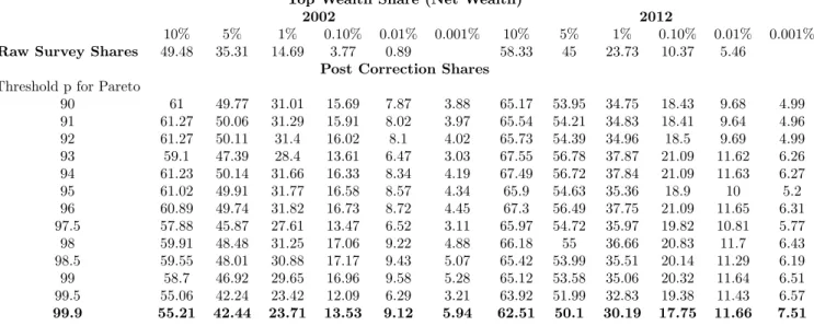
5.1.3 Rich Topping . . . 18
5.2 Representation of Di↵erent Castes by Decile . . . 21
5.2.1 Rural . . . 22
5.2.2 Urban . . . 23
5.2.3 Discussion . . . 24
5.3 Total Wealth Inequality within Caste . . . 24
5.3.1 Top Deciles . . . 25
5.3.2 Lower Deciles . . . 25
5.3.3 Discussion . . . 26
5.4 Total Land Inequality . . . 27
5.4.1 Concentration of Land Within Land-Owning Population . . . 27
5.4.2 Discussion . . . 29 6 Conclusion 29 7 Appendix 33 7.1 A.1 Figures . . . 33 7.2 A.2 Tables . . . 36 7.3 A.3 Methodologies . . . 39 7.3.1 Stratification in NSS AIDIS . . . 39
7.3.2 Converting from Household Level to Individual Level . . . 40
ACKNOWLEDGEMENT
I would like to thank my supervisor Professor Thomas Piketty for being very supportive and open to ideas. He was a constant source of motivation for whole year. Next I would like to thank Professor Abhijit Banerjee for agreeing to be referee. His suggestions were very useful, some of which I was able to incorporate. I would like to thank Lucas Chancel for helping me at crucial junctures by gaining access to datasets without which this data intensive thesis would not have been possible. I extend many thanks to Thomas Blanchet for helping me in technical parts of estimation. I thank Professor Pulak Ghosh for the important datasets which will certainly have a bigger role in my future research.
I thank a lot to Michelle Cherian, Kentaro Asai and Matthias Endres for their help in proof reading my initial drafts of this thesis which played big role in finishing this report on time. Also I thank all my friends and family members for their moral support.
1
Introduction
Economic Inequality has become a major issue in the world. With more and more research in the area using di↵erent datasets, the gloomy picture of an extremely unequal society is becoming explicit, across the world. Almost all the countries have an increasing graph of income and wealth inequality during the recent few decades. It will be too optimistic to shrug it o↵ as a co-incidence. Certainly there are some common factors around the world driving the level of haves and have-nots scenario in society. In this context it is very important to understand di↵erent phenomena which could potentially be the reason behind this. It is further interesting to look at the macro picture to understand why di↵erent countries, despite being in di↵erent development phases, all face an increasing inequality trend.
In the context of global economic inequality, I present the case of wealth inequality in India. I keep the domestic lens of caste active, to not miss the social inequality which might be propelling the uneven distribution of prosperity. I further divide my work here into two sub-topics. First is preparing the long term evolution of wealth inequality series for India. One of the challenges I faced, as any other researcher generally encounters, is the availability of data. A data-driven research carries more weight due to obvious reasons. Fortunately India has a long tradition of wealth surveys. Since 1951, every ten years, all-India surveys are conducted to know the wealth and debt situation in India. These surveys encompass di↵erent physical and financial form of assets. There are some concerns over the quality of data and inter-year comparability- which I have tried to overcome in this paper.
India is a very peculiar country with a complex and regressive caste system. In the study of wealth inequality one can’t ignore this societal peculiarity which is historically older than wealth inequality. Thus, the second sub-topic is understanding economic inequality within the framework of caste. This paper is limited to presenting some simple ranking orders of average wealth and consumption, representing inequality by deciles within the caste-based frame-work (i.e. segregation of castes based on wealth, with higher castes concentrated more in top wealth deciles and lower castes concentrated more in lower deciles). Some may wonder if caste has any relevance today. Unfortunately past unequal distribution of wealth along caste lines has never been corrected. A simple depiction is the land distribution in India. Land forms a major part of wealth in India (Rural India- 65% and Urban India 45%). In the past land distribution was entirely based on caste where the upper-castes of society possessed almost all of the land and lower castes predominantly formed the working class. Colonial period concretized the possessions of land by distributing land titles and land ownership. Indeed, post independence India adopted land reforms aiming for the distribution of land ownership to the real farmers who were mainly from the lower castes. However, even going by the reports of the government this measure has met with partial success and the distribution did not go well beyond certain ranks of the castes. Early adoption of an egalitarian meritocratic system was accompanied by a support system in the form of positive affirmation (reservation/quotas) for the lower castes. The data shows that the situation of every caste has improved over time, but there is no convergence between upper and lower castes. The rate of growth of forward/upper castes in terms of acquiring wealth or consumption is higher than the lower castes. Provided there are positive affirmation policies, one will expect the opposite. It hints towards the harsh reality of ongoing caste-based discrimination in the society.
The paper is structured as follows. Chapter 2 connects this work to the existing literature on wealth inequality. Chapter 3 outlines the various data sets used for the analysis. Chapter 4 presents the evolution of demographics of di↵erent social groups of India since 1901. Chapter 5 presents the evolution of wealth distribution in India since 1961.
2
Literature
This paper produces long term wealth inequality series of India using survey data and correcting the top wealth distri-bution using the Forbes millionaires data. It complements the income inequality series produced by Banerjee (2005) and Chancel and Piketty (2017) on India. The basic approach is similar in terms of utilizing all the available resources to estimate the top wealth and consumption shares. There can be mainly 5 ways to estimate the distribution of wealth as outlined in Alvaredo, Atkinson, and Morelli (2016). First are Household Surveys of personal wealth. Second, the administrative data on individual estates at death. Kumar (2016) uses inheritance tax returns with mortality tables data with an estate multiplier technique to produce top .01% wealth share during 1961-85. Inheritance tax was active during 1953-85. This shows the limitation of this data to study recent wealth inequality. Third is the administrative data on wealth of the living derived from annual wealth taxes. Wealth tax prevailed in India during 1957-2016. The productive assets like shares, mutual funds and securities were exempted from wealth tax. Low collection of taxes and higher costs was one of the reason for its abolition.1 Fourth is the administrative data on investment income,
capitalized to get estimates of underlying wealth. Fifth is the list of rich individuals produced by di↵erent magazines like, Forbes Billionaire’s list. This paper uses Forbes to correct the top share and uses Business Standard millionaire
list for robustness check.
Household surveys are useful to provide information for the bulk of the population, but su↵er from the limitation of not capturing the complete top distribution- either due to non-responses, under-reporting or worse exclusion of the rich (Deaton, 2005; Jayadev, Motiram, and Vakulabharanam, 2007). To emphasize on the issue, I found the combined wealth of top 46 Forbes millionaires in 2012 is 2.5% of the total wealth from nationally representative wealth surveys. Hence I utilize the available Forbes list to correct the top series. In terms of methodology I use the advanced version of standard Pareto interpolation namely Generalized Pareto Interpolation techniques which has been developed in Blanchet, Fournier, and Piketty (2017) and has been used in Piketty, Yang, and Zucman (2017). I contribute in pro-ducing the wealth inequality series since 1960’s. The combined income-consumption-wealth series on Indian inequality will help in analysing the economic inequality from the three prime economic indicators.
The income share of top 10% population shows an increasing trend since 1980 to reach 55% in 2013. Comparing this to wealth share, I find the top 10% share increasing from 45% in 1981 to 58% (pre-correction) and 62% (post-correction) in 2012.
This paper supplements the existing literature Anand and Thampi (2016), Jayadev, Motiram, and Vakulabharanam (2007), and Zacharias and Vakulabharanam (2011) on wealth inequality in India and in other developing countries in general. The methodology adopted here is new and I compare the results from di↵erent methodologies in detail later. The second important point of demarcation is the comprehensive approach undertaken here by visualising wealth inequality not only from economic point of view, but also from social point of view. Gender, Caste and Place of residence are some other dimensions along which inequality has been scrutinized. The main motivation for this comprehensive approach is the peculiar form of Indian inequality where social and economic inequality are weaved together with the thread of caste.
Through this paper, I also add to the existing literature on inequality studies making caste as central social stratifi-cation of the society. Deshpande (2001) argued to make caste as an essential ingredient in the study of stratifistratifi-cation patterns in India’s population and later works Borooah (2005), Thorat (2002), and Zacharias and Vakulabharanam (2011) have highlighted the economic di↵erences among castes which exactly matches with the caste hierarchy present in the society. One extension is through an attempt to disentangle the heterogeneous group of Forward caste2 into
finer categories, Brahmins, Rajputs, Bania and so on. Lack of any caste census in 1931-2010 and as well as lack of caste information from SECC 2011 (Socio-Economic Caste Census) is a big hindrance to any study along caste lines. It will surprise many that there is no concrete population figure of Other Backward Castes (OBC) in India. It is very recently that national representative surveys have started gathering information on castes- which helps in estimating their respective population. I initiated the process of cleaning, sorting and most importantly categorizing the castes. This is a gigantic e↵ort as there are thousands of castes in Indian society with almost no documentation from recent times. I provide basic demographic and socio-economic characteristics for few well known castes. Lack of any prior attempt is an issue to compare the estimated numbers. One robustness check is to compare the estimated population from two completely di↵erent surveys (conducted by di↵erent organizations). I intend to carry out this task, as it has huge potential to analyse the population at finer level. The big social groups - SC, ST, OBC, FC are quite heterogeneous, as detailed later, and hence a finer level analysis will help in policy recommendation on reservations (positive affirmative actions) in India.
This paper also contributes towards the literature dealing with the measure of inequality and polarization in societies-by empirically utilizing the theoretical concepts of representational inequality, sequence inequality and group inequal-ity developed in Jayadev and Reddy (2011) on Indian wealth data. Representational Inequalinequal-ity measures a degree of “segregation” of between di↵erent social groups along any attribute space.3 Sequence Inequality measures the degree
of “clustering” based on hierarchy among social groups. Group Inequality measures the portion of between inequality in the total inequality in a society. I perform Representational Inequality and Sequential Inequality analysis and find the existence of both which has been termed as ordinal polarisation. The population share of all the perceived lower caste groups (SC, ST and OBC) in top decile of wealth and consumption is lower than their overall population share. The situation has deteriorated over the last 40 years. Further a high level of within inequality is found in terms of wealth and consumption which has brief mention in Borooah (2005) also.
2In this paper, I use Forward Caste to denote the Hindu religion population who do not fall under Scheduled Caste (SC), Scheduled
Tribe (ST), Other Backward Castes (OBC). Forward Caste is synonymous to ’General’ class which is used often in India. The basic di↵erence from the point of view of Indian government is that SC, ST and OBC are positively discriminated through reservation/quota in employment and educational institutions.
3
Data
There is neither any all-India level administrative household wealth data nor a caste census data publicly available, which makes the task challenging. Fortunately there are many all-India level large sample surveys to estimate statistics on wealth. Also under demographic particulars in surveys, some information on caste is available. Certainly surveys are not the best in capturing the information perfectly (as some part of the population is ignored. e.g homeless, prisoners etc), but it is the best possible source of information available. In this chapter I will describe in detail the di↵erent datasets I have used. Some datasets (like IHDS) is quite well known and have been well exploited by economists. I will briefly go through such datasets. However, some datasets are less known, like NSS-wealth datasets, which I describe in detail.
Since the study covers a long time period, several rounds of same surveys are used. Since these surveys are supposed to capture the same information, so at di↵erent points, one would expect them to be comparable. Unfortunately, often there are changed definitions, which makes a direct comparison difficult. I have made an e↵ort to make di↵erent rounds of surveys comparable, but it is not possible in some cases. For example, there could be di↵erent type of biases coming from conduction of surveys by di↵erent agencies. One prime example in Indian NSS surveys is that on several occasions half of the sample is surveyed by agencies affiliated to central government and half by state government agencies. Due to di↵erences in availability of resources the e↵orts in surveying can be di↵erent leading to some biases. Due to lack of time, I have not tried to assess such di↵erences and assumed the bias due to such di↵erences to be negligent. This is usually an accepted practice in literature. All other changes which I make are presented below in di↵erent survey blocs.
Since wealth surveys are prone to di↵erential level of under-reporting (with high level of under-reporting coming from land and gold asset holders) and high concentration of wealth distributions at top end, I re-estimate the distribution using the Forbes data (Jayadev, Motiram, and Vakulabharanam, 2007).
3.1
NSS- All India Debt and Investment Survey (AIDIS)
The NSS AIDIS are decennial surveys for the years 1961, 1971, 1981, 1991, 2002 and 2012. It is the primary data source for generating the wealth inequality series. The survey began in 1951 when the RBI (Reserve Bank of India) started All-India Rural Credit Survey with the main objective of identifying the demand and supply of credit in rural India to formulate banking policies and schemes. Information on assets and incidence of debt on rural households were collected to assess the demand side of credit. The next round of survey called All-India Rural Debt and Investment Survey (AIRDIS) was conducted in 1961-1962. This round of survey, for the first time collected details on financial assets, but the survey was still restricted to rural areas. Nationalisation of Banks in 1969 gave a new shift to credit policy, focussing on the hitherto untouched people involved in entrepreneurship, retail trade, professional works etc. and this led to decision to extend the survey to urban areas in the third round of survey in 1971-72. This round also saw an organisational change which brought into place NSSO (National Sample Survey Organisation) to conduct the survey. Unfortunately due to some sampling issues the urban data was never published.
Methodology:
The methodology adopted for the collection of data in NSS AIDIS is di↵erent from the well known NSS consumption surveys. Each selected household is visited twice, once during the first half of the survey period and then during the second half of the survey period. The surveys are conducted during the calendar year for the reference period which matches with agricultural year of the country.4 The asset and liability on a certain fixed date (reference date) is
ascertained. The reference dates are mid-point of the reference period. Depending on di↵erent rounds of surveys, the methodology for ascertaining the asset value changed slightly.
In 1961-62, the asset and liability of the household is derived on a fixed reference date (i.e. 31st Dec 1961 which is mid-point of the reference period July 1961-June 1962) by ascertaining the stock of assets/liabilities as on the date of survey and their transactions/flow during the period of date of reference and the date of survey. In 1971-72 the survey directly collected for the fixed reference date (30th June 1971 and 30th June 1972). In 1981-82, the information on the stock and flow of assets was similar to 1961-62, with changes in valuation.
The details of stratification in di↵erent rounds of surveys are provided in Appendix (Stratification in NSS AIDIS). The important thing to note is that before the 1991 round of survey, households were stratified only on the basis of land possession (primary asset of household wealth). Later research found that the liabilities/debts were not captured properly due to stratification based only on assets. The correction was made from 1991 onwards in the stratification method using land possession and indebtedness status of households in rural areas. For urban areas, monthly per
4For e.g 1961-62 survey collected information from Jan-Dec 1962 for the reference year July 1961-June 1962. Agricultural year in India
is from July to June. Similarly for 1971-72 survey, the survey was conducted during Jan-Dec 1972 for the reference period July 1971-June 1972. And so on for later years of 1981, 1991, 2002 and 2012
capita expenditure and indebtedness status were used.
Assets:
Assets include all items owned by the household which had some money value. The survey has collected the informa-tion on inventory of assets and liabilities on a fixed reference date. The definiinforma-tion of assets has gone through changes in di↵erent years. Physical and Financial assets are the two broad categories. In 1961-62 total assets included the value of 8 di↵erent types of assets- i) Ownership rights in land ii) Special rights in land iii) Buildings iv) Livestock v) Imple-ments, Machinery, Transport Equipments etc vi) Durable household assets (life more than a year and which can’t be purchased at a nominal price) vii) Dues receivables on loans advanced in cash/kind. viii) Financial assets-Government securities, National Plan savings certificates, shares etc. Importantly no information on cash was collected. In 1981-82, Agricultural implements and non-farm machineries including transport equipments were collected separately. How-ever, crops standing in the fields, cash in hand or stock of commodities were not considered as assets. In 1991-92, non-farm business equipments and all transport equipments were collected separately. Unlike previous years there was an e↵ort to collect information on cash in hand of the household. Similar definition and categorization was used in 2002 survey. Bullions and Ornaments were also collected as part of assets. In 2012-13, survey excluded some of the assets which it had collected before. Household durables were excluded on the pretext of valuation concern. Bullions and ornaments were also not collected.
Valuation of Assets:
Estimating the total wealth requires not only the number/amount of assets but also their valuation. In 1961-62, all the values of the physical assets were evaluated using the fixed average market value prevalent at the time of the first round of the survey. Dues receivables were evaluated using average wholesale prices. Shares were valued at their paid-up value and all other financial assets were evaluated at their face values. There was a slight change in 1981-82 in the valuation. The value of physical assets owned on the reference date was simply the value on the date of survey minus the value of transaction between the reference date and the date of survey. Essentially it means di↵erent prices for the same assets were used.
Due to the lack of book value for valuation of assets for household sector, the following procedure is followed: i) Value of physical asset acquired prior to the 30th June 1981 (1991, 2001, 2011) was evaluated in its existing condition at the current market price prevailing in the locality on the date of survey if the asset is owned on the date of survey or on the date of disposal if the asset is disposed of during the reference period in a manner other than sale.
ii) In case the asset is sold/purchased during the reference period, sale/cost price is considered as value of the asset. If the asset is acquired by way of construction, the expenditure incurred on construction is taken as its value. iii)If the asset is acquired other than purchase, then the value of the asset in its existing condition as prevailing in the locality at the time of acquisition is noted. iv) If the asset is acquired during the reference period and is also disposed of during the said period, the disposal value is reported
Availability of the data: Micro-individual survey files are available for the last three rounds of survey- 1991-92, 2002-03 and 2012-13. For previous surveys, only source of information is annual reports. The 1981-82 and 1971-72 reports are available5. The 1961-62 report is not digitised yet and is available in hard copy format.6 The samples are
fairly big in size and vary for di↵erent years. The assets are collected at household level in all the surveys. I decided to work with individual level wealth as it provides a better understanding of wealth distribution from the perspective of inequality study. For example, a statement like top 10% of the households own 50% of wealth is a weaker statement to make in studying inequality if those 10% happened to represent 50% of total population. Household level inequal-ity hides the per-capita level information, which is better suited for inequalinequal-ity statistics. Since there is no standard method to divide the wealth within household, I equally split among adult household. This will hold true for most of the physical wealth (like land, building, transport etc) which is synonymous to public goods within household. This procedure allows global comparison of inequality statistics. Equal split within a household is a big assumption in Indian society- where women usually do not own wealth because of various reasons like customary transfer of wealth from father to son, biased gender inheritance laws7 and general gender discrimination in India, but usually have a say
(even if unequal) in managing at the household level. The social norm of primogeniture also leads to unequal share of wealth - major share of inheritance going to the eldest son. The definition of adult population is chosen as (> 20 years) for all the analysis.
In all the analysis related to wealth using AIDIS datasets, adult individual is the basic unit of reference. One of the issue is that the tabulated data for surveys are provided at household level. For converting the wealth values at individual level, I use decadal growth rate of household adult size from next round surveys, for which micro-data is available. The decadal rate of change in HH adult size in 1991-2001 is assumed to be same in 1981-1991 by decile.
5http://www.mospi.gov.in/download-reports
6The library of College of Agriculture Banking, Pune, has the report and it is accessible on prior appointments. 7Before Hindu Succession Amendment Act 2005, women were deprived of inheriting land and other properties.
I use a correction factor- to make the estimated data consistent at macro level population. Full detail is given in Appendix “Converting from Household Level to Individual Level”.
Justification for using total wealth instead of net wealth Further the distribution is estimated with household per capita total wealth and not with household per capita net wealth. Net wealth is total household wealth minus total household debt. The debt level from AIDIS are suspected to be unreliable due to reasons of strong tendency of under-reporting of liability, issues related to sampling methodology and relative increase in state sample compared to centre sample Chavan (2008) and Narayanan (1988). Comparing the debts handed out by commercial banks, cooperatives and other lending agencies,Gothoskar (1988) found under-estimation of 40% in 1971-72 round and 50% in 1981-82 round. The other reason to use total wealth is that for pre-1991 surveys the information is only available in tabulated form which restricts estimation of distribution of net wealth as the classification is by total asset ownership and not by net wealth status (Subramanian and Jayaraj, 2008). Due to these issues, I work with household total assets instead of household net assets.
3.2
IHDS- Indian Human Development Survey
IHDS - is a nationally representative panel survey for the years 2005 and 2011. It is a joint venture of University of Maryland and National Council of Applied Economic Research (NCAER). The survey collects information on income which is not captured in other household surveys in India.Further it provides information on Brahmin caste- a sub-group within Forward caste- which is unavailable in NSS surveys. This paper uses the cross-sectional aspect of the dataset8 for two purposes.
First to produce general socio-economic characteristics of di↵erent castes in India and perform a comparative analysis using the latest round of survey- IHDS 2011-12.9. The survey sampled 42,152 households with 2,04,568 individuals
interviewing the head of the household to get this information. I create caste group based on religion and caste codes based on the following combination- a) Dalits (SC), Adivasis (ST) and OBC’s (Other Backward Castes)are coded as they are, regardless of their religion; b) Next Brahmins are coded as Brahmins. c) Next all Hindus10 who are not
categorized above are coded as Forward Caste (FC); d) Next, all the Muslims, who are not yet coded are coded as Muslims. e) All the rest of the population is grouped as Others.
I would like to highlight that this classification is di↵erent from the one given in IHDS. I chose this categoriza-tion, since SC, ST and OBC have some provisions of positive discrimination11 from central and state governments
which directly impacts the educational and income outcomes.
4
Demographic Profile
India is the second most populous country after China and 7th largest in terms of area. India is full of diversity.
India has 29 states with 1.3 billion population. The largest state of India has more than three times the population of France. It is one of the oldest civilisations in the world, and is the birth place of four existing religions of the world- Hinduism, Buddhism, Jainism and Sikhism. It also has the third largest Muslim population in the world. There are 22 national languages and a caste system with ⇠ 4000 castes. Religion, race, caste and language not only determine personal identity but also play an important role in many economic decisions, both at household level and at national level. It became a secular, democratic country and adopted a socialistic pattern of production after becoming an independent nation in 1947 and is now transitioning towards a capitalist system. All these demo-graphic, social, political and economic factors have some contribution towards the existing “Indian form” of inequality.
This chapter outlines the evolution of basic demographic profile of India in 1901-2011. The hundred years time period provides a long term evolution of population structure. Understanding of inequality in India will be incomplete without taking into account its societal structure. The demographic patterns across di↵erent religion and social groups are estimated using survey data and the Census. Census was started in India in a regular manner from 1881 onwards. One has to be cautious while looking at the data from the pre-independence era. The British territory has seen a gradual expansion in India and some of the di↵erences in population is due to di↵erent areas mapped under Census.
8I intend to use the panel structure of the dataset in my future research on understanding the evolution of di↵erent economic outcomes
for di↵erent castes
9I refer IHDS 2011 in the whole document. The survey was conducted between Nov 2011-Oct 2012 10There are 5 major religions in India-Hinduism, Islamism, Christianism, Buddhism, Sikhism
11usually termed as reservation in India- as 15%,7.5% and 27% of total seats are reserved for SC, ST and OBC respectively in all the
government educational institutions and government employment positions. SC, ST and OBC are sometimes also referred as reserved castes.
The first attempt of conducting the census was between 1840-65 and it covered only the three big cities of that time-Bombay, Madras and Calcutta. Later at the time of independence of India in 1947, India was partitioned and two nations were formed out of it. The partition was along religious lines and resulted in a change of the population mix in terms of religion.
The total population of India grew from 253.9 million in 1881 to 1210.7 million in 2011. As per Thomson-Notestein-Blacker classical demographic transition, India was in Pre-transitional phase of very high crude birth rate (CBR) and crude death rate (CDR) at > 40 per thousand till 1920, and the population was almost stable. The small increasing population of Census data is mainly on account of increasing covered area. India entered into second phase of the Transition in 1920. The CDR started falling after 1920 but the CBR remained high till 1960’s. The gap between CBR and CDR resulted in population growth. The life expectancy also increased from less than 20 years in 1911-20 to over 40 years during 1951-60. The decline in CBR started from 1960’s (start of Middle transitional phase) and it dropped to 22.1 in 2011. The total fertility rate (TFR) reached just above replacement level at 2.4 in 2011. The period during 1970-2011, saw a consistent decline in CBR, but the di↵erence between CBR and CDR resulted in population explosion during this phase. Now India is considered to be in the Late Transitional phase, where CDR has stabilised and CBR/TFR is continuously declining. The population of the country has increased 3.35 times its population in 1951. The rate of growth was lowest in 1921 and accelerated after 1951 with decadal increase of 20% during 1961-2001. It is only in last census decade that the rate of growth has declined to 17.7%
4.1
Population Share- Rural Urban divide
The urbanisation level in India has grown from a level of 10.8% in 1901 to 31.2% in 2011. It is still a rural dominated country and the urbanization level is much lower than what is experienced in developed countries. France US, UK all have urbanization level as high as 80%. The urbanization level is very low even compared to developing nations like-China (55%) South Africa (65%), Russia (74%). It is even lower than the urbanisation level in partitioned countries-Pakistan (38%), Bangladesh (34.3%). India still is a country of villages where more than 65% of the population resides. Table 1 provides the evolution of urban population share in the country in long run.
Table 1: Rural Urban Population Share
Census Year 1901 1911 1921 1931 1941 1951 1961 1971 1981 1991 2001 2011 Population % Rural 89.16 89.71 88.82 88.01 86.14 82.71 82.03 80.09 76.66 74.28 72.17 68.84 Urban 10.84 10.29 11.18 11.99 13.86 17.29 17.97 19.91 23.34 25.71 27.81 31.16
Source:Census data.
The share of Rural and Urban population in NSS consumption survey in 1983-2009 is provided in Fig. 11. We can notice a slight di↵erence from the census figures. Urban area is slightly over-represented in the data. The definition of Urban area is the same as used in Census.12
4.2
Population Share by Religion
India has residents from all the religions. Islam and Christianity are imported religions to India and Buddhism, Jainism and Sikhism have their origin in India. The above mentioned 6 religions, makes up for more than 99% of Indian population Hindus are in majority in the country. One important remark on aboriginals or people from Schedule Tribe (ST) populations in the country is that before the census, they were categorized separately from Hindus. Post independence they are clubbed under Hindus. The estimate of ST population is provided later. They are captured in the census under Hindu religion. The population proportion is almost constant except a decline in Hindus share and increase in Muslims share.
Table 2: Religion-wise Population Share
Religion Census Years
1840-65 1860-69 1867-76 1881 1891 1901 1911 1921 1931 1941 1951 1961 1971 1981 1991 2001 2011 Aboriginals 0 0 0.28 2.53 3.23 2.92 3.28 3.09 2.36 6.58 Hindus 71.67 75.96 72.93 74.02 72.32 70.37 69.4 68.56 68.24 65.93 84.1 83.45 82.7 82.3 81.53 80.5 79.8 Muslims 19.08 16.31 21.39 19.74 19.96 21.22 21.26 21.74 22.16 23.81 9.8 10.69 11.2 11.8 12.61 13.43 14.23 Christians 5.36 0.51 0.47 0.73 0.8 0.99 1.24 1.5 1.8 1.63 2.3 2.44 2.6 2.44 2.32 2.34 2.3 Sikhs 0 1.1 0.61 0.73 0.66 0.75 0.96 1.02 1.24 1.47 1.79 1.79 1.9 1.92 1.94 1.87 1.72 Others 3.9 6.13 4.32 2.24 3.03 3.75 3.87 4.08 4.21 0.57 2.01 1.63 1.6 1.59 1.6 1.86 1.95 Total % 100 100 100 100 100 100 100 100 100 100 100 100 100 100 100 100 100
Total Population (mill) 1.7 103.1 191.1 253.9 287.2 294.4 313.5 316.1 350.5 386.7 361.1 439.2 548.2 683.3 846.4 1028.7 1210.7 Source:http://dsal.uchicago.edu/copyright.html.
12The definition of Urban area depends on 3 criteria namely- 1) Population threshold (¿5000) and density (400 sq.km) 2 Proportion of
4.3
Population Share by Caste
Define caste: Caste is a system prevalent in India society which can be thought of as a practised version of varna system enumerated in religious scriptures. There is enormous literature on caste in sociology and anthropology (Kannabiran, 2009). I will describe certain essential components of caste system which still have relevance today. I define in detail some features of the caste system.
First- Caste system is not only a Hindu religion phenomena anymore though it indeed has its beginning in Hin-duism/Brahmanism way of living. It has now entered into all the religions in India, in one or other form. It is believed that Buddhism and Jainism, the two ancient religions of India were born in around 5th century B.C against the backdrop of high levels of social inequality that generated from discriminatory norms of Brahmanism of that time. With time these religions themselves acquired the prejudiced traits of Brahmanism. The decline of Buddhism in its own birthplace is often associated to this reason.
Second- caste system is not varna system. Varna system has 4 (or 5) categories namely Brahman (priests, scholars and teachers), Kshatriya (rulers, warriors and administrators), Vaishya (agriculturists, merchants) and Shudra (work-ers / small farm(work-ers / service provid(work-ers), and it has its origin in Dharamshastras13. The fifth category consisted of
Untouchables. The first three categories were allowed to wear the sacred thread and study religious texts. Even though caste system is believed to have come from varna system, both of them are not identical. Today society associates more with caste (or jatis in Hindi), which are thousands in numbers and vary regionally. (Srinivas, 1955) says that these thousands of castes can be clustered around varnas. This makes comprehension easier.
Third- Caste system has broad acceptance in the society. It is not a menace in the opinions of majority of the population. It acts as an identity and beyond that it provides some of the benefits which the welfare state provides (Srinivas 2004). For all the practical purposes, there is very less competition inside this system to outrank others, because caste is determined by birth. The topmost rank is reserved forever for the perceived creators of the system -Brahmans.
Fourth- Caste system provides a form of social status to every caste. Indeed, as with any form of status, it comes at some cost. Some castes derive higher status tag at the expense to lower status tag to others. However, it is more generous in the sense that the higher status has been distributed to fairly large proportion of population. 5% Brahmins and around 5-7% Rajputs (from Kshatriya of varna), Bania ( 2%) are considered higher castes. It could be surmised that the most important and unique factor which provides sturdiness to the caste system is the fact that it assigns relative position to every caste in the society. Even though Rajputs come second in hierarchy, they are on top of 90% of the population. Similarly Banias derives utility by being higher in status to 88% of the population. And this way the caste system has created a situation where all the castes (except the ones at bottom) derive some kind of superior social status compared to other castes.
Overall the debate on caste system has remained contentious. The most famous debate in recent history is the Gandhi-Ambedkar debate on caste. Gandhi (considered as father of the nation) was against the discriminatory na-ture of caste system. He coined the term Harijans (in Hindi it means-children of God) for untouchables and worked throughout his life for their upliftment. However, he was not against the caste system itself. According to him, division of labour is inevitable in society and there was no need to overthrow the caste system which was based on division of labour. On the other hand, B. R. Ambedkar (architect of Indian Constitution) was against the stratification of society based on caste. He made a distinction between division of labour and division of labourers, where the first one is choice-based and the later imposed by the caste system. He said that outcaste is a product of caste and unless caste system is uprooted from its base, the discrimination based on caste will remain. Hence he demanded complete overthrowing of the system. In principle, I would agree with the Ambedkar stance on the caste system, however one cannot ignore the reality of the society. The difficulty to overthrow the system is its huge approval in society. One of the peculiar aspects of the caste system, which has become the strongest pillar of its existence, is caste endogamy. Everyone is supposed to marry within one’s own caste. This paper finds strong evidence of caste homogamy in the society, where 94% of total marriages are within-caste marriages.
Caste became part of census in full fledged manner in 1901 census. The historical census data at caste level is available online at Digital South Asia Library (University of Chicago)14. Table 3 provides top 20 castes which existed
in 1901 and 1911.15The last census which gathered caste data and is available in public was in 1931. Indian government wanted to stop caste-based census due to the fear of re-enforcing the caste identity. However provision of affirmative
13Manusmriti- the first one to be translated in English by Britishers in 1784 to rule Hindus in India. I wonder the impact of this colonial
act in reinforcement of caste system in the form it is today.
14http://dsal.uchicago.edu/copyright.html
actions were made for Scheduled castes (Dalits) and Scheduled Tribes (ST) since 1951. Scheduled caste (SC) was not a single caste entity but a list of castes. The people belonging to castes in SC were considered untouchables during that time. They formed the lowest rung in the caste hierarchy. For the implementation of the clauses of positive affirmation enshrined in the constitution, census gathered information on SC and ST. Later in 1990, India extended the caste-based positive affirmative actions (also referred as reservation policies) for Other Socio-Economic Backward Class of the society. These are the population often coming from Other Backward Castes (OBC) castes. Again OBC is not a single caste but a list of thousands of castes. When the reservation policies was promulgated for OBC’s, there was a major problem in estimating the population of OBC’s, because there was no census information. OBC population was estimated from 1931 census using the population growth. Facing the problem of lack of information on castes, Indian government conducted the Socio-Economic Caste Census in 2011 to update the knowledge on di↵erent castes. However, unfortunately the data has not been made public.
Table 3: Population Share - Census
1901 1911
Caste Population Size Population %age Caste Population Size Population %age Shekh 28,708,706 9.16 Sheikh 32,131,342 10.25 Brahman 14,893,258 4.75 Brahman 14,598,708 4.66 Chamar 11,137,362 3.55 Chamar 11,493,733 3.67 Ahir 9,806,475 3.13 Ahir 9,508,486 3.03 Rajput 9,712,156 3.1 Rajput 9,430,095 3.01 Jat 7,086,098 2.26 Burmese 7,644,310 2.44 Burmese 6,511,703 2.08 Jat 6,964,286 2.22 Maratha 5,009,024 1.6 Maratha 5,087,436 1.62 Teli and Tili 4,025,660 1.28 Kunbi 4,512,737 1.44 Kurmi 3,873,560 1.24 Teli and Tili 4,233,250 1.35 Kunbi 3,704,576 1.18 Pathan 3,796,816 1.21 Pathan 3,404,701 1.09 Kurmi 3,735,651 1.19 Kumhar 3,376,318 1.08 Kumhar 3,424,815 1.09 Kapu 3,070,206 0.98 Kapu 3,361,621 1.07 Napit 2,958,722 0.94 Mahar 3,342,680 1.07 Mahar 2,928,666 0.93 Koli 3,171,978 1.01 Jolaha 2,907,687 0.93 Hajjam 3,013,399 0.96 Bania 2,898,126 0.92 Lingayat 2,976,293 0.95 Kaibartha 2,694,329 0.86 Gond 2,917,950 0.93 Lingait 2,612,346 0.83 Jolaha 2,858,399 0.91 Koli 2,574,213 0.82 Palli 2,828,792 0.9 Source:http://dsal.uchicago.edu/copyright.html.
As per Census data16the proportion of SC in population has increased from 14.67% in 1961 to 16.6% in 2011. During
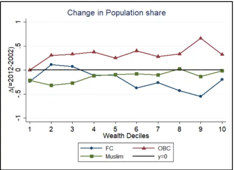
the same time period the proportion of ST has increased from 6.23% to 8.6%. Apart from natural growth rate of SC and ST, classification of more castes/tribes into SC/ST17 has contributed in the increase of their population share. Apart from the Census, surveys too provide valuable information on the estimates of population. The Census is conducted once in 10 years and the NSS consumption surveys are conducted almost every 5 years. Hence NSS surveys in a way complement the Census and can be utilised to study mid-year variations in the population profile. Post 1999 NSS surveys allow the breakdown of the population into OBC also. I categorize the population based on a combination of religion and caste which has been mentioned in a section of the IHDS dataset. The same definition has been used in NSS also.18 Fig. 1a depicts the evolution of population share of SC, ST, OBC and FC since 1983. We can see that
SC and ST are slightly over-represented in the survey (SC- 20% and ST -10%). We also observe an increasing share of OBC population share and corresponding decreasing share in population of FC. Non-Hindu population share declined in 1999, because of the creation of the OBC category. OBC Muslims are categorized under OBC.
16http://censusindia.gov.in/
17The recent most addition is in 2015. http://pib.nic.in/newsite/PrintRelease.aspx?relid=115783
181. SC(Scheduled Caste) 2. ST(Scheduled Tribe) 3. OBC(Other Backward Castes) 4. FC(Forward Castes-Hindus who are not
Figure 1: Population Share from NSS
(a) Proportion of SC/ST/OBC/FC (b) Share of Hindu in di↵erent castes
The share of di↵erent caste groups in Rural, Urban sector separately is provided in appendix Fig. 12. We observe that FC community is disproportionately concentrated in Urban areas and STs are mainly confined to Rural areas.
The second subgraph 1b shows the proportion of Hindus in SC, ST and OBC. It is important to re-iterate here that SC, ST, OBC which are reserved communities in India (with positive affirmation) are not restricted to just the Hindu population. Caste has intruded into other religions also. We see an increase of other-religions in ST and OBC. In 1983, Hindus comprised almost 90% of ST which dropped to 86% in 2009, whereas for the OBC the share of Hindu population dropped from 88% to 84%.
IHDS datasets allows to split FC category into Brahmins and rest of the FC, which help in estimating the popu-lation share of Brahmins (⇠ 4.86%) and some of their general demographic and socio-economic characteristics. Table 13 provides the percentage of population in di↵erent caste groups. The information on Brahmin community which is considered as the highest caste in the caste hierarchy makes this table interesting. As there is no census on castes, surveys are the only source to gauge their population share or other characteristics. Another important observation is that child and young population among SC, ST and OBC is higher than their respective population, whereas adult and old population of FC is higher. This hints towards decreasing fertility level of FC.
Another nationally representative dataset namely, NFHS(National and Family Health Survey) allows to further split the FC into di↵erent castes.19 Table 14 provides the population shares. I split FC into Brahmins (4.7%), Rajputs
(proxy for Kshatriya- including Marathas 4.9%), Bania (2.1%), Kayasth (.6%) and Others (9.3%). The population share of Brahmins here is close to what we get from IHDS dataset- which is a good sign for the categorization. The observation on fertility holds for other FC groups too. They have higher proportion of adults and are older compared to their overall population share.20
Comparing with 1901,1911 Census we see almost same proportion of Brahmins after almost 100 years! Rajput+Maratha population proportion is also very close to what it was a century ago. Bania population is higher in NFHS, but it could simply be due to categorization of more castes into this category. Business as a profession has been adopted by other castes and those castes have now been associated with Bania community.
The next few figures in the Appendix (13 and 14 show the proportion of SC/ST/OBC in di↵erent religions in surveys. Pre-1993 surveys have no categorisation such as the OBC. In Hindus the share of SC and ST is almost stable at around 9.5% and 19-21% respectively and they are slightly over-represented in the survey compared to Census estimation. For later rounds we see in 1999, OBC’s formed 38%, 30%, 20%,13.6% in Hindu, Muslims, Christians and Sikhs respectively which increased to 43%,43%,25%,21% in 2009 in the same order. The increase in OBC population is in all religion which is chiefly is due to reclassification of more castes into OBC. The potential demographic reasons like - growth rate, migration etc. usually would take longer time to translate into such big changes.
19Currently the categorization is based on google searches, crowdsourcing etc. It is prone to biases and hence I am working on basing
these categorization on some historical authentic sources.
4.4
Economic Characteristics of di↵erent Castes
IHDS and NFHS datasets are utilized to compare the socio-economic characteristics of di↵erent castes. IHDS datasets has the additional benefit of being a panel dataset to understand changing conditions over 20 years. Also it is the only dataset which captures income. I intend to perform a panel data analysis in my future research. However, for the purpose of this paper, I restrict my anaysis to a cross-sectional one.
4.4.1 Economic Aspects
Table 4 shows the mean values of basic economic and educational characteristics of di↵erent caste groups. The values are given at both household and per-capita level. It provides a clear picture of stratification in the society. The second last column “Others” contains the rest of the population which belongs to the Non-Hindu, Non-Muslim religion group and does not fall under SC/ST/OBC. This is a rich minority cluster (with only⇠ 1.5% population) in terms of all the economic and educational parameters. The last column shows the all-India statistics.
Income: Average annual income of an household in India is Rs.113,222(Rs.⇠ 9, 435 per month). The annual income of ST and SC group stands at 0.7 times and 0.8 times lower than the all-India average income. OBC and Muslims both have around 0.9 times household income of the overall average income. Forward castes (FC), have average household income at 1.4 times the all-India income (with a slight di↵erence between Brahmin and Non-Brahmin). There is sequential inequality (SI) based on average income with ranking ST < SC < M uslim < OBC < OVERALL < F C(N on Brahmin) < F C(Brahmin) < Others trend. We see a similar trend at per-capita level of annual in-come. The standard deviation which is not present in this table is highest for Others followed by FC(Non-Brahmin), FC(Brahmin), SC, Muslim, OBC and ST.
Wealth: Wealth/Assets in IHDS is simply the average of indicator (=1) of the presence of for 33 di↵erent household durable goods like TV, Air Conditioning , 4-wheeler etc. It has a range of 0-33 and is defined at HH Level. The SI based on assets across di↵erent caste groups is visible with ranking ST < SC < M uslim < OVERALL < OBC < F C(N on Brahmin) < F C(Brahmin) < Others, which is similar to income trends.
Consumption: The consumption data shows similar pattern with OBC and Muslim groups near the all-India average, SC and ST below average and both Brahmins and non-Brahmins performing better.
Table 4: Wealth,Income and Consumption Mean Values-IHDS 2011
SC ST OBC FC(Brahmin) FC(Non-Brahmin) Muslim Others OVERALL Annual Income of HH (in Rs) 89,356 75,216 104,099 167,013 164,633 105,538 242,708 113,222 Per Capita Annual Income (in Rs) 19,032 16,401 21,546 35,303 36,060 20,046 56,048 23,798 Annual Consumption of HH (in Rs) 87,985 72,732 108,722 146,037 143,497 102,797 181,546 109,216 Per Capita Annual Consumption (in Rs) 18,740 15,860 22,503 30,869 31,430 19,525 41,924 22,956 ASSETS 12.7 10.2 14.7 18.2 17.9 13.3 22.2 14.6 ASSETS2005 12.2 9.9 14.2 17.5 17.1 12.9 21.2 14.1 Highest Adult Education 6.7 5.9 7.8 11.5 10.3 6.6 11.6 8.0
Highest Male Education 6.3 5.6 7.5 11.3 9.9 6.0 10.5 7.6 Highest Female Education 3.9 3.3 5.0 8.6 7.8 4.6 10.0 5.3
Source:Author’s calculation using NFHS IHDS 2011 datasets.Design weights are used to estimate these values.
Using NFHS 2005, we can compare between more caste groups in FC. Table 16 in Appendix presents the wealth index provided in the dataset, categorizing the population in 5 brackets from Poorest to Richest. We see that 50% of the Brahmin, 31% of Rajputs, 44% of Bania and 57% of Kayasth fall in richest category. For other caste groups only 5% ST, 10% SC,16% OBC,17% Muslims fall in richest category.
I find a high level of sequential inequality in society, which implies clustering of social groups. FC is clustered more towards higher income/consumption/wealth values. OBC and Muslims are in the middle and SC/ST cluster towards the lower end. This clustering of di↵erent groups is parallel to the caste hierarchy with FC the highest caste and SC/ST the lowest in hierarchy. Economic ranking follows caste hierarchy, making caste a valid stratification in the society. It is important to keep in mind that the standard deviation is also very high in FC groups, i.e. not all are well o↵ in that group. The clustering of social groups in not perfect.
4.4.2 Education
The last three rows of Table 4 depict the highest level of education for adults, males and females among di↵erent caste groups.21 Brahmins have highest adult education followed by Others and FC (Non-Brahmins). The
com-parison for adult education across di↵erent community gives- ST < M uslim < SC < OVERALL < OBC < F C(N on Brahmin) < F C(Brahmin) < Others The di↵erence between Brahmin and ST is 5.6 years, Brahmin and Muslims is 4.9 years, Brahmin and SC is 4.8 years, Brahmin and OBC is 3.7 years and Brahmin and Other FC is 1.2
years. Muslims who are almost near the overall average in economic parameters fall behind the SC group in terms of education.
Taking note of the highest male and highest female education pattern separately, we observe same trend among caste groups as we saw for the highest level of adult education. This shows the di↵erent trajectory of education curves among di↵erent caste groups. Another important point to note is that among all the social groups, women have lower mean education than men. There is a secular gender discrimination in the society. This shows a di↵erent trajec-tory of education curves between men and women in every social group. The interaction of di↵erent trajectories of education curves among social groups and among sexes are potentially a crucial determinant in shaping up inter-caste and inter-religion marriages. I explore this in detail in chapter on Assortative matching.Comparing among females, FC (Brahmins and non-Brahmin) communities have the highest average years of education, implying these caste groups are sending more of their girls towards schools and colleges.
Using NFHS 2005 I compare the education level of adult in other Forward castes [Appendix Table 17]. Kayasth with 12.3 years of education is highest, followed by Brahmins (11.9years), Bania (10.3 years), Rest of FC(9.16yrs) and Rajput (9.05 years). The qualitative comparison is same as found in IHDS datasets, though there is slight change in average years of education.
Within SC/ST/OBC Analysis: I look within the SC/ST/OBC category to see if there are di↵erences across di↵erent religion groups. The table 5 presents the relative performance of the groups with respect to all-India average values. We can see that within ST, Christians have 1.6 times income and assets than all-India average and their educational level is better than many other groups. Muslim ST’s economic parameters are closer to all-India average but education wise they are behind. Hindus and Other/No religion ST’s which forms 78% and 12% of all ST’s are the worst performing groups.
In the SC group, Hindu (93%) and Others (6%) are two major groups and we see that SC’s from other religions have outcomes at par with the all-India level. Hindu SC’s have worse outcomes and their mean assets have declined from 2005, which is a worrying issue.
In OBC, the two big groups are Hindu (82%) and Muslim (16%). Hindu OBC’s have better educational averages than Muslim OBC’s. On the economic scale they look almost the same. The small group of other religion in OBC’s are in no way backward.
Table 5: Within SC/ST/OBC Relative to all-India: IHDS 2011
ST SC OBC
Hindu ST Muslim ST Christian ST Others ST Hindu SC Muslim SC Others SC Hindu OBC Muslim OBC Others OBC Annual Mean Income of HH (in Rs) 0.58 0.97 1.6 0.54 0.78 0.81 0.9 0.91 0.88 1.38 Per Capita Mean Annual Income (in Rs) 0.58 0.86 1.69 0.67 0.78 0.75 0.97 0.92 0.74 1.51 Annual Mean Consumption of HH (in Rs) 0.63 1.27 1.29 0.44 0.8 0.99 0.86 0.97 1.09 1.26 Per Capita Mean Annual Consumption (in Rs) 0.64 1.12 1.37 0.55 0.8 0.92 0.93 0.98 0.92 1.39 ASSETS -4.9 -1.21 1.71 -5.82 -2.2 -1.08 0.9 -0.08 0.43 4.9 ASSETS2005 -4.66 -1.07 1.39 -5.46 -2.1 -0.88 0.85 -0.09 0.46 4.48 Highest Adult Education -2.36 -1.41 1.8 -2.99 -1.41 -2.13 0.25 -0.08 -1.13 2.05 Highest Male Education -2.19 -0.48 1.68 -2.98 -1.35 -2.26 -0.22 0.07 -1.2 1.48 Highest Female Education -2.3 -1.24 2.4 -2.86 -1.51 -1.18 0.73 -0.28 -1 3.07
5
Wealth Inequality Series
This chapter illustrates the distribution of wealth among households in India. Instead of using gini coefficient as a single measure of inequality, the emphasis is on estimating di↵erent shares of wealth in top 10%, middle 40% and bot-tom 50% of the population (Piketty, 2014). This distribution of wealth is also examined among di↵erent caste groups. Previous chapter has already established the stratification in society along castes from simple economic parameters. In this chapter, the focus is entirely on wealth, which is associated with welfare, a tool for consumption smoothing, a source of power and contribution in total income through asset income (rent). Micro-files allow for more detailed analysis, like age and education profile of di↵erent strata of the society.
I have made an e↵ort to look into the issue of wealth inequality from social point of view. Distribution of land is analysed in detail. Land happens to be the most important asset of Indian households in monetary value. India has tried in the past to achieve an equitable distribution of land with various land reform measures.22 Today the slogan of
“land to the tiller” has died down in India partly due to decline in the number of big land sizes (population explosion has a major role in division of land plots, long drawn court cases by landowners to stall the land reforms etc.) and partly because of arrival of new opportunities in manufacturing and service sectors. Unless India develops di↵erent
forms of assets, the issue of unequal distribution of land can’t be neglected. The distribution of wealth in di↵erent social/caste groups has been studied with an attempt to characterize the evolution of the pattern. Representational Inequality-i.e. lower presence of a certain caste group than its proportionate share in the population has been exploited in Section 5.2 , apart from the top share statistics. Both across-castes and within-caste inequality have been examined in detail. The dichotomy between rural and urban sectors has been highlighted across all the outcomes.
The methodology in estimating the top share is still new and evolving. The limitation of surveys in capturing top wealth holders is dealt in two ways- 1)By using Forbes millionaires data and making an assumption of Pareto distribution at top percentiles.(Blanchet, 2016; Garbinti, Goupille-Lebret, and Piketty, 2017) 2) A novel attempt to re-estimate the inequality in selected urban areas23.
The results are accompanied by discussions which is an attempt to look for the reasons in past and current government’s economic and social policies. The trends and evolution has been analyzed in detail. The discussions part in every section mentions potential future research.
The chapter begins with providing a description of the contribution of di↵erent assets in the total household wealth at all-India, Rural and Urban sector separately (Table 6).
Table 6: Contribution of di↵erent assets in total Wealth
Contribution of Di↵erent Assets in Wealth (excluding Durable HH’s)
Rural Urban All-India
Type of Assets/Year 1961 1971 1981 1991 2002 2012 1981 1991 2002 2012 1981 1991 2002 2012 Land 66.49 69.92 66.92 68.12 65.00 69.84 38.21 40.04 41.62 45.26 60.06 59.33 56.59 56.36 Building 22.52 18.76 22.31 22.69 24.28 20.33 41.98 44.34 40.92 43.24 27.00 29.47 30.26 32.89 Livestock 8.00 6.81 5.39 3.58 4.35 1.55 0.94 0.48 0.47 0.10 4.33 2.61 2.95 0.75 Agricultural Machinery,
Equipments and Transportation 2.99 2.83 3.99 3.99 3.99 2.70 5.90 5.36 6.76 3.17 4.44 4.42 4.99 2.96 Financial Assets - 1.15 1.29 1.56 2.28 5.46 12.50 9.30 9.94 7.96 3.97 3.98 5.03 6.83 Loan Receivables 0.52 0.11 0.06 0.10 0.12 0.47 0.49 0.29 0.28 0.19 0.19 0.17 0.21
Looking at all-India verticals, we see that Land value share is the highest but is on a gradual declining trend. The share has declined from 60% in 1981 to 56% in 2012. Rural sector expectedly has land as the most valued asset and it has almost remained at around 67%± 3% since 1961. This hints towards continued existence of lower material wealth in rural sector. In Urban sector, land share is lower than all-India level but it shows an increasing trend from 38% in 1981 to 45% in 2012.
Building is the second most important asset in the wealth. It is surprising to note that Land and Building together form 90% of the total household wealth. The decline in land share is accompanied by increase in the Building value share. In Rural area, the share of building has hovered around 20%± 2% except in 2002 when it is at 24%. The rural village morphology allots only a small share of land area towards living and common space24Most of the land is dedicated to cultivation. In Urban area, building share is almost double than that of rural area at around 42%± 2%. The stagnancy in the building share might look surprising as in many cities the advancement of apartment culture is accompanied by high rise in building prices. One possible explanation is almost equivalent increase in land prices which has not let the building share in total wealth rise.
Financial Assets has the third largest share and it has increased to almost 7% level in 2012 from 4% in 1981. This is in contrast to high level of financial assets in developed countries. For example in France and US the share of financial assets stood at 30.9% and 48.3% in 1979.25. There is a declining trend in the share of financial assets in
Urban areas which is surprising. To some extent the decline can be explained by the change of definition of financial assets (explained in data section) in di↵erent rounds of survey. Non-reporting/non-inclusion of rich households could be another potential reason.
The supremacy of physical assets over financial assets is undoubted. Financial assets is a very small small part of total household wealth.
Agriculture Machinery, Non-Farm Machinery and Transport Equipements comes next in the descending list of con-tribution to total wealth. It’s share has declined from 4.4% in 1981 to 2.96% at country level. In Rural area this component remained stable at almost 4% for 3 decades before dropping to 2.7% in last survey. Urban area, has seen a decline from 5.36% to 3.17%.
Livestock used to be around 3-4% of total wealth till 2002 before dropping to 0.75% in 2012. This decline is solely attributed to Rural areas where we see a decline of 3 percentage points. Interestingly in 1961, the share of livestock was more than the share of financial assets in 2012. The Livestock survey of NSS in 2012, found a decline of 26
23I am thankful for this idea to Professor Abhijit Banerjee.
24The rural roads inside villages in Northern India are kept so thin that sometimes passing two cycles from opposite directions at one
time is not possible.
millions (around 10% of 2002-03 level) bovines in 2012-13. This could be the reason for low share of livestock wealth. However, livestock from only those households which had some operational holdings of land26 were surveyed which
could potentially driving this decline.
The evolution of average per capita wealth (APCA) is given in Table 7.27 We can see APCA is increasing since
1961 and the increase is faster in recent years. In Rural areas, till 2002 there is only a modest increase from Rs.50.8k in 1961 to around Rs.180k in 2002. This figure jumped to Rs.390k in 2012 which is⇠ 117% growth in a decade or ⇠ 7.5% annual growth rate from 2002-12. Similarly in Urban area, we see a steep increase after 2002. The APCA in Urban area has increased from 272k in 2002 to 904k in 2012, implying an increase of 232%, or⇠ 12.7% annual growth rate. The Urban-Rural gap in APCA is consistently increasing since 1981. The ratio of Urban APCA to Rural APCA has increased to 2.32 in 2012 from 1.25 in 1981.
Table 7: Per-Capita Average Wealth
Average Wealth - AIDIS
Year Price Level 2012 Nominal Level Ratio=Ur/Rur Rural Urban Rural Urban
1961 50,836 1,369 1971 56,118 2,748 -1981 86,388 108,785 10,874 13,693 1.26 1991 146,575 195,096 36,860 49,062 1.33 2002 180,655 272,443 96,011 144,794 1.51 2012 390,223 903,895 390,223 903,895 2.32
Source:Author’s calculation using NSS AIDIS datasets.Design weights are used to esti-mate these values.Wealth Price Index is used to bring the prices from nominal to 2012 price level.
Overview of wealth along Caste in AIDIS
Surveys have usually slightly di↵erent composition than the population from Census population. Table 18 shows that ST formed 8-9% of total population and SC formed 18%-19% of total population. The information on OBC is present only for 2002 and 2012 survey. The proportion of OBC increased from 40.28% in 2002 to 43.57% in 2012 i.e. almost an increase of 3 percentage points. Correspondingly we observe a 2% decline in FC share and 1% decline in Muslim.
I check the share of total wealth and total land value share and found that SC/ST/OBC have lesser share than their population share. Table 20 presents the representational inequality for di↵erent castes.
At all-India level : SC su↵ers the worst in total wealth share as it owns only around 7-8% of total wealth which is almost 11 percentage points (pp) less than their population share. ST owns 5% 7% of total wealth which is around 1-2 pp less than their population share. OBC group owns⇠ 32% of total wealth in 2002 which increased only marginally in 2012 resulting in overall worsening of the gap relative to population share (-7.8% to -10.2%), due to considerable increase in their population share. On the other hand FC group share has shown an increase from 39% to 41% in their share in total wealth. Relative to their population share this group improved the gap from +14% to +18%.
Rural-Urban: The overall picture of relative gap between total wealth share and population share for di↵erent castes is similar in both Rural and Urban area as found at all-India level except few di↵erences. First rural area seems more favourable for OBC group and less favourable to FC. In Urban area the sign of gap changes for ST group, i.e. they own more wealth than their population share. In 1991, 2002 and 2012, the relative gap is +1.12 pp,+2.24 pp and +1.72 pp respectively presenting urban area to be favourable to ST. I discuss representational inequality by decile in detail later.
Land has an important role in shaping up the overall wealth inequality in the country. The motivation to deal land inequality separately lies in the fact that half of the population still depends on land to get their primary income. The movement of people from agriculture towards manufacturing and service sectors is slower than the movement of GDP of India from agriculture to service sector. The contribution of agriculture and allied services declined from 51.45% in 1951-52 to 14.1% in 2011-12, whereas people dependent on agriculture was > 50% of the total population in 2012. There is less representative inequality in land area distribution than what we saw above in total wealth. Table 21 provides the representational inequality at overall level among di↵erent caste groups. The total land area with ST which was 3.6 pp more than their population share in 1991 increased to 10.81% in 2012 at all-India level. There is no surprise that ST own more land as majority of them still closely live with nature in forests with large land area. The
26Operational holding is di↵erent from Owned land. Land which is utilised for agricultural or other purposes by way of lease, tenancy
etc is called operational holding.


![[PDF] Programmation orientée objet dans le langage python cours PDF](data:image/gif;base64,R0lGODlhAQABAIAAAP///wAAACH5BAEAAAAALAAAAAABAAEAAAICRAEAOw==)