140 GHz Gyrotron Experiments Based on a Confocal Cavity
W.Hu, M.A.Shapiro, K.E.Kreischer, and R.J.TemkinPlasma Science and Fusion Center, Massachusetts Institute of Technology,
Cambridge, MA 02139
Abstract
We have designed and experimentally demonstrated the operation of a novel quasi-optical gyrotron oscillator based on an overmoded confocal waveguide cavity. This cavity effectively suppresses undesired modes, and therefore has extremely low mode density. Stable single-mode, single-frequency operation was achieved in the TE06 mode at 136 GHz. A peak RF output power of 66 kW, corresponding to an efficiency of 18%, was measured. By varying the cavity magnetic field, high-power generation was observed at 136 GHz in the TE06 mode, and at 114 GHz in the TE05 mode. These frequencies correspond to the high
Q
modes of the confocal resonator. The lowQ
modes were either weak or not observed. In this paper we will review the design procedure for this cavity, and present experimental data verifying its effectiveness in reducing the number of modes that can be excited. The confocal waveguide could also be used in high power, gyro-TWT amplifiers to provide greater operating stability and bandwidth, especially in an overmoded waveguide structure.I. Introduction
High-power gyrotrons operating at frequencies of 110, 140, and 170 GHz have been developed for applications in a number of fields including plasma physics [1-4]. In order to increase output power, the cross-sections of gyrotron cavities have been enlarged and high-order operating modes have been employed. This has resulted in the problem of mode competition, which can lead to multimoding and reduced efficiency. To control spurious mode oscillations and achieve single-mode operation, several methods of mode selection have been studied and implemented in gyrotrons. In the conventional cylindrical waveguide cavity gyrotrons [1-4], mode selection is often achieved through the proper selection of the radius of the annular electron beam so that the starting current for spurious oscillations is greater than the operating current. In the spherical mirror quasi-optical gyrotrons [5,6], mode selection is provided by choosing the dimensions of the mirrors.
A gyrotron oscillator that combines the selective properties of the conventional and quasi-optical gyrotrons has been previously investigated [4,7]. A cavity consisting of two cylindrical mirrors has been employed in this gyrotron. However, theoretical and experimental studies indicate that the azimuthal asymmetry of the two-mirror cavity results in a reduction of efficiency [8]. Better results were achieved with this cavity when the aspect ratio (i.e., the ratio of the two transverse dimensions of the cavity) approached one. In gyrotron experiments [4], an efficiency of 13% was observed if the aspect ratio was 0.915, while the efficiency was increased to 30% for an aspect ratio of 0.98 .
The present experiments differ from previous studies in that they are the first to operate in a confocal waveguide rather than a slotted cylindrical guide regime. The confocal cavity we employed consists of two cylindrical mirrors set parallel to each other at a distance which is equal to the curvature radii of these mirrors. The aspect ratio is 0.707 for the confocal structure. The confocal cavity studied here is an open mode-selective structure with a sparse spectrum. Our experiments have demonstrated the effectiveness of the confocal cavity in reducing the density of competing modes. In Section II, the theory of the confocal cavity, and the design of the gyrotron experiment, will be presented. The results of experiments at 140 GHz will be given in Section III.
II. Gyrotron Design
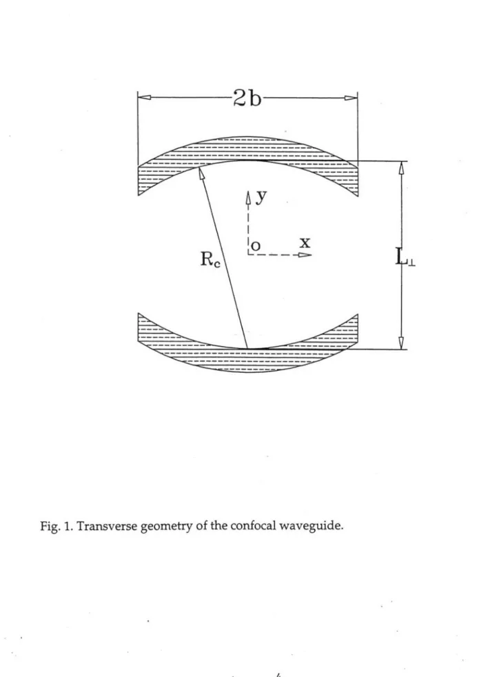
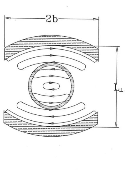
The cross section of a confocal waveguide is shown in Figure 1, and consists of two cylindrical mirrors facing each other. The distance between the two mirrors L_ is equal to the curvature radius of the mirrorR,. In other words, the geometric center of the waveguide is the focal point of the cylindrical mirrors. Such a waveguide has been utilized for RF energy transmission [9] and recently as an interaction circuit for a 100 GHz free-electron laser [10]. A section of a confocal waveguide serves as a cavity if the operating frequency is an eigenfrequency of the confocal waveguide. The eigenfrequencies and field distributions of confocal cavity modes have been calculated by previous authors [11-13]. To design the confocal cavity for a 140 GHz gyrotron, we use the quasi-optical approach and the results of numerical calculation of diffraction losses [11]. Because of diffraction at the edge of a mirror of finite width 2b, the diffraction losses are different for each cavity mode. Figure 2 plots the electric field lines in the confocal cavity mode with a Gaussian field distribution in x-direction (Fig. 1) and 6 field variations in y-direction (TEo6 mode). For the selective excitation of the Gaussian-like
mode, the mirror width has to be chosen to introduce small diffraction losses for a Gaussian-like mode, while the losses of higher-order modes with two (or more) field variations across the mirror should be much larger.
To calculate the eigenfrequencies of Gaussian-like modes, we consider the mode as the superposition of two Gaussian beams with the electric and magnetic field components
1
_1
x2 .1 kx2exp + -ky- - - -- ± i-arcta (1)
H, z w(y) 2 (y) 2 R(y) 2 kwj
where k =2r / A is a wavenumber, A is a wavelength, wo is the Gaussian beam waist size at y=O, w(y) is the Gaussian beam waist size given by:
w(y)=w + (2)
2b
A' 7-
-L0 X
'--~
-Fig. 1. Transverse geometry of the confocal waveguide.
I
---Re
2b
-- --- -_ -- - - -_ - -_ -_ - -I_ _
.. .. .. .
Fig. 2. Transverse geometry of the confocal waveguide with the annular electron beam and the electric field lines of the TE0 mode.
- - - - - - - - ---
R(y) = y I+ .2 (3)
At the mirror, where y = L / 2 , the curvature radius of the Gaussian beam's phase front
must be equal to the curvature radius of the mirror R, and therefore must satisfy
1 +(2kwo(4 R, = -Ls 1+(4) 2 LI thus, W2 L- 2 R- L L ±-L (5) 0 2k LL
The Gaussian beam spot size at the mirror is given by:
'" 0 ~ 2kW j( 2RL - L(6k
Using the boundary condition E, = 0 at the mirror, we determine the eigenvalue of the wavenumber from (1) and (5):
L
kL - arctan (7)
2RL -L2
where p is the number of field variations across L1 and is used as the mode index. The Gaussian modes supported by the confocal cavity are denoted TEOpq , where p is the transverse index, and q is the axial index. For our experiment the axial index is one. Expression (7) can be used to determine the transverse wavenumber k1 . For a confocal cavity (Rc = L1) we have from (7):
k- =P+ Ir(8) . 4 )LI
Hence, the eigenfrequency of TEopq mode is given by:
2 / 2
f = +q ,(9)
27r 4 L- L 4
where c is the speed of light and L, is the axial length of the cavity. The diffraction losses of the TEOpq mode are characterized by the
Q
factor. The transverse diffractionQ
factor due to the finite mirror width 2b isQdtf =
kL(10)
3
dif
where the losses 3df can be determined from numerical results [11] by interpolation:
log10 8di = -0.81CF +0.79 , (11)
and CF = k-b is Fresnel parameter. Expression (11) is valid if CF > 3. The axial
Q
factor of the TEopq mode is expressed as2 x 47 , q=l
Q 2 (12)
47 q
where the factor of 2 is the result of numerical simulation [4, 14]. The total diffraction
Q
factor of the cavity satisfies the following relation:1 = 1 + 1 .
(13)
~tot 1
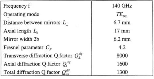
The above equations have been used to determine the confocal cavity parameters for a gyrotron oscillator experiment at 140 GHz. The results are listed in Table I.
The starting current for a gyrotron with a confocal cavity and an annular electron beam can be calculated using the linear and nonlinear theories for gyrotron oscillators with arbitrary field distributions in the cavity [4,8,15]. It is shown that the gyrotron starting current and the normalized current parameter from nonlinear theory can be expressed using the axial component of magnetic field in the gyrotron cavity:
H, (x, y, z) = I(x, y)F(z), (14)
where T(x, y) is the transverse field distribution in the cavity and F(z) is the axial field distribution. In the generalized gyrotron oscillator theory, the starting current I,, is inversely proportional to the form factor [4]
G=
I MI(rb)1
2S (15)4
|
I(x, y)J2dxdyS,
where
M, = d -+i,-- (XY) (16)
is proportional to Lorentz force at the fundamental of the cyclotron frequency, X and Y are the coordinates of the electron beam gyration centers, and S1 is a cavity cross-section area. If an annular electron beam is utilized in the gyrotron, the azimuthal average value should be taken in Eq. (15):
f +i (XY) dcp (17)
Table I
-
Design Parameters for the 140 GHz Confocal Gyrotron Experiment
Table II - Electron Beam Parameters
Frequency f 140 GHz
Operating mode TE01
Distance between mirrors L1 6.7 mm
Axial length I 17 mm
Mirror width 2b 6.2 mm
Fresnel parameter C, 4.2
Transverse diffraction
Q
factorQjf
8000 Axial diffractionQ
factorQ''
1600 Total diffractionQ factor
Q,'
1300Beam voltage 60 kV Beam current 5 A Velocity ratio a 1-1.5 Beam compression 25.5 Velocity spread 6fl /
#
5-10 % Beam radius 1.8 mm Efficiency 20 %where X = r, cos(p and Y= r, sin (p , and r, is the electron beam radius.
To derive a generalized expression for the starting current, we begin with the expression for a conventional gyrotron with a cylindrical cavity [16]:
I = 17(kA)y
#
2 ra 2 1 d , (18)2ALIIQG dpk
where
P=
,L (19)#,
A1
and P, are the transverse and axial normalized to c velocities of the electrons, y is the relativistic factor of electrons, a is the cylindrical cavity radius,0.5 2 0.5
( = JF(C)exp(iOA: )d( F2()dC (20)
-0.5 -0.5
which is a function of the transit angle
#k
= #2 pu (21)
and the relativistic gyrofrequency () B . The integrals in Eq. (20) are taken over the
normalized length = z / I, where -0.5 < < 0.5. The axial field distribution is assumed to be the Gaussian profile F(4) = exp(-4(2) for TEOpi modes, and
F( )= 2(exp(-942) for TEop
2 modes with two axial field variations. To calculate
|M1
2 in Eq. (15) for a conventional gyrotron, we use 'P(X, Y) = J. (kr)
exp(-im(p) where m isan azimuthal index (see [17]). This gives:
MI(rb )=- +± i d (X,Y)=
which leads to
|M,
(r)| = JI, (krb). The denominator in Eq. (15) can be written for aconventional gyrotron as:
x,y)|2dxdy= - 2 (ka) . (23)
Thus, the form factor for the conventional gyrotron is
jG, (kr) (24)
4J (ka) 1 72j
Equation (18) can be generalized to get an expression for the starting current of a gyrotron of arbitrary cross-section:
2f
|T(x,
y)l2dxdyI =17(kA)r /32 1 1 sd . (25)
A-1 Q
|IM
I(rb 12)y
dpk(
Note that the only change, as compared to the expression for the cylindrical gyrotron (Eq. 18), is the generalized form factor G.
A similar transformation can be used to modify the expression for the normalized current of the conventional gyrotron [18]:
I=(2
I(A) _,I 4 _A , (krb), (26)1356 1,I 4(k2a2 -m2)J(ka)
to obtain the generalized expression for arbitrary cross-section:
7 =2
/2 I(A) Qy-,/- 4 A (IM, (rb )12)A(7 1356 I 167r fI(x, y)12dxdy
We have calculated the starting current and the normalized current parameter for the confocal cavity gyrotron using Eqs. (25) and (27). Based on Eqs. (1)-(6), the axial magnetic field in the confocal cavity can be represented as follows:
T(x, y)= exp -[ 2 2 -Y k
f
(Y) (28)7w~y) 2 W2(y) 2 R(y)
where w(y) and R(y) are given by Eqs. (2) and (3) , the mode waist size is wo = , and
sin k_ y -- arctan - p = 3,5,7,...
f
(y)= LI (29)cos k y - arctan p = 4,6,8,...
2 L±)I
The derivatives -- and - were derived from Eqs. (28) and (29) analytically, and
dx dy
substituted into Eq. (17) to calculate (IM12 numerically. We also derived from Eqs.
(28) and (29) the integral over the confocal cavity cross-section:
I'(x, y)|2dxdy = Lf 2()dy . (30)
s 2kL
As a result, the confocal cavity gyrotron starting current can be written as follows:
L
J2f2(y)dyI, =17(kA)y
#12
2k d k (31)Qec
(rf
dby(2 )5/2 1 14 A IM
)A2
7 1356(A) L,1 f
8 -J- 2f2(y)dy 2kmLI
Based on the cavity design in Table I, some theoretical features of the confocal gyrotron oscillator have been numerically calculated for an electron beam voltage of 80 kV, velocity ratio a =
#_1
/fi, =1, normalized length of 8.87, and beam radius r, of 1.8 mm. Based on these parameters, the value ofI
M I ) is 0.276. Assuming the external magnetic field is set at the nominal operating point of 5.6 T, the transit angle ok given byEq. (21) is 4.46, the function P(#k)is 0.227, the derivative d0 / dois -0.164, and the confocal gyrotron starting current I, ~ 2A .
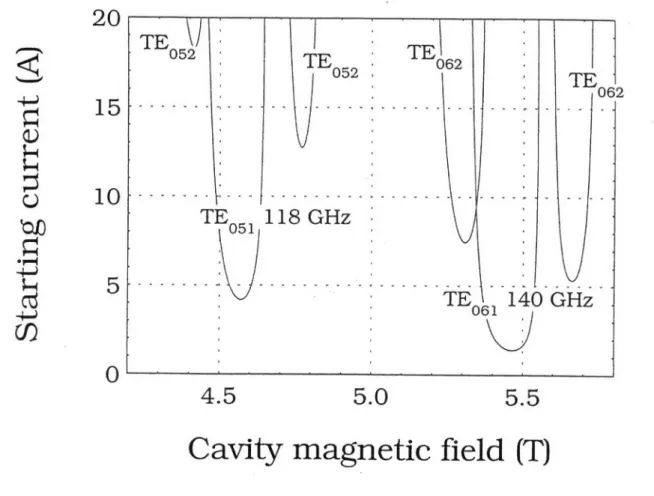
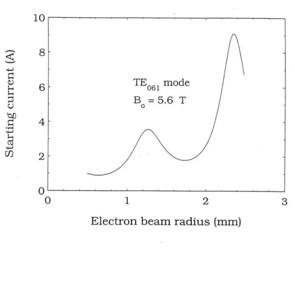
The dependence of starting current of the confocal gyrotron on the cavity magnetic field B is plotted in Fig. 3 for the TE0 6 1 mode at 140 GHz and for the TE0 51 mode at 118 GHz, as well as for the higher order spurious modes TE062 and TE0 52. One can see that the
minimum starting current of spurious oscillations is well above the operating current of 5 A. Thus, confocal gyrotron starting current calculations predict that only the TE05 1 and TE0 61 modes separated by a 22 GHz interval will be excited. The starting current as a function of the beam radius for the TE0 6 1 mode at 140 GHz and a cavity magnetic field B=5.6 T is plotted in Fig. 4. This graph indicates that the beam radius of 1.8 mm corresponds to a local minimum of the starting current, or alternatively, to strong coupling between the beam and RF field.
For a 5 A beam current, the normalized current parameter (32) is calculated to be 7 =0.045. From nonlinear gyrotron analysis [18] we can find that the transverse efficiency 77_ corresponding to this current parameter is 60%, and the total efficiency 7 =
7
1a 2 /(1 + a 2)=41% for a velocity ratio a of 1.5. The starting current calculation(linear theory), and the efficiency estimation using nonlinear theory, thus demonstrate the possibility of high power operation in the confocal gyrotron at 140 GHz. However, because the coupling between the beam and standing RF field varies azimuthally in the confocal gyrotron, the anticipated efficiency will not be as large as in the cylindrical cavity gyrotron with its pure rotating mode. This effect can be minimized by proper selection of the beam radius. We also expect the efficiency to be lowered by the beam
062
TE
062
T
06140GHz
5.5
Cavity magnetic field (T)
Fig. 3. Confocal gyrotron starting current as a function of magnetic field.
20
TE 0 5 2 ,s ITE
15
10
5
YI)
TEo
TE
0111 - .. . -. .4.5
8 GHz
5.0
0
10i
6
4
4-U)2
0
0
1
2
3
Electron beam radius (mm)
Fig. 4. Confocal gyrotron starting current as a function of the beam radius for the
TE., mode.
TE
061modeB = 5.6 T
velocity spread. Taking all these factors into account, we expect the efficiency for the 140 GHz experiment to be between 20-25%.
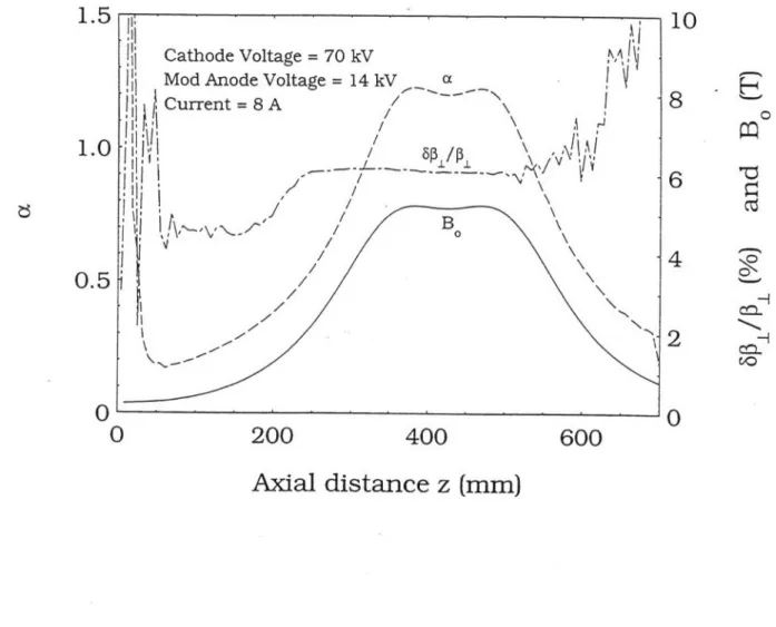
The confocal gyrotron was designed to be experimentally studied using a magnetron-injection gun (MIG) designed for 140 GHz operation in a 6 T superconducting magnet. The electron beam code EGUN [19] was employed to analyze the annular beam produced by the MIG and simulate the propagation of the beam in the confocal gyrotron. The results of the EGUN simulation are presented in Fig. 5. The simulation predicts good beam quality at the cavity, which is located at an axial distance of 45 cm, with a perpendicular velocity spread of 6% and a velocity ratio of 1.3. The beam parameters used in the design of the 140 GHz TE06 1 mode confocal gyrotron experiment are listed in Table II.
III. Experimental Results
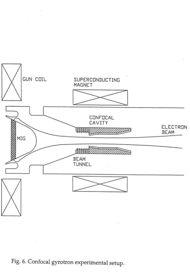
A schematic of the gyrotron experiment is shown in Fig. 6. The electron beam formed by the triode MIG propagates through the beam tunnel to the confocal cavity. The MIG was designed to be used with the combined field of the main superconducting magnet, and a room temperature gun coil capable of 0.2 T magnetic fields. The cavity is made of three sections: a 5 degree down taper, a straight confocal waveguide section, and a 5 degree up taper. The microwaves generated in the cavity are radiated into a cylindrical pipe that serves as the collector and the output waveguide. The microwaves are transmitted by this pipe to a quartz vacuum window and radiated into free space. The 140 GHz confocal gyrotron design was based on a 6 T superconducting magnet available at MIT, and optimized for the field profile of that magnet. The experimental data presented here was obtained using both this magnet, and a 9 T magnet with a different profile. We anticipated that the power generated by the gyrotron in the latter experiments would be lower because the field profile of the 9 T magnet was not optimum. This was confirmed experimentally. However, the data using the 9 T magnet is useful because it does demonstrate the effectiveness of the confocal cavity in controlling modes.
The high voltage for the MIG is provided by a modulator capable of producing up to 150 kV, 3 gs pulses. The high voltage is measured using a capacitance voltage divider. The beam current is measured using a Rogowski coil. The modulator can run at repetition rates of up to 4 Hz. The RF output signal is measured with a RF diode with a horn as a receiver. All the measured signals are transmitted to digital scopes. A typical set of
Cathode Vol Mod.Anode Current = 8. t I age = 70 kV
M
\ oltage = 14 kV a //~ 8f /[ .\b
1 L J r/IN'
0200
400
600
10
8
06
42
0
Axial distance z (mm)
Fig. 5. EGUN simulated electron beam quality for the confocal gyrotron.
1.5
1.0
0.5
0
1GUN COIL SUPERCONDUCTING MAGNET
Fig. 6. Confocal gyrotron experimental setup.
CAVIT EET RO MIG BEAM /F//// TUNNEL N
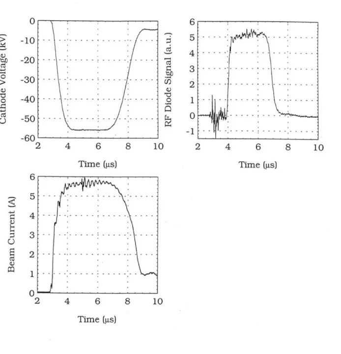
measured data is shown in Fig. 7, with traces of the RF pulse with a width of 2.6 Ps, beam voltage (63 kV) and beam current (5.4 A). The diode noise at 3 Rs in Fig. 7 is due to the thyratron switch of the power supply. The frequency of the gyrotron RF output was measured with a harmonic mixer and a digital scope which can perform a FFT. A 0.3 GHz intermediate frequency is utilized in this mixer. The accuracy of frequency measurement is ±10 MHz , and allows us to accurately identify the gyrotron modes. The average output RF power is measured using a 4 inch diameter calorimeter placed about 1 inch from the output window. Using the diode trace for the pulse width, the peak power of the gyrotron can be determined taking into account the 2 Hz repetition rate and the calorimeter absorption of 0.85 .
The first step of the gyrotron operation is the alignment of the beam axis with the cavity axis. The alignment is critical for the coupling between the electron beam and the cavity mode. Precision alignment is achieved by monitoring beam interception by a metal ring (beam scraper) located in the beam tunnel. The beam scraper is positioned right before the cavity with an aperture radius of 2.5 mm. During the alignment, the tube is translated horizontally and vertically until the beam scraper starts to intercept the beam. These locations are recorded by two micrometers, and the central position is the aligned position for the tube. To excite and optimize a particular gyrotron mode, one can adjust the cathode voltage, mod-anode voltage, beam current, cavity magnetic field using the superconducting solenoid and cathode magnetic field using the gun coil. By sweeping the magnetic field and fine tuning other parameters, the strong cavity modes were excited and used to optimize the coupling.
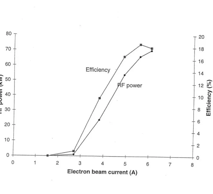
A maximum efficiency of 18.5% with RF power of 66 kW was generated by the confocal gyrotron when operating in the 135.98 GHz TE061 mode during experiments using the 6 T magnet. This result was obtained using a magnetic field of 5.36 T, a beam voltage of 62.5 kV and a current of 5.6 A. Figure 8 shows the efficiency and RF output power as a function of beam current at constant voltage of 60 kV, and constant velocity ratio of about 1.2. The output power curve starts at a minimum current of 2.7 A and scales almost linearly with the current, while the efficiency increases to a maximum and then saturates. Although the curve shows no measurable power below the current of 2.7 A, the mode is weakly present at currents as low as 1.5 A based on heterodyne interferometry measurements. The reason that this mode has such low starting current can be explained by the beam velocity spread, which is estimated to be around 7% by EGUN simulations
- - - -. . -
----
- ---- --.. .. ...
.--10 -20 -30 -40 -50 C o -60' 2 4 6 8 10 Time (gs) 5 4 3 2 1 0 -1 2 4 6 8 10 Time (gs) 6 5 4 3 2 1 0 2 4 6 8 10 Time (gs)Fig. 7. Typical signal traces measured from the 140 GHz confocal gyrotron experiment. o0 0 -4-j H C-)
S
- -- -- - - --- --- - --- - - - - -- -- --- -- - - - ---
-6 080 20 70 18 60 16 Efficiency 14 50 F power 12 40 ----1 10 -30 8 20- 6 4 10 2 0- 0 0 1 2 3 4 5 6 7 8
Electron beam current (A)
Fig. 8. RF output power and efficiency measured as a function of the beam current.
factors. So, even at low current, a portion of the beam with high velocity can still excite the mode without substantial power.
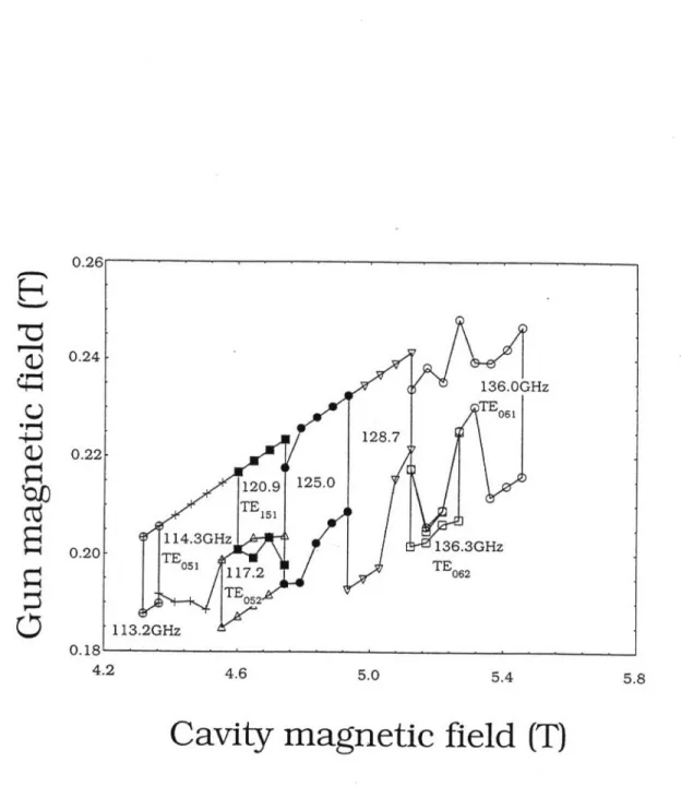
A mode map was constructed for all the modes that could be excited in the confocal gyrotron. By sweeping both the cavity and cathode magnetic fields, we observed gyrotron emission in different modes with different frequencies. Sweeping the cavity magnetic field allowed us to change the electron cyclotron frequency, and thus the mode frequency, while sweeping the cathode magnetic field enabled us to change the electron beam radius in the cavity and therefore achieve coupling with all possible modes. Figure 9 shows a measured mode map using the 9 T magnet. This mode map plots regions of single mode emission. The lower right comer of Fig. 9 corresponds to high beam compression and, as a result, electron beam reflection occurs. The upper left region is the low magnetic compression region where the beam radius becomes too large and can be intercepted by the beam scraper. The strongest modes observed were the TE051 and TE0 61 modes at the expected cavity magnetic fields.
Figure 10 shows the RF power versus the cavity magnetic field for the modes observed in Fig. 9. The mode map is dominated by the two modes at 114.33 GHz and 135.98 GHz with substantial output RF power. Ignoring a small correction in the confocal cavity frequency due to I, in Eq. (9) , we get the theoretical ratio of the TE061 and TE05 1 mode frequencies 6.25/5.25=1.19, which agrees with the experimentally observed ratio of 1.189. This is convincing evidence that these two dominant modes are the two confocal cavity modes TE061 and TE051. The other modes observed and shown on the mode map (Fig. 9) were generated with low output power. The mode corresponding to 136.3 GHz is probably the TE062, while 120.9 GHz. matches well with the TE151 mode. The other observed frequencies at very low power could not be matched with cavity modes, but may be associated with oscillations in other parts of the tube, such as in the beam tunnel.
IV. Conclusions
We have successfully conducted a confocal gyrotron oscillator experiment at 140 GHz. This is the first experimental demonstration of a mode-selective gyrotron with an open confocal cavity. The oscillator's cavity design was based on a moderately overmoded confocal cavity with open sides to eliminate competing modes. The modeling of the confocal structure was adapted from Weinstein's theory [11]. For the TE0 61 operating mode, the confocal cavity's width was set at 6.2 mm, and the distance between the
120.9 TE 1 51 114.3GHz TE0 51 117.2 TEs2A 113.2GHz 4.2 125.0 4.6 128.7 5.0 136.0GHz TE0 6 1 06 136.3GHz TE0 6 2 5.4 .
Cavity magnetic field (T)
Fig. 9. Map of observed modes as a function of the gun and cavity magnetic fields. 2G6. 0.24
I-H
0 Q 0S
0
0.22 0.20 0. 5.4 5.8*I.
I
4.4 4.6 4.8 5 5.2
Cavity magnetic field (T)
5.4 5.6 5.8
Fig. 10. Optimized RF output power from the different modes as a function of cavity magnetic field.
35 30-- 25-- 20-0 cL
15
10 5-+ 0 4.2cavity's mirrors was chosen to be 6.7 mm. By varying the cavity width, we controlled the amount of cavity diffraction losses for different modes, and thus increased the starting currents of competing modes. This was the primary mechanism of mode selectivity in the confocal gyrotron. The design resulted in a 22 GHz frequency difference between the desired TE061 mode at 136 GHz, and the nearest competing mode (TE051) at 114 GHz. Although other modes were observed experimentally, they were weak and could likely be eliminated with further refinement of the cavity design.
The confocal gyrotron generated up to 66 kW of RF power at 136.0 GHz with an efficiency of 18%. The confocal cavity's sparse mode spectrum was demonstrated by this experiment. The paucity of modes observed with this structure has significant implications in the development of high frequency, high power gyro-TWT amplifiers, where mode purity is a critical issue. The use of a confocal waveguide would allow stable operation in high order modes, which are required for high power amplifier operation. In addition to effectively controlling the mode spectrum, the confocal waveguide would also be ideal for a gyro-TWT because it would allow efficient quasi-optical injection and extraction of the RF beam.
Acknowledgments
The authors are grateful to Dr. T.Kimura for his help during this experiment. The authors thank Dr. G.S.Nusinovich for very helpful discussions.
References
1. K.E.Kreischer, J.B.Schutkeker, B.G.Danly, W.J.Mulligan, and R.J.Temkin, "High efficiency operation of a 140 GHz pulsed gyrotron," Int. J. Electronics, vol. 57, no. 6, pp. 835-850, 1984.
2. K.Felch, M.Blank, P.Borchard, T.S.Chu, J.Feinstein, H.R.Jory, J.A.Lorbeck, C.M.Loring, Y.M.Mizuhara, J.M.Neilson, R.Schumacher, and R.J.Temkin, "Long-pulse and CW tests of a 1 10-GHz gyrotron with an internal, quasi-optical converter," IEEE Trans. Plasma Sci., vol. 24, no. 3, pp. 558-569, 1996.
3. K.E.Kreischer, T.Kimura, B.G.Danly, and R.J.Temkin, "High-power operation of a 170 GHz megawatt gyrotron," Phys. Plasmas, vol. 4, no. 5, pp. 1907-1914, 1997.
4. A.V.Gaponov, V.A.Flyagin, A.L.Goldenberg, G.S.Nusinovich, Sh.E.Tsimring, V.G.Usov, and S.N.Vlasov, "Powerful millimeter-wave gyrotrons," Int. J. Electronics, vol. 51, no. 4, pp. 277-302, 1981.
5. A.W.Fliflet, T.A.Hargreaves, W.M.Manheimer, R.P.Fisher, M.L.Barsanti, B.Levush, and T.Andersen, "Operating characteristics of a continuous-wave-relevant quasioptical gyrotron with variable mirror separation," Phys. Fluids B, vol. 2, no. 5, pp. 1046-1056, 1990.
6. S.Alberti, M.Q.Tran, J.P.Hogge, T.M.Tran, A.Bondeson, P.Muggli, A.Perrenoud, B.Jodicke, and H.G.Mathews, "Experimental measurements on a 100 GHz frequency tunable quasioptical gyrotron," Phys. Fluids B, vol. 2, no. 7, pp. 1654-1661, 1990.
7. I.I.Antakov, S.N.Vlasov, V.A.Gintsburg, L.I.Zagryadskaya, and L.V.Nikolaev, "CRM generators with mechanical frequency detuning," Elektron. Tekh., ser. 1: Elektronika SVCh, no. 8, pp. 20-25, 1975 (in Russian).
8. A.G.Luchinin and G.S.Nusinovich, "An analytical theory for comparing the efficiency of gyrotrons with various electrodynamic systems," Int. J. Electronics, vol. 57, no. 6, pp. 827-834, 1984.
9. T.Nakahara and N.Kurauchi, "Guided beam waves between parallel concave reflectors," IEEE Trans. Microwave Theory Tech., vol. 15, no. 2, pp. 66-71, 1967.
10. I.M.Yakover, Y.Pinhasi, and A.Gover, "Resonator design and characterization for the Israeli tandem electrostatic FEL project," Nucl. Instrum. Methods Phys. Res., vol. A358, pp. 323-326, 1995.
11. L.A.Weinstein, Open Resonators and Open Waveguides. Boulder: Golem Press, 1969.
12. N.N.Voitovich, B.Z.Katsenelenbaum, and A.N.Sivov, "The generalized natural-oscillation method in diffraction theory," Sov. Phys. Uspekhi, vol. 19, no. 4, pp. 337-352, 1976.
13. V.P.Shestopalov and Y.V.Shestopalov, Spectral Theory and Excitation of Open Structures. London: IEE, 1996.
14. S.N.Vlasov, G.M.Zhislin, I.M.Orlova, M.I.Petelin, and G.G.Rogacheva, "Irregular waveguides as open resonators," Radiophys. Quantum Electron., vol. 12, pp. 972-978, 1969.
15. M.I.Petelin, "Self-excitation of oscillations in a gyrotron," Gyrotrons. Gorky: Inst. Appl. Phys., 1981, pp. 5-25 (in Russian).
16. V.L.Bratman, N.S.Ginzburg, G.S.Nusinovich, M.I.Petelin, and P.S.Strelkov, "Relativistic gyrotron and cyclotron autoresonance masers," Int. J. Electronics, vol. 51, no. 4, pp. 541-567, 1981
17. G.S.Nusinovich and H.Li, "Theory of gyro-traveling-wave tubes at cycloton harmonics," Int. J. Electronics, vol. 72, no. 5 and 6, pp. 895-907, 1992.
18. B.G.Danly, and R.J.Temkin, "Generalized nonlinear harmonic gyrotron theory," Phys. Fluids, vol. 29, no. 2, pp. 561-567, 1986.