HAL Id: hal-00329215
https://hal.archives-ouvertes.fr/hal-00329215
Submitted on 1 Jan 2001
HAL is a multi-disciplinary open access
archive for the deposit and dissemination of
sci-entific research documents, whether they are
pub-lished or not. The documents may come from
teaching and research institutions in France or
abroad, or from public or private research centers.
L’archive ouverte pluridisciplinaire HAL, est
destinée au dépôt et à la diffusion de documents
scientifiques de niveau recherche, publiés ou non,
émanant des établissements d’enseignement et de
recherche français ou étrangers, des laboratoires
publics ou privés.
Coordinated Cluster, ground-based instrumentation and
low-altitude satellite observations of transient
poleward-moving events in the ionosphere and in the tail
lobe
M. Lockwood, H. Opgenoorth, A. P. van Eyken, A. Fazakerley, J.-M.
Bosqued, W. Denig, J. A. Wild, C. Cully, R. Greenwald, G. Lu, et al.
To cite this version:
M. Lockwood, H. Opgenoorth, A. P. van Eyken, A. Fazakerley, J.-M. Bosqued, et al.. Coordinated
Cluster, ground-based instrumentation and low-altitude satellite observations of transient
poleward-moving events in the ionosphere and in the tail lobe. Annales Geophysicae, European Geosciences
Union, 2001, 19 (10/12), pp.1589-1612. �hal-00329215�
Annales Geophysicae (2001) 19: 1589–1612 c European Geophysical Society 2001
Annales
Geophysicae
Coordinated Cluster, ground-based instrumentation and
low-altitude satellite observations of transient poleward-moving
events in the ionosphere and in the tail lobe
M. Lockwood1, 2, H. Opgenoorth3, A. P. van Eyken4, A. Fazakerley5, J.-M. Bosqued6, W. Denig7, J. A. Wild8, C. Cully9, 3, R. Greenwald10, G. Lu11, O. Amm12, H. Frey21, A. Strømme13, P. Prikryl14, M. A. Hapgood1, M. N. Wild1, R. Stamper1, M. Taylor5, I. McCrea1, K. Kauristie12, T. Pulkkinen12, F. Pitout3, A. Balogh15, M. Dunlop15, H. R`eme6, R. Behlke3, T. Hansen13, G. Provan8, P. Eglitis3, S. K. Morley2, D. Alcayd´e6, P.-L. Blelly6, J. Moen16, 17, E. Donovan9, M. Engebretson18, M. Lester8, J. Watermann19, and M. F. Marcucci20
1Solar Terrestrial Physics Division, Space Science and Technology Department, Rutherford Appleton Laboratory, Chilton,
Didcot, Oxfordshire, UK
2Department of Physics and Astronomy, Southampton University, Southampton, UK 3IRF, Swedish Institute of Space Physics, Uppsala Division, Sweden
4EISCAT Scientific Association, Longyearbyen, Svalbard, Norway 5Mullard Space Science Laboratory, Holmbury St. Mary, Surrey, UK 6CESR, Centre d’Etude Spatiale des Rayonnements, Toulouse, France
7Space Vehicles Directorate, Air Force Research Laboratory, Hanscom AFB, Massachusetts, USA 8Department of Physics and Astronomy, Leicester University, Leicester, UK
9University of Calgary, Calgary, Canada
10Remote Sensing Group, Applied Physics Laboratory, John Hopkins University, Laurel, MD, USA 11High Altitude Observatory, National Center for Atmospheric Research, Boulder, Colorado, USA 12Finnish Meteorological Institute, Helsinki, Finland
13University of Tromsø, Tromsø, Norway
14Communications Research Centre, Ottawa, Ontario, Canada 15Blackett Laboratory, Imperial College, London, UK
16Department of Physics, University of Oslo, Blindern, Oslo, Norway
17Also at Arctic Geophysics, University Courses on Svalbard, Longyearbyen, Norway 18Department of Physics, Augsburg College, Minneapolis, MN, USA
19Danish Meteorological Institute, Copenhagen, Denmark
20Istituto di Fisica dello Spazio Interplanetario - CNR, Rome, Italy 21University of California, Berkeley, California, USA
Received: 18 April 2001 – Revised: 19 May 2001 – Accepted: 18 July 2001
Abstract. During the interval between 8:00–9:30 on 14 Jan-uary 2001, the four Cluster spacecraft were moving from the central magnetospheric lobe, through the dusk sector man-tle, on their way towards intersecting the magnetopause near 15:00 MLT and 15:00 UT. Throughout this interval, the EIS-CAT Svalbard Radar (ESR) at Longyearbyen observed a se-ries of poleward-moving transient events of enhanced F-re-gion plasma concentration (“polar cap patches”), with a rep-etition period of the order of 10 min. Allowing for the es-timated solar wind propagation delay of 75 (±5) min, the interplanetary magnetic field (IMF) had a southward com-ponent during most of the interval. The magnetic footprint of the Cluster spacecraft, mapped to the ionosphere using the Tsyganenko T96 model (with input conditions prevail-ing durprevail-ing this event), was to the east of the ESR beams.
Correspondence to: M. Lockwood ([email protected])
Around 09:05 UT, the DMSP-F12 satellite flew over the ESR and showed a sawtooth cusp ion dispersion signature that also extended into the electrons on the equatorward edge of the cusp, revealing a pulsed magnetopause reconnection. The consequent enhanced ionospheric flow events were im-aged by the SuperDARN HF backscatter radars. The aver-age convection patterns (derived using the AMIE technique on data from the magnetometers, the EISCAT and Super-DARN radars, and the DMSP satellites) show that the asso-ciated poleward-moving events also convected over the pre-dicted footprint of the Cluster spacecraft. Cluster observed enhancements in the fluxes of both electrons and ions. These events were found to be essentially identical at all four space-craft, indicating that they had a much larger spatial scale than the satellite separation of the order of 600 km. Some of the events show a correspondence between the lowest energy
1590 M. Lockwood et al.: Coordinated observations of transient poleward-moving events magnetosheath electrons detected by the PEACE instrument
on Cluster (10–20 eV) and the topside ionospheric enhance-ments seen by the ESR (at 400–700 km). We suggest that a potential barrier at the magnetopause, which prevents the lowest energy electrons from entering the magnetosphere, is reduced when and where the boundary-normal magnetic field is enhanced and that the observed polar cap patches are pro-duced by the consequent enhanced precipitation of the lowest energy electrons, making them and the low energy electron precipitation fossil remnants of the magnetopause reconnec-tion rate pulses.
Key words. Magnetospheric physics (polar cap phenomena; solar wind – magnetosphere interactions; magnetosphere – ionosphere interactions)
1 Introduction
1.1 Poleward-moving transient events in the cusp/cleft The cusp/cleft aurora, dominated by 630 nm red line emis-sions from atomic oxygen, shows a series of poleward-moving events when the interplanetary magnetic field (IMF) points southward (e.g. Sandholt et al., 1992; Fasel, 1995). Using the European Incoherent Scatter (EISCAT) UHF and VHF incoherent scatter radars, these cusp/cleft auro-ral transients have been shown to be associated with tran-sient flow bursts (Lockwood et al., 1989a, b; 1993a, b; Moen et al., 1995; 1996a) and consequent ion-neutral heating of the ionospheric ion gas (Lockwood et al., 1993a, b; 1995a). These events are quasi-periodic with a distribution of re-peat intervals between about 1 and 30 min, giving a mean value of about 7 min, but a mode value of about 3 min (Fasel, 1995). This distribution is very similar to that of “flux trans-fer events” (FTEs) on the dayside magnetopause (Lockwood and Wild, 1993). However, in both cases, the low-period part of the distribution is likely to be set by instrument sensitivity and the criterion used to define events (as demonstrated by a comparison of the results of Kuo et al. (1995) with those by Lockwood and Wild). The transient auroral events are seen to form within the LLBL (cleft) precipitation, near the equa-torward edge of the cusp/cleft aurora (Moen et al., 1996b) and subsequently migrate poleward into the regions of the cusp and then the mantle precipitations, which is consistent with the evolution of newly-opened field lines (Lockwood et al., 1989a, b; Cowley et al., 1991b; Sandholt et al., 1992; Lockwood et al., 1993a, c). The transient auroral events in the northern hemisphere also move westward/eastward when the IMF by component is positive/negative (e.g. Lockwood et al., 1993a; Milan et al., 2000), as predicted for the curva-ture (“tension”) force on the newly-opened field lines. The repetitive pattern of formation and motion of these events shows that the patches of field lines are produced by pulses in the reconnection rate (Lockwood et al., 1995a) and not by steady reconnection in the presence of oscillations in the Y component of the magnetic field in interplanetary space
(Stauning, 1994; Stauning et al., 1994, 1995) or in the mag-netosheath (Newell and Sibeck, 1993). This pattern of event motion is also consistent with the asymmetric MLT distribu-tions of their occurrence for BY >0 and BY <0 (Karlson et al., 1996), as discussed by Cowley et al. (1991a).
Pinnock et al. (1993) used HF coherent scatter radars to image these transient flow channels in the cusp/cleft region and Milan et al. (1999) have shown that they are indeed asso-ciated with the poleward-moving 630 nm optical transients. In addition, Milan et al. (2000) have shown that the flow channels are also associated with poleward-moving forms seen in global images of the UV aurora. These UV aurora, such as the 557.7 nm (atomic oxygen green line) aurora stud-ied by Lockwood et al. (1993a), are coincident with the sheet of upward field-aligned current of the opposite directed pair that is required to transfer the motion of the newly-opened flux into the ionosphere. Lockwood et al. (2001b) have pre-dicted that these arcs will form at the shear in the longitudinal flow speeds at the boundaries between events. The east-west direction of the flow in the channels seen by HF radars is controlled by the prevailing IMF BY(Provan et al., 1998) and their motion, as for the optical transients, is consistent with their occurrence as a function of local time (Provan and Yeo-man, 1999; Provan et al., 1999). McWilliams et al. (2000) have shown that the distribution of repeat periods of these enhanced flow events is very similar to the corresponding distributions for 630 nm cusp/cleft auroral transients, as re-ported by Fasel et al., and for magnetopause FTE events, as reported by Lockwood and Wild. From the ground-based op-tical observations, global UV images and radar observations, events are found to be typically 100–300 km in latitudinal width and to vary in longitudinal extent up to about 2000 km (Lockwood et al., 1990; 1993a; Pinnock et al., 1995; Milan et al., 2000). Such dimensions and the repetition rates mean that these events are major, and sometimes the dominant drivers of convection (Lockwood et al., 1993a; 1995b; Milan et al., 2000).
1.2 Cusp ion steps
Another predicted signature of pulsed reconnection are discontinuities in the dispersion of injected solar wind ions in the cusp region, called “cusp ion steps” (Cow-ley et al., 1991b; Lockwood and Smith, 1992, 1994; Escou-bet et al., 1992; Lockwood and Davis, 1996). These were first reported in low-altitude satellite data by Newell and Meng (1991). An important part of the prediction of these events was the model of ionospheric flow excitation by Cow-ley and Lockwood (1992) which predicts that patches of newly-opened flux would be appended directly adjacent to each other. Periods of low or zero reconnection rate be-tween pulses give discontinuous steps in the ion dispersion characteristics at the boundaries between these patches: this is due to the discontinuous change in time elapsed since the field line was reconnected. Modelling of the effects of pulsed magnetopause reconnection has been shown to re-produce the observed simultaneous steps in both downward
M. Lockwood et al.: Coordinated observations of transient poleward-moving events 1591 moving and upward moving ions in the cusp at middle
al-titudes, unambiguously demonstrating that these events are caused by pulsed reconnection and not by pulsed plasma transfer across the magnetopause (Lockwood et al., 1998). Cusp ion steps have been seen in association with poleward-moving patches of elevated electron temperature (detected by incoherent scatter radar) by Lockwood et al. (1993b), with poleward-moving cusp/cleft auroral transients by Far-rugia et al. (1998) and with poleward-moving flow chan-nel events by Yeoman et al. (1997). Pinnock et al. (1995) found some poleward-moving flow channels (detected by HF radar) were in association with a seemingly different “saw-tooth” signature in the cusp ions. However, modelling by Lockwood and Davis (1996) showed that this sawtooth sig-nature was, in fact, the same phenomenon as the cusp ion steps seen by Lockwood et al. (1993b), with the differences arising purely from the longitudinal, as opposed to the more meridional nature of the satellite pass. Recently, Morley and Lockwood (2001) have pointed out that for a general satel-lite orbit orientation, the form of the dispersion also depends on the amplitude of the reconnection rate pulses: sawtooth signatures will become stepped signatures as the amplitude increases.
1.3 Polar cap patches
The enhanced 630 nm emission in poleward-moving cusp/cleft transients is caused by the hot tail of a heated thermal electron population (Wickwar and Kofman, 1984; Lockwood et al., 1993a). The magnetosheath electron precipitation is responsible for that heating, but not for the direct excitation of the emission. Emission intensity is also enhanced by higher ionospheric plasma concentration, and this too can result in more particles in the hot tail of the distribution with sufficient energy to cause excitation of the 630 nm emission. Patches of enhanced plasma concentration convecting anti-sunward are a common feature of the polar cap during southward IMF (Weber et al., 1984; Sojka et al., 1993, 1994, McEwen and Harris, 1996). These are seen convecting through the cusp/cleft region and into the polar cap (Foster and Doupnik, 1984; Foster, 1989; Lockwood and Carlson, 1992; Valladares et al., 1994; Prikryl et al., 1999a, b) and thus, it is likely that they are the fossil remnants of the poleward-moving cusp/cleft transient events.
1.4 The minima separating transient events
One major unresolved question about both poleward-moving 630 nm cusp/cleft transients and polar cap patches is why minima (in luminosity and plasma concentration, respec-tively) are seen between them. The successful theory of the cusp ion precipitation is based on the concept that each newly-opened field line evolves in a similar manner, such that the ion characteristics depend only on the time elapsed since reconnection. Although pulsed reconnection gives the dis-continuities in their energy dispersion within the cusp/cleft region, magnetosheath ions are found in a single contiguous
region of newly-opened field lines and one would expect this to also be true of the injected magnetosheath electron pop-ulation. Thus, on its own, this model does not explain the minima between events and an additional mechanism must be invoked (Davis and Lockwood, 1996). A variety of candi-date mechanisms have been proposed.
Lockwood and Carlson (1992) interpreted the concentra-tion variaconcentra-tions, using the model of ionospheric convecconcentra-tion excitation by Cowley and Lockwood (1992) (which led to the prediction of cusp ion steps), as the result of changes in the pattern of flow modulating the entry into the polar cap of the EUV-produced sub-auroral plasma. However, Rodger et al. (1994a, c) pointed out that plasma produc-tion by soft particle precipitaproduc-tion (Whitteker, 1977; Water-mann et al., 1992; Davis and Lockwood, 1996; Millward et al., 1999) and plasma loss by enhanced electric fields and re-action rates (Schunk et al., 1975; Jenkins, 1997; Balmforth et al., 1998, 1999) must also be significant factors in intro-ducing structure into the plasma concentrations on the time scales for flux tubes to enter the polar cap. In time-varying cases, it may be possible for some flux tubes entering the po-lar cap to have undergone one or both of these processes to a greater degree than others. Lockwood et al. (2000) argued that variation may also be brought about by local time vari-ations in the injected magnetosheath electron population and in the tension force on the newly-opened field lines, provided that the events are sufficiently extensive in longitude. An-other possibility, modelled by Davis and Lockwood (1996), is that the electron precipitation spectrum hardens in regions of upward field-aligned currents, such that the underlying E-region is enhanced rather than the F-region. Lockwood et al. (1993a; 2001b) have presented evidence that this does occur in the expected locations since both green line and UV auroral transients on the relevant edge of the patches on newly-opened flux can be identified.
The present paper considers another potential explanation that has not been considered previously. It presents the first observations of ionospheric polar cap patches that can be associated with electron flux variations in the high-altitude mantle region, i.e. near the sunward edge of the tail lobe at a geocentric distance of around 10 RE(a mean Earth radius, 1 RE =6370 km). These data strongly imply that some of the patches are produced by modulations in the lowest energy of magnetosheath electrons, caused either by a potential bar-rier of varying amplitude at the magnetopause or by fluctua-tions in the electron spectrum present in the magnetosheath before the reconnection occurred. The IMF in the interval studied was predominantly southward (Sect. 2.1). The iono-spheric measurements of patches are made by the EISCAT Svalbard radar (ESR), which tracked the patches as they mi-grated poleward into the polar cap (Sect. 2.3). The lobe measurements were made by the four Cluster-2 spacecraft (Sect. 2.6). Low-altitude satellite data reveal cusp ion steps (Sect. 2.2). Data from the SuperDARN HF coherent radars and magnetometers also reveal fluctuations in the character-istic repeat period of the order of 10 min (Sect. 2.5). There-fore, we discuss all the data (from Cluster, from the
ground-1592 M. Lockwood et al.: Coordinated observations of transient poleward-moving events ESR poleward beam DMSP-F12 orbit cusp auroral oval Cluster ESR field-aligned beam 0 kV +10 kV -10 kV +20 kV +30 kV +40 kV AMIE equipotentials IMAGE, FUV Imager / WIC 09:05 UT 14 January 2001 transpolar voltage = 54 kV 12 06 18 MLT = 0 hrs ΛΛΛΛ = 50°°°°
Fig. 1. The locations of the coordinated measurements on 14 January 2001 in an invariant latitude (3), with magnetic local time (MLT)
frame at 09:05 (the time of the closest approach of the DMSP-F12 satellite to the ESR field-aligned beam). The footprint of the centroid of the Cluster tetrahedron is mapped down to the northern hemisphere ionosphere using the Tsyganenko T96 model with average input parameters for the interval studied here (see text for details). The plot also shows in white the locations of the two beams employed by the EISCAT Svalbard Radar (ESR) on this day. The pass of the DMSP-F12 satellite at 08:54–09:12 UT is shown, with thicker segments denoting where the satellite intersected the dusk auroral oval and the cusp. The orange contours are convection equipotentials, derived by the AMIE technique employing magnetometer, SuperDARN, DMSP and ESR observations. These are superposed on observations of auroral emissions made at this time by the WIC of the FUV imager on the IMAGE satellite.
based instruments and from low-altitude spacecraft) in terms of the effects of pulsed magnetopause reconnection (Sect. 3).
2 Observations
2.1 Overview and interplanetary conditions
On 14 January 2001, the four Cluster spacecraft approached the magnetopause from the tail lobe, following a path close to the 15:00 MLT meridian. Simultaneous measurements were made using a wide array of ground-based instrumentation. An overview of this pass and of the instrumentation deployed is given by Opgenoorth et al. (2001, this issue). Figure 1 is an invariant latitude (3) – magnetic local time (MLT) plot of the locations of the various observations at 09:05 on this day. The plot also shows the flow equipotentials and the location of Far Ultraviolet (FUV) auroral emissions at this time (see Sects. 2.5 and 2.6, respectively). The magnetic footprint of the Cluster spacecraft was mapped to the ionosphere using the Tsyganenko T96 model with input conditions observed by ACE at 07:50 UT (IMF BX = −3 nT, BY = +2 nT,
BZ = −3 nT, solar wind concentration Nsw = 2.0 cm−3 and velocity Vsw =400 km s−1, giving a dynamic pressure Psw =0.6 nPa) and with the geomagnetic index of Dst = 0. These input conditions are based on a derived propagation delay from ACE to the magnetosphere of 75 min (see below). Also shown in Fig. 1 are the two beams of the ESR (Mc-Crea and Lockwood, 1997), deployed pointing along the ge-omagnetic field line from Longyearbyen and with a 30◦ ele-vation along the magnetic meridian to the north, and the pass of the low-altitude DMSP (Defense Meteorological Satellite Program) F12 satellite, as it moved equatorward through the cusp, with the closest conjunction to Svalbard at 09:05 UT.
Figure 2 presents three views of the Cluster orbit in Geo-centric Solar Ecliptic (XGSE, YGSE, ZGSE) coordinates, along
with the mapped field lines of the type that gave the foot-print shown in Fig. 1. The top, middle and bottom panels are for the projections onto the (XGSE, YGSE), (XGSE, ZGSE)
and (YGSE, ZGSE) planes, and the solid and dashed blue lines
show the model magnetopause and bow shock locations for ZGSE =0, YGSE=0, and XGSE =0, respectively, predicted
using the magnetopause model by Shue et al. (1997) and the bow shock model by Peredo et al. (1995). The Cluster
or-M. Lockwood et al.: Coordinated observations of transient poleward-moving events 1593 bit is shown in black and traced field lines are shown from
the spacecraft locations at 04:00, 08:00 and 12:00 UT. Field lines mapped to the local (northern) hemisphere are shown in green, and those mapped to the southern hemisphere are in red.
By about 9:00 UT, the Cluster spacecraft were in the mantle region of the northern tail lobe (see Opgenoorth et al., 2001, this issue) and were predicted by the field line model to be close to the L-shell sampled by the furthest range gates of the low elevation ESR beam, but consider-ably to the east (near 15:00 MLT, whereas the ESR beams are near 12:00 MLT). At this time, the DMSP-F12 satellite inter-sected the cusp, very close to the ESR field-aligned beam at noon. Subsequently, the ESR beams rotated around to-ward the 15:00 MLT meridian and the closest conjunction with Cluster was at 12:22 UT, as predicted by this magnetic field model. Cluster particle observations reveal that the four spacecraft passed from the mantle region into the low-latitude boundary layer (LLBL) at about 10:45 and into the dayside boundary plasma sheet (BPS) at around 11:00; these changes appear to be a response to a northward turning of the IMF, causing the dayside polar cap boundary to contract poleward and the magnetopause to expand outward (see be-low). The exterior particle cusp and the magnetopause inter-section observed later in the pass are discussed in the paper by Opgenoorth et al. (2001, this issue) and the transient en-tries of the satellites into the LLBL from the BPS between 11:00 and 13:00 are studied by Lockwood et al. (2001a, this issue). In the present paper, we concentrate on the data taken between 08:00–09:30, including the close conjunction between the ESR and DMSP-F12 at 09:05. The low-altitude of DMSP-F12 (near 840 km) means that there is very little uncertainty in the time and position of its closest magnetic conjunction to the ESR (Lockwood and Opgenoorth, 1997). However, one must bear in mind the long distances over which field lines have been traced in Fig. 2 (using an aver-aged empirical model that attempts to close all geomagnetic flux); the Cluster footprint locations are thus highly model dependent and give us only a rough indication of where the spacecraft were in relation to the ground-based instrumenta-tion and the DMSP-F12 pass.
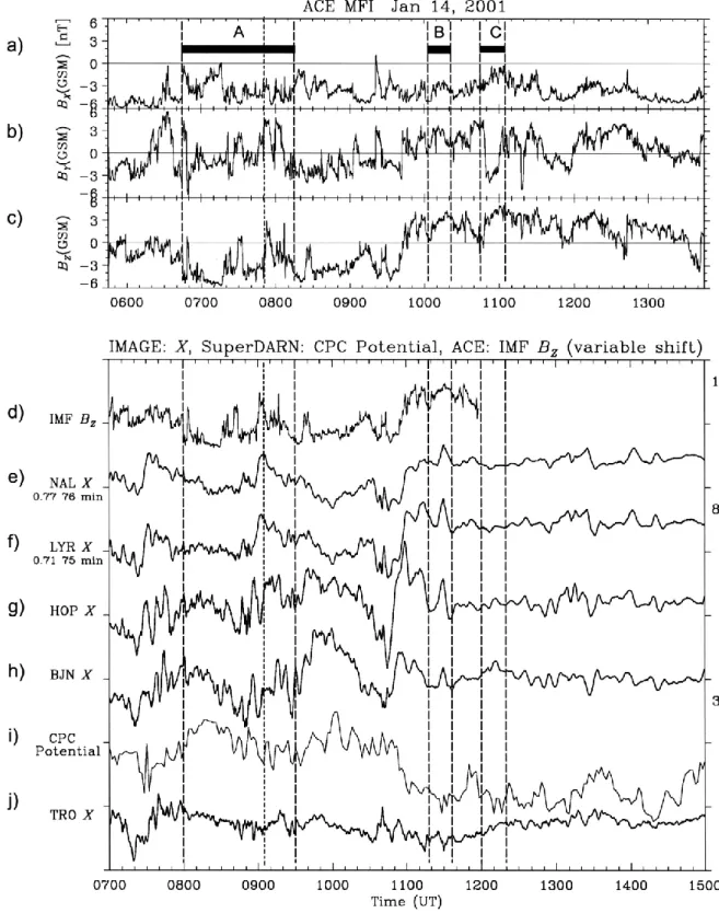
Panels (a), (b) and (c) of Fig. 3 give the three components of the IMF in GSM coordinates, as seen by the Advanced Composition Explorer (ACE) satellite near to the L1 point. Opgenoorth et al. (2001, this issue) report a very high cross-correlation of the clock angle of the magnetosheath field (in the GSE Z−Y plane), as seen by Cluster once it had emerged from the magnetosphere at about 15:00 UT, with the same an-gle seen by ACE. The conservation of clock anan-gle across the bow shock means that the correlation coefficient is very high and very significant, and the lag of peak correlation (74 min.) is a good estimate of the propagation delay between ACE and the magnetopause at 15:00 UT. In Fig. 3, we estimate the lag in a different manner for 7:00–12:00 by comparing the Z-and Y -components of the IMF, seen by ACE in GSM coordi-nates, with the X-component (northward) of the perturbation to the geomagnetic field 1BX, as seen by 5 ground-based
20 10 0 -10 -20 XGSE 20 10 0 -10 -20 YGSE 00:00 UT 2001/01/14 00:00 UT 04:00 UT 08:00 UT 12:00 UT 16:00 UT 20:00 UT 20 10 0 -10 -20 XGSE -20 -10 0 10 20 ZGSE 00:00 UT 2001/01/14 00:00 UT 04:00 UT 08:00 UT 12:00 UT 16:00 UT 20:00 UT -20 -10 0 10 20 YGSE -20 -10 0 10 20 ZGSE 00:00 UT 2001/01/14 00:00 UT 04:00 UT 08:00 UT 12:00 UT 16:00 UT 20:00 UT
Fig. 2. The Cluster orbit in Geocentric Solar Ecliptic (XGSE, YGSE,
ZGSE) coordinates (in black) along with the mapped field lines that give ionospheric footprints, such as that shown in Fig. 1. (a), (b) and (c) are projections onto the (XGSE, YGSE), (XGSE, ZGSE) and (YGSE, ZGSE) planes and the solid and dashed blue lines show the model magnetopause and bow shock locations for ZGSE = 0,
YGSE =0, and XGSE = 0, respectively, predicted using the mag-netopause model by Shue et al. (1997) and the bow shock model by Peredo et al. (1995). Traced field lines are shown from the space-craft locations at 04:00, 08:00 and 12:00 UT. Field lines mapped to the local (northern) hemisphere are shown in green, and those mapped to the southern hemisphere are in red.
magnetometers of the IMAGE chain (Syrj¨aasuo et al., 1998) at Ny ˚Alesund (NAL, Fig. 3e), Longyearbyen (LYR, Fig. 3f),
1594 M. Lockwood et al.: Coordinated observations of transient poleward-moving events Hopen (HOP, Fig. 3g), Bear Island (BJN, Fig. 3h), and
Tromsø (TRO, Fig. 3j). A correlation with the IMF BY is expected due to the Svalgaard-Mansurov effect, which is due to the magnetic curvature (“tension”) force on newly-opened field lines, and also with the IMF BZ since it controls the production of such newly-opened field lines. The maximum correlation coefficients (with corresponding lags) of BY for NAL and LYR are 0.58 (73 min) and 0.55 (72 min), respec-tively. The corresponding numbers for IMF BZ, and NAL and LYR are 0.77 (76 min) and 0.71 (75 min), respectively. Note that the use of a 3-hour sliding window shows that the lag of peak correlation varies between about 70 and 80 min. By using the Fischer-Z test for a significant difference in the correlation coefficient, we find the uncertainty in the lag at any one time is typically ±5 min. Figure 3d repeats the IMF BZ variation, this time on the same time axis as the iono-spheric measurements (parts e–k), i.e. shifted by the best-fit propagation lag of 75 min.
Figure 3 marks three periods of special interest: A, B and C. Allowing for the average lag of 75 min, these intervals correspond to 8:00–9:30 UT, 11:19–11:27 UT and 12:00– 12:20 UT, respectively, in the ionosphere. We will study pe-riod A in detail in this paper; pepe-riods B and C are the subject of a subsequent paper by Lockwood et al. (2001a, this issue). The magnetic perturbations seen on the ground show con-trol by both IMF BZand BY. In both cases, the lag is slightly longer for NAL, which is poleward of LYR, indicating a poleward motion. Deflections are considerably weaker at Tromsø, placing the open-closed field-line boundary (OCB) somewhere between there and Bear Island, which is consis-tent with particle observations by DMSP-F12 (see next sec-tion).
Figure 3 shows that throughout interval A (08:00– 09:30 UT in the ionosphere), the IMF was predominantly southward with a BZ component in GSM primarily in the range between −2 and −4 nT, with only brief northward ex-cursions. The BXcomponent is negative throughout, and the BY component is negative for the majority of this interval, but with some positive excursions. The solar wind data (not shown) reveal that the solar wind velocity Vswduring interval A was roughly constant (varying between 365 and 400 km/s, but close to 368 km/s for the majority of the time). The av-erage number density Nsw was initially 6 · 106m−3, falling to a minimum of about 2 · 106m−3(at the 08:00 observation time, 09:15 lagged time) before rising again to 5 · 106m−3 by the end of the interval. The fluctuations in the average dy-namic pressure, Psw =< mi > NswVsw2 (where < mi >is the mean ion mass) primarily follow those in Nsw and thus, also show a variation (50% about the mean of 1.1 nPa in in-terval A). Subsequently, Pswfell even further, so by intervals B and C, it was only 0.6 nPa on average; for comparison, the mode value of the overall distribution of Pswis close to 3 nPa (Hapgood et al., 1991).
Figure 3j shows the transpolar voltage deduced by fitting an IMF-dependent potential contour model to the line-of-sight velocity data from the SuperDARN radars (Ruohoniemi et al., 1989). The effect of the northward turning of the IMF
is seen just before 11:00 as a decrease in transpolar voltage and an increase in 1BXat all stations. In the 2-minute volt-age data shown in Fig. 3i, 17 peaks can be defined between 08:00 and 11:00 UT. Each can be associated with a minimum in the 1BXat BJN and HOP, and these data series give a re-peat interval of the order of 10 min (as seen in the ESR data for the same interval, see Sect. 2.3).
Figure 3 stresses that the responses to the IMF changes with a lag of 75(±5) min were seen at a range of latitudes at the MLT of the ESR and also in the transpolar voltage. It can be seen that around the time of Fig. 1 and the cusp crossing by DMSP-F12 (09:05–09:07 UT, marked by a dot-dashed line in Fig. 3), neither BY nor BZwere stable in their polarity. To within the lag uncertainty of ±5 min, we can define the appropriate average IMF conditions to have been BX= −3 nT, BY = +2 nT, BZ= −3 nT.
2.2 DMSP-F12 observations
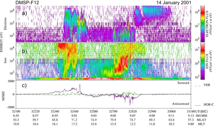
Figure 4 shows energy-time spectrograms (a) for electrons and (b) for ions, as observed by the Defense Meteorological Satellite Program (DMSP)-F12 spacecraft as it passed along the path given in Fig. 1. In both cases, the differential energy flux is plotted as a function of energy (increasing upward) and observation time. Before the satellite entered the polar cap, it passed through an auroral oval showing a series of inverted-V electron arcs at 08:59–09:02 UT. It then entered the polar cap at a magnetic latitude close to 71◦and an MLT of 17:00. The purple line in Fig. 4c shows the horizontal con-vection velocity perpendicular to the satellite track and this changed from sunward to weakly anti-sunward close to the poleward edge of this auroral oval. The satellite was then briefly within the polar cap precipitation region until about 09:03, when it began to observe mantle precipitation and at 09:05, it observed cusp ions and electrons which persisted until 09:07. The cusp was seen between magnetic latitudes of 73.7–75.9◦, over the MLT range 13:54–12.12 hrs. Within the cusp, convection flows were anti-sunward, stronger and highly structured. The green line in Fig. 4c shows that in the cusp, vertical flows were structured, pointing upward around 500 m/s, but were downward in the polar cap. The thicker segments of the pass shown in Fig. 1 mark the locations where DMSP-F12 observed the dusk auroral oval and the cusp.
The magnetosheath ions show a structured dispersion. This structure is not as straightforward as the examples pre-sented by Newell and Meng (1991), Lockwood et al. (1993b) and Pinnock et al. (1995); nevertheless, clear upward dis-continuities can be seen in the cusp ion lower cutoff en-ergy, Eic. The first major discontinuity is an upward step in Eic, consistent with a stepped cusp. This is followed by a fall and subsequent rise in Eic, which is not fully con-sistent with either a stepped or a sawtooth cusp ion signa-ture. Thereafter, the cusp takes on the classic sawtooth ap-pearance with a gradual fall in Eic followed by an upward step and then two isolated patches of the higher energy cusp ions, showing features that were all observed by Pinnock et
M. Lockwood et al.: Coordinated observations of transient poleward-moving events 1595
Fig. 3. (a) to (c) The components BX, BY and BZ of the interplanetary magnetic field (IMF) in GSM coordinates, as seen by the ACE satellite near to the L1 point. Interval A relates to the present paper, intervals B and C are studied in detail by Lockwood et al. (2001a, this issue). (d) The IMF BZcomponent shown in 3a, but here lagged by the optimum propagation delay from ACE to the dayside ionosphere of
75 min. Also shown on this time axis are the X components (northward) of the perturbation to the geomagnetic field seen by 5 magnetometers of the IMAGE chain at (e) Ny ˚Alesund (NAL), (f) Longyearbyen (LYR), (g) Hopen (HOP), (h) Bear Island (BJO) and (j) Tromsø (TRO). Panel (i) shows the transpolar voltage derived from a convection model fit to the SuperDARN data. Allowing for the lag of 75 min., intervals A, B and C correspond to 8:00–9:30 UT, 11:19–11:27 UT and 12:00–12:20 UT, respectively, in the dayside ionosphere.
1596 M. Lockwood et al.: Coordinated observations of transient poleward-moving events
DMSP-F12 14 January 2001
a)
b)
c)
Fig. 4. Energy-time spectrograms for (a) electrons and (b) ions observed by DMSP-F12 as it passed equatorward along the path given in
Fig. 1. In both cases, the differential energy flux is plotted as a function of energy (increasing upward) and observation time, ts. (c) shows
the vertical (green) and horizontal (purple) components of the ion velocity (the horizontal component is perpendicular to the satellite track such that positive values have a sunward component and negative values an anti-sunward component).
al. (1995) and modelled by Lockwood and Davis (1996). We would expect a sawtooth signature for such a longitudinal cusp pass in the presence of pulsed reconnection, unless the reconnection pulses have very small amplitude (Morley and Lockwood, 2001). The evolution of the cusp ion signature shown in Fig. 4b reveals reconnection pulses that were ini-tially small, and then subsequently grew in amplitude. The sawtooth dispersion is seen to extend to the high-energy elec-trons; magnetospheric BPS electrons were seen at energies above 1 keV at almost exactly the same time that the magne-tosheath electrons (below 1 keV) disappeared (defining the “electron edge”, Gosling et al., 1990; Onsager et al., 1993; Onsager and Lockwood, 1997). However, these BPS elec-trons subsequently disappeared again in a dispersed manner (higher energies disappearing first) before reappearing, at all energies simultaneously, just after 09:08. Although not un-common in cusp ions, this is the first time that such a saw-tooth signature has been reported to extend into electron data: it is clearly seen in this case due to of the increasing ampli-tude of the reconnection pulses, with the pulse that provides the electron sawtooth representing the largest of the series. Given that electrons travel very quickly down field lines, we can identify the location of the electron edge as very close to the open-closed boundary (OCB) (see Lockwood, 1997a); the onset of energetic magnetospheric electrons marks the passage of the satellite from open to closed field lines. The
OCB then erodes equatorward in response to a reconnec-tion pulse which is sufficiently large enough in amplitude to cause the OCB to overtake the satellite. This, in turn, causes the electrons to disappear, with the most energetic electrons escaping first through the magnetopause. Subse-quently, the equatorward motion of the OCB slowed, allow-ing the satellite to overtake it again, and causallow-ing the BPS electrons to reappear at all energies. These data not only show that reconnection was pulsed, but also show the loca-tion of the OCB near 12:00 MLT oscillating in invariant lati-tude between 71.5◦and 73.7◦in the interval 09:07– 9:08 UT. This places the ESR field-aligned beam (at invariant latitude 75.1◦) on open field lines within (but near the poleward edge) the cusp, as seen by DMSP-F12.
2.3 EISCAT Svalbard radar observations
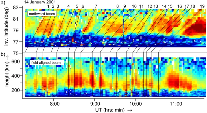
Figure 5 shows 2-minute post-integrations of the ESR radar observations of plasma concentration in the interval 07:15– 11:45 UT. The top panel is for the low-elevation northward beam and the lower panel is for the field-aligned beam; the plasma concentration is contoured as a function of invariant latitude and observation time in the top panel, and as a func-tion of altitude and observafunc-tion time in the lower panel. (The contour level scales used are the same as in Fig. 6a). The poleward-pointing beam observed a series of high-density
M. Lockwood et al.: Coordinated observations of transient poleward-moving events 1597
83
81
79
77
75
600
400
200
hei
ght (
km)
→
inv. la
titude
(deg)
northward beam8:00 9:00 10:00 11:00
UT (hrs: min)
→
field-aligned beam 1 2 3 4 5 6 7 8 9 10 11 12 13 14 15 16 17 18 19 14 January 2001a)
b)
Fig. 5. Two-minute post-integrations of the ESR radar observations of plasma concentration in the interval between 07:15–11:45 UT. (a)
is for the low-elevation, northward beam and (b) is for the field-aligned beam, and the plasma concentration is contoured as a function of invariant latitude and observation time in the top panel and as a function of altitude and observation time in the lower panel. (The contour levels are given by the scale shown for the top panel of Fig. 6). Lines map the centres of poleward-moving events seen in the low-elevation beam back to the invariant latitude of 75.1◦of the field-aligned beam.
plasma regions (polar cap “patches”) moving along the beam to higher latitudes. These are similar to those seen by lower-latitude radars (Chatanika and the EISCAT UHF and VHF mainland radars), using similar modes of operation with poleward-pointing beams at low elevation, but only when the polar cap is considerably expanded (e.g. Foster and Doup-nik, 1984, Lockwood and Carlson, 1992). Since their pole-ward phase motion was roughly constant in speed, a straight line can be placed through each of these events. These lines have been mapped back to an invariant latitude of 75.1◦, rep-resenting the location of the field-aligned ESR beam. Fig. 5 shows that the events seen in the field-aligned beam gener-ally match those subsequently seen propagating poleward in the low-elevation beam. The relationship of similar events in the ESR field-aligned beam to phenomena, such as poleward moving flow channels seen by the CUTLASS HF radar and poleward-moving 630 nm auroral transients, has been stud-ied by McCrea et al. (2000) and Lockwood et al. (2000).
This match between the plasma concentration data seen in the two ESR beams persists until the first effects of the northward turning of the IMF, shown in Fig. 3, reaches the magnetosphere at around 10:45. Thereafter, the signatures do not correspond and they do not share a common origin (Blelly et al., 2001, private communication). While patches are passing over both beams, the field-aligned beam gives a detailed picture of the altitude profile of the plasma
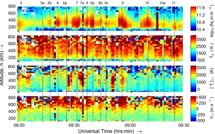
param-eters in each event as it passes over the radar, as presented in Fig. 6. These data have a lower post-integration time of 1 min which is the optimum compromise between the time resolution and the signal-to-noise ratio for the field-aligned beam. The altitude profiles of the events show that most of the plasma concentration (Ne) enhancements were primarily above 150 km (top panel Fig. 6); this altitude corresponds to about 76.5◦ invariant latitude for the poleward-pointing beam and thus, the events are not generally seen at lower latitudes since the low elevation beam is underneath the Ne events close to the radar. Similarly, the enhancement is small above about 600 km and so altitude effects also indicate that events are not generally detected at invariant latitudes above about 82◦. By taking the time series of the data observed in the range gate of the two beams that are at a 300 km altitude, and cross-correlating with a 1-hour running window, gives cross-correlation coefficients between 0.75 and 0.9. (These fall to lower values if longer windows are used due to of the variations in the poleward phase speed of the events).
The lower panels of Fig. 6 show the electron tempera-ture, Te, the field-aligned ion temperature [Ti]kand the field-aligned ion velocity, Vk. The electron temperatures, Te, seen in the field-aligned beam were higher and more structured when the IMF was southward (average values at 300 km, for example, were about 3000 K, compared to about 1500 K af-ter 11:00, when the IMF was predominantly northward (see
1598 M. Lockwood et al.: Coordinated observations of transient poleward-moving events V | | (m s –1 ) [ T i ]| | ( K ) T e ( K ) lo g10 (N e in m –3 )
Altitude
, h (
km)
→
08:00 08:30 09:00 09:30Universal Time (hrs:min)
→
800 600 400 200 800 600 400 200 800 600 400 200 800 600 400 200 11.6 11.2 10.8 10.4 3500 2500 1500 500 3000 2000 1000 0 +500 +250 0 -250 -500 5 5a 5b 6 6a 7 7a 8 8a 8b 8c 9 10 10a 11 a) b) c) d)
Fig. 6. One-minute post-integrations of the data from the field-aligned ESR beam for 08:00–09:30. Altitude profiles are shown for (from
top to bottom): (a) the plasma concentration, Ne; (b) the electron temperature, Te; (c) the field-aligned ion temperature, [Ti]kand (d) the
field-aligned (line-of-sight) ion velocity, Vk. The dashed lines mark the centre of events 5, 6, 7, 8, 9, 10, and 11 in this interval, as defined in
Fig. 5. These higher-resolution Nedata in the field-aligned direction reveal additional events 5a, 5b, 6a, 7a, 8a, 8b, 8c, and 10a.
Opgenoorth et al. 2001, this issue). The parallel ion tem-peratures, [Ti]k, showed brief transient enhancements (up to 3000 K, compared with to the background level of 1300 K) and persistent fast, upward flows (with speeds Vkof 300 m/s or more at 500 km) were also observed, but when the IMF was southward.
The ion temperature behaviour is dominated by the largest two terms in the ion thermal balance equation (Lockwood et al., 1993d; McCrea et al., 1993) such that the field-parallel ion temperature is:
[Ti]k=Tn+ βkmn
2k |V − U |
2, (1)
where Tnis the temperature and mnis the mean mass of the neutral gas atoms/molecules; βkis the temperature partition coefficient; k is Boltzmann’s constant; V and U are the ion and neutral gas velocity vectors, respectively. The coefficient βkhas a minimum value of zero (the “relaxation model” of ion-neutral collisions which would be valid for charge ex-change with no momentum exex-change) and a maximum value of 2/3 (for isotropic scattering). A lower βk corresponds to a higher temperature anisotropy. McCrea et al. (1993) found that βkwas about 1/3 near 300 km, but rose to values closer to 2/3 at greater altitudes since the isotropising effects of ion-ion collision-ions became as important as the anisotropic heating effect of ion-neutral collisions. At the highest altitudes, heat
conduction from the electron to the ion gas may become im-portant since electron temperatures are generally higher. The fact that βk>0 means that differences between V and U re-sult in rises in [Ti]kthat can be detected by the field-aligned ESR beam. Recently, Lockwood et al. (2000) have stud-ied ESR observations of ion heating in and around transient poleward-moving events, as seen by optical instruments and the CUTLASS HF radars. They found that the behaviour de-pends on the time in the evolution of events at which the radar intersects them. This occurs because the enhanced ion flows V in the events evolve as they change from moving longitudi-nally under the magnetic curvature force (“tension”), associ-ated with the IMF BY component, to poleward motion under the influence of the solar wind flow (Lockwood et al., 1989a, b), whereas the neutral flows U can only show an average response to these changing ion flows. This introduces great variability into the ion temperatures caused by ion frictional heating, even if the interplanetary conditions are stable.
In the interval 07:15–10:50, 19 poleward-moving events were seen in the 2-min resolution data from the field-aligned ESR beam (Fig. 5), all of which can be subsequently iden-tified in the poleward-pointing beam. This gives an average repetition interval of the order of 10 min. Figure 6 shows the 1-min integrated data for the field-aligned beam for the interval A, and an additional 8 events can be seen in these
M. Lockwood et al.: Coordinated observations of transient poleward-moving events 1599
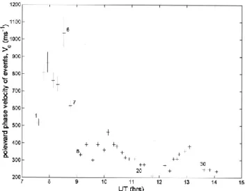
Fig. 7. The phase velocity of the poleward motion of the events, Ve
(from the slope of the fitted lines in the top panel of Fig. 5). The events are plotted at the time that they are at invariant latitude of 79◦and selected events have been numbered for comparison with Fig. 5. Events after 11:00 (21–32) are discussed by Lockwood et al. (2001a, this issue).
higher-resolution data (labelled 5a, 5b, 6a, 7a, 8a, 8b, 8c, and 10a). Of these, event 7a appears to be caused by a bad fit to the data; it is only present in one post-integration period, The altitude profile in Neis unlike that in any other event and anomalous values are also seen in Te, [Ti]kand Vk. Neglect-ing 7a means that we identify a total of 14 events in these data in interval A, giving a mean repeat period of 6.4 min, which is considerably less than the 10 min derived from the 2-min integrated data and from the poleward beam.
Figure 6 reveals that the signatures in the various parame-ters measured (Ne, Te, [Ti]kand Vk) have complex relation-ships and indicate that a number of factors may have con-tributed to the observed structure in the plasma concentra-tion. Events 6, 8a, 8c,10 and 10a show decreases in electron temperature Te coincident with the rises in Ne. Events 8b, 8c and 9 show (generally weak) simultaneous rises in field-parallel ion temperature [Ti]k. However, the major rises in [Ti]kare between events (e.g. between 6a and 7, 7 and 8, 8c and 9). Event 9 (which shows high Ne, Teand [Ti]k) reveals a strong burst of upflow velocity, Vk, and hence, ion flux NeVk. Figure 7 plots the phase velocity of the poleward motion of the events, Ve (from the slope of the fitted lines in the top panel of Fig. 5). The events are plotted at the time that they are at an invariant latitude of 79◦ and selected events have been numbered for comparison with Fig. 5. Events after 11:00 (21–32) are discussed by Lockwood et al. (2001a). It should be noted that three factors enter into the values of Ve: the poleward convection speed, the orientation of the events and the east-west convection speed. Thus, Ve depends on both the BY and BZ components of the IMF, and the orien-tation of the events will evolve systematically as the radar moves from near noon in MLT into the mid-afternoon sector.
2.4 Magnetometer observations
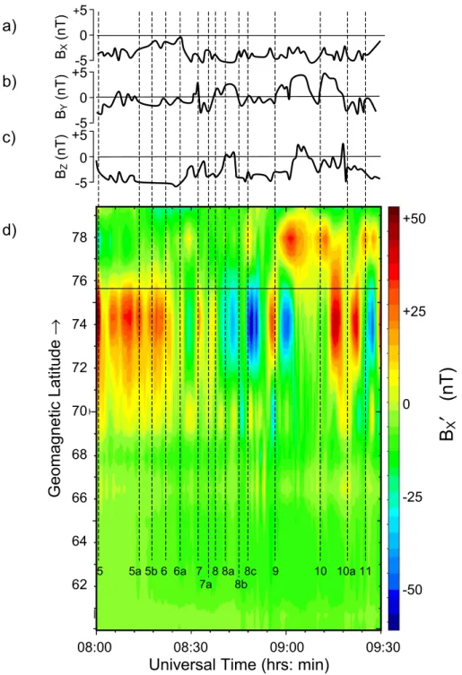
Figure 8d shows the “upward continuation” of the X-com-ponent of the magnetic field BX0 (derived as a function of latitude from the IMAGE magnetometer chain). The tech-nique used employs Fourier analysis of the data from the lat-itudinal chain of stations on the ground to reconstruct high-resolution latitude variations that would have been observed just below the current layer (Mersmann et al., 1976). A pos-itive X-component (northward) is a response to an eastward current. If the magnetometers are responding to a Hall cur-rent in the E-region (i.e. if horizontal stratification of con-ductivities can be assumed), this corresponds to a westward convection velocity in the F-region. Note that the yellow and red colours reveal positive BX0(eastward current), whereas green and blue reveal negative BX0(westward current). Parts (a), (b) and (c) of Fig. 8 give the lagged (by 75 min) varia-tions of the IMF components in the GSM reference frame. The dashed lines give the events identified in Fig. 6. The horizontal line is the latitude of the field-aligned ESR beam. Note that all events were seen while the IMF was southward. Between 8:00 and 8:25 (roughly 10:45–11:10 MLT), weak westward current was seen poleward of a stronger eastward current. In this interval, the lagged IMF was strongly south-ward with a weak negative BY component. Thus, this is con-sistent with the magnetometer chain spanning the convection reversal of the dawn cell for IMF BY <0. Note that the cur-rents were not steady – 5 enhancements seen in the eastward current during this 25 min. In this interval, events 5a, 5b and 6 were identified from the radar data, however, no clear cor-respondence with the BX0variations is apparent.
Between 08:25 and 09:30, BX0oscillated between this sit-uation (westward current poleward of eastward current) and the reverse situation (eastward current poleward of westward current). The latter is consistent with the chain straddling the convection reversal of the dawn cell for IMF BY > 0. The IMF data reveal several reversals of the polarity of IMF BY in this interval. For 09:03–09:19, the current is east-ward at all latitudes, consistent with the chain moving into the dusk cell for IMF BY > 0. The plasma concentration (Ne) enhancement events seen by the ESR in this interval can all be associated with either oscillations in the form of the BX0latitude variation or with a transient enhancement of BX0. Thus, there is structure in the detected currents that is broadly associated with the Ne events, although the associ-ation is not straightforward since the BX0 signatures have a variety of forms. This is perhaps not surprising considering the variations in IMF BY and BZ(Fig. 3), and the effects this will have on BX0. In addition, the competing effects of mag-netosheath precipitation, the enhanced loss rates associated with ion-neutral frictional heating and the effect of event evo-lution (Lockwood et al., 2000) will introduce variations into the form of the Neevents; this fact is reflected in the range of behaviours of Te, [Ti]kand Vkduring the Neenhancements.
1600 M. Lockwood et al.: Coordinated observations of transient poleward-moving events 5 5a 5b 6 6a 7 8 8a 8c 9 10 10a 11 7a 8b BZ ( n T) B Y ( n T) B X (n T)
B
X′ (nT)
+50 +25 0 -25 -50 +5 0 -5 +5 0 -5 08:00 08:30 09:00 09:30Universal Time (hrs: min)
78 76 74 72 70 68 66 64 62 +5 0 -5
Geomagneti
c Latitu
de
→
a)
b)
c)
d)
Fig. 8. (a) to (c), the lagged (by
75 min) variations of the IMF compo-nents BX, BY and BZin the GSM ref-erence frame. (d) the “upward continu-ation” of the X component of the mag-netic field, BX0, as a function of latitude
from the IMAGE magnetometer chain. The technique used to derive BX0
em-ploys Fourier analysis of the observa-tions of the data from the latitudinal chain of stations on the ground to re-construct high-resolution latitude vari-ations that would have been observed just below the current layer. The ver-tical dashed lines give the times of the peaks in the Neevents defined in Fig. 6.
2.5 Convection observations
Figure 1 shows a 5-min integration convection pattern in an invariant latitude (3), with the MLT frame at 09:05. This has been derived by the AMIE technique, employing magne-tometer, SuperDARN, DMSP and ESR observations. This is the time of the closest approach of the DMSP-F12 satellite to the ESR and marks the start of the cusp intersection (cusp ions are seen at 09:05–09:07 and the electron edge is encoun-tered three times during the interval 09:07–09:08). The flows show a southward IMF flow pattern, with a transpolar voltage of 54 kV. A similar value for the transpolar voltage and flow
pattern is obtained for this time using model fitting to Super-DARN line-of-sight velocity data (Ruohoniemi et al., 1989, Ruohoniemi and Baker. 1998). The flow in the cusp region is directed towards dawn (westward), which is characteristic of a positive IMF BY for these northern hemisphere data (e.g. Heelis et al., 1984). With the inferred lag of 75 min for this interval, the relevant IMF data were recorded by ACE at 7:50. Figure 3 shows that the IMF BY component in GSM was in-deed positive at this time, with negative IMF BZ. At other times in interval A, the IMF BY was weakly negative and then the flow streamlines in the dayside polar cap were close to poleward with only a small eastward component. At such
M. Lockwood et al.: Coordinated observations of transient poleward-moving events 1601 times, the flow streamlines that passed over the ESR were
closer to Cluster than seen in Fig. 1, in which the path of the DMSP-F12 satellite in this (3) - MLT frame is also plotted. The thicker segments of the path mark where the DMSP-F12 was in the dusk auroral oval (observing a sunward flow) and in the cusp (observing a structured anti-sunward flow). While within the polar cap, between these two segments, DMSP-F12 observed weak anti-sunward flow (see Fig. 4). The flows are consistent with the inference from the upward continua-tion magnetic disturbance, BX0, as plotted in Fig. 8, with an eastward current at all latitudes showing that the magnetome-ter chain is in the dusk convection cell at this time. However, the BX0variation before and after the pass reveals the chain moving out of, and then back into a dawn cell. This is con-sistent with the zero-potential contour between the two cells lying close to the meridian of Svalbard, as seen in Fig. 1, where the locations of the two ESR beams can also be seen. Convection is poleward, consistent with the poleward phase motion of the events, but at this time, it has a westward com-ponent that is of the same order of magnitude as the poleward flow.
Figure 9 summarises some of the line-of-sight flow ob-servations made on the dayside at a 2-min resolution by the SuperDARN radars. Each part shows a map of the dayside in geographic coordinates with noon at the top and the day-night terminator as shown. The vectors shown point along the beams where scatter was observed, and they have a length and polarity that is scaled according to the line-of-sight ve-locity. They are also colour-coded according to the magni-tude of the observed line-of-sight velocity. Note that these are not 2-dimensional convection vectors. The DMSP-F12 pass is shown in the same format as Fig. 1, with the addi-tion of a red arrow that gives the locaaddi-tion of the satellite at that time. The yellow dot is the field-aligned ESR beam. At 09:01 UT (Fig. 9a), enhanced flows are seen in the polar cap (in red) and this patch subsequently migrates anti-sunward and fades in magnitude and size. A small patch of enhanced poleward flow is seen around the ESR. This has faded by 09:05 (Fig. 9b) but another patch to the west of the radar has appeared by 09:09 (Fig. 9c). This subsequently spreads east-ward over the ESR (09:17, Fig. 9d). Note that the lagged IMF data shows positive IMF BY for almost all of the inter-val covered by Fig. 9 (Fig. 3) and the vector flow in the cusp is correspondingly westward (Fig. 1). Thus, the eastward ex-pansion is not due to the curvature force on newly-opened field lines and is likely to reflect an eastward expansion or motion of the reconnection X-line. A decay in this enhanced flow starts near noon and spreads both east and west, such that by 09:21 (Fig. 9e), the enhanced flows are seen only in the mid-morning and mid-afternoon sectors. This behaviour is as predicted by Lockwood (1994) for an active X-line that forms near noon and then expands and bifurcates, giving ac-tive segments travelling toward both dawn and dusk. The data also reveal a convection reversal boundary (CRB), seen as a reversal of the line-of-sight flow from toward to away from the radar. This is near 75◦in the morning sector and close to the satellite pass in the afternoon. By 09:27 (Fig. 9f),
the enhancement is not seen at all, and the CRB has migrated poleward in the morning sector, but not in the afternoon sec-tor.
2.6 Global auroral observations
The flow streamlines in Fig. 1 are superposed on the relevant global auroral image taken by the Wideband Imaging Cam-era (WIC) of the FUV instrument on the IMAGE spacecraft (Mende et al., 2000). This imager covers the ultraviolet range of wavelengths between 140 and 180 nm with temporal reso-lution of 2 min. The original image was taken from a geocen-tric distance of 50 200 km and was remapped to a local time and geomagnetic latitude grid. The UV aurora is primarily observed in the regions of upward field-aligned current asso-ciated with the pattern of convection (the region 2 at dawn, on the equatorward edge of the convection boundary, and the region 1 at dusk, close to the convection reversal boundary). The DMSP-F12 satellite is poleward of the auroral oval when in the region defined as the polar cap from the precipitation characteristics.
The WIC camera is primarily sensitive to aurora created by electron precipitation, which when measured by DMSP in the cusp, showed very low characteristic energy (below 300 eV) and when combined with the small differential en-ergy flux, this precipitation only produced a very weak signal from the cusp region. Even the electron precipitation mea-sured by DMSP at around 09:09 with higher characteristic energies (several keV) was not intense enough and a gap ap-peared in the dayside aurora. The FUV instrument on IM-AGE also contains the Spectrographic Imager (SI12) chan-nel, which measures the Doppler shifted Lyman-alpha emis-sion from precipitating protons (Mende et al., 2000). This imager is sensitive to emission from protons with at least 2 keV energy. The high energy tail of the differential ion energy flux (primarily protons) measured by DMSP created only a very weak signal in the proton aurora imager from the cusp (not shown). At the first crossing of the auroral oval by DMSP at about 71◦ magnetic latitude and 17:00 MLT (see Sect. 2.2), the UV images confirm the location of the proton precipitation equatorward of the most intense inverted V-like electron precipitation.
2.7 Cluster observations
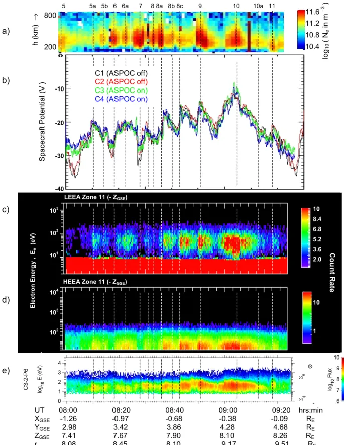
Figures 10b to 10e shows plasma observations made during interval A by the Cluster spacecraft, and Fig. 10a reproduces the Ne variation shown in Fig. 6a, shifted in time to obtain the best agreement (see below). Figure 10b shows the space-craft potential from the EFW instruments on all 4 spacespace-craft, a measure of the plasma concentration around the spacecraft. The spacecraft potential was held almost constant by the AS-POC instruments which were active on spacecraft C3 and C4. However, close inspection revealed that for this case with very low ambient plasma concentrations, the potential of C3 and C4 still varied about the almost constant value due to the ambient plasma concentration variations.
Cross-1602 M. Lockwood et al.: Coordinated observations of transient poleward-moving events
a) b)
c) d)
e) f)
Fig. 9. SuperDARN observations of the line-of sight plasma velocities seen at 09:00–09:30. Selected frames are for 2 min scans centred on: (a) 09:01, (b) 09:05, (c) 09:09, (d) 09:17 (e) 09:21, and (f) 09:27. The orbit of DMSP-F12 is shown in each case, with the auroral oval and
cusp locations marked: the red arrow gives the location of the satellite in each case. The ESR field-aligned beam is shown as a yellow dot.
correlation of the potential values seen on these spacecraft (C3 and C4) with an average of those seen by C1 and C2 (on which ASPOC was off) showed a systematic variation with only small scatter. Fitting the scatter plot with an exponential variation gives an excellent fit in both cases and this was used to scale the data by C3 and C4, taken with ASPOC turned on, into the values that would have been seen had ASPOC been turned off. Fig. 10b shows that the four spacecraft saw fluc-tuations in the plasma concentration in roughly 10-min time scales (9 in 90 min) that were almost identical, indicating that the plasma structures were considerably larger than the inter-craft separations of the order of 600 km.
Parts (c) to (e) of Fig. 10 analyse the nature of these plasma
concentration structures using data from spacecraft C3. Fig-ures 10c and 10d show the data from the LEEA and HEEA detectors on the PEACE instrument, respectively. In both cases, the particles seen are in zone 11 of the detector, which makes continuous observations of electrons moving in the +ZGSEdirection. The ASPOC instrument held the spacecraft
potential such that the photoelectrons were seen by LEEA up to only 10 V (photoelectrons seen by the spacecraft with ASPOC turned off extended up to about 30 eV in the LEEA data). Fig. 10e shows the ion observations made by the CIS instruments on board C3 (R`eme et al., 1997, 2001, this is-sue). Increases in the fluxes of ions and high-energy elec-trons were seen co-incident with the low-energy electron
in-M. Lockwood et al.: Coordinated observations of transient poleward-moving events 1603
a)
b)
c)
d)
e)
lo g10 ( N e in m –3 ) 11.6 11.2 10.8 10.4 800 200 5 5a 5b 6 6a 7 8 8a 8b 8c 9 10 10a 11 h (km) → 244s 150s UT 08:00 08:20 08:40 09:00 09:20 hrs:min XGSE -1.26 -0.97 -0.68 -0.38 -0.09 RE YGSE 2.98 3.42 3.86 4.28 4.68 RE ZGSE 7.41 7.67 7.90 8.10 8.26 RE r 8.08 8.45 8.10 9.17 9.51 RE E le ct ron E n e rgy , E e (eV) Count RateLEEA Zone 11 (- ZGSE)
HEEA Zone 11 (- ZGSE) 103 102 101 104 103 102 10 8.4 6.8 5.2 3.6 2.0 10 1 Spacecr a ft P o te nti a l ( V ) C1 (ASPOC off) C2 (ASPOC off) C3 (ASPOC on) C4 (ASPOC on) -10 -20 -30 -40
Fig. 10. From top to bottom: (a) the electron concentration observations by the field-aligned ESR beam, as shown in the top panel of Fig. 6,
but shifted to earlier times to make events 5 and 11 agree. (b) potential measurements for all 4 spacecraft from the EFW instrument. (c) electron observations made by the HEEA detector of the PEACE instrument on the Cluster spacecraft 3 (C3); (d) electron observations made by the LEEA detector of the PEACE instrument on C3. In both (b) and (c), the particles seen are in zone 11 of the detector, which makes continuous observations of electrons moving in the +ZGSEdirection. (e) ion observations made by the CIS instruments on board Cluster C3.
1604 M. Lockwood et al.: Coordinated observations of transient poleward-moving events creases. Events in both ion and electron data show relatively
sudden onsets, followed by a slower decay. Figure 10c shows that the fluxes of lowest energy magnetosheath electrons seen by LEEA (10–30 eV) are quite strongly modulated during the events, and the lowest energy at which significant fluxes of such electrons are seen falls as the plasma concentration rises.
In comparing the plasma concentration structures seen by the ESR and by the Cluster spacecraft, several points must be remembered. In the 1.5 hours shown, the ESR moves in MLT from near 10:45 to 12:15, while Cluster remains close to 15:00 MLT. Conversely, the ESR remains at an invariant latitude of 75.1◦, while Cluster moves from near 85◦to 79◦. Thus, the separation of the two decreases by 1.5 hours in MLT and by about 6◦ in invariant latitude. Thus, we do not expect the propagation delay of any events that pass over both to be constant, although it might vary approximately linearly. Second, Cluster traverses much of the mantle in this period and plasma concentrations increase correspond-ingly, whereas the difference in latitude between the ESR and the open-closed boundary does not appear to drift very much. Thus, it is not surprising that events become succes-sively larger in amplitude in the Cluster data, but this trend is not found in the ESR data. In Fig. 10, the ESR data have been shifted forward in time by a lag that varies linearly with time. The end of event 5 is matched up to the end of an event at 08:00 in the EFW data, and the small event 11 is matched up to the small event in the EFW data. This yields a lag of 150 s at 08:00 and a lag of 244 s at 09:00 and gives an excel-lent match for events 9 and 10 in the Cluster data, and events 8a and 7 are seen in the Cluster data but the lag appears to be slightly overestimated. Between events 8c and 9 is an event seen by EFW, but absent in the ESR data; however, inspec-tion of Fig. 6 reveals that [Ti]k is strongly elevated at this time, indicating that the ionospheric enhancement may have been countered by enhanced plasma loss rates due to the fast plasma flow. Similar considerations apply to the minima be-tween events 7 and 8 and bebe-tween events 6a and 7, and agree-ment for events 6a to 8 is not very close.
The centre times of the ESR events are marked with dashed lines, as in Figs. 6 and 8. Given the changing sep-aration between ESR and Cluster, and the complications as-sociated with flow enhanced ionospheric loss rates, the data suggest a surprising correspondence between the two data sets.
3 Discussion
The period studied here (08:00–09:30) reveals a series of events with a repeat interval of the order of 10 min in a variety of data sets. Higher resolution data reveals further (smaller) events providing a repeat period of about 6.5 min. These values are similar to the average for the distribution of repeat periods for dayside auroral transients (Fasel, 1995), magnetopause FTEs (Lockwood and Wild, 1993), poleward-moving cusp/cleft flow channels seen by HF radar (Provan
and Yeoman, 1999; McWilliams et al., 2000) and polar cap patches (Sojka et al., 1994). Thus, they are consistent with a characteristic quasi-periodicity that is seen throughout the re-gion of dayside open field lines (cusp/cleft, mantle and polar cap). The pass of the DMSP-F12 satellite around 09:05 UT reveals that the cusp and the electron edge were equatorward of both ESR radar beams, which were both on open field lines. Events were seen in the ionospheric plasma density in both beams; they were moving poleward along the low-elevation beam and by mapping these back in latitude when the IMF was southward confirms that the same events were seen as they passed through the field-aligned beam. Compar-ison with high-resolution magnetometer data indicates that there are associated changes in ionospheric currents and con-vection, but these vary in their nature, almost certainly due to changes in the IMF BY and BZ. The events were seen by the ESR after only a very small lag following the corresponding enhancements of electron (and to a lesser extent ion) concen-trations in the mantle region of the tail lobe, as monitored by Cluster. The surprising result, therefore, is that there appears to be signatures of polar cap patches in the tail lobe particle populations, as well as in the ionosphere.
3.1 IMF control of events
Figure 3a shows that the IMF at ACE was predominantly southward until 09:45, and we can identify the effects of the northward turning at this time with the change in the ground-based magnetometer data (as shown in Fig. 3b for the IM-AGE chain, but also found in the Greenland magnetometer chain) at 11:00, consistent with the inferred propagation lag of 75 min at this time. The SuperDARN radar network also revealed a drop in the transpolar voltage following the north-ward turning (Fig. 3i). Thus, the events seen by the ESR before 11:00 are for predominantly southward IMF condi-tions. Brief periods of northward IMF were seen at ACE at 07:29–07:32 and 07:51–07:54 which applying the 75 min lag gives times of 08:44–08:47 and 09:06–09:09. These intervals do not appear to change the occurrence of the events seen by the radar; however, at these times, between events 6 and 8, there is a marked slowing in the phase speed of the poleward motion of the events. This is clearly reflected in the phase ve-locity of the poleward motion of the events, Ve (Fig. 6). Al-though event velocities do generally decrease following the arrival of northward IMF turnings at 08:45 and 10:45, there is no good overall correlation with IMF BZ. The IMF Bx was negative throughout interval A, with BY negative for the majority of the interval (between −3 and −1 nT) with a few excursions to positive BY (to about +4 nT).
Strong ion-neutral frictional heating (high [Ti]k) is seen between some of the enhanced plasma concentration Ne events, in particular, between events 6a and 7, 7 and 8, and 8c and 9. Figure 8 shows that these are associated with changes in the direction of the east-west current, as inferred from the upward continuation northward magnetic field BX0, which, in turn, can be associated with changes in the polarity of the IMF BY component.