Centre de Recherche en Economie Publique et de la Population
R
E
P
P
W
o
rk
in
g
P
ap
er
S
er
ie
s
CREPP WP No 2011/06
A Calibrated Growth Model of Global Imbalances
Lionel Artige Laurent Cavenaile May 2011
CREPP - Centre de recherche en Economie Publique et de la Population Boulevard du Rectorat 7 (B31)
A Calibrated Growth Model of Global Imbalances
Lionel Artige
∗†HEC - University of Li`ege
Laurent Cavenaile
HEC - University of Li`ege
May 7, 2011
Abstract
Global imbalances are considered as one of the main culprits of the financial crisis which started in the United States in 2007. This paper aims to build and calibrate a two-country growth model with overlapping generations to investigate the effect of a ”global saving glut” on the current account balance of the developed and developing economies. Calibrated on IMF data and forecasts between 1981 and 2016, the model rightly predicts the reversal of current account balances observed at the end of the 1990s and the disappearance of global imbalances for the period 2017-2034. This paper then studies the impact of global imbalances on the world interest rate and on the welfare of the young and old generations in the short and long run.
Keywords: Balance of payments, Global imbalances, Growth, Overlapping gen-erations
JEL Classification: E20, F21, F43, O16, O41
∗L. Artige acknowledges the financial support of the Banque Nationale de Belgique.
†Corresponding author: HEC - Universit´e de Li`ege, Economics department, Boulevard du Rectorat
1
Introduction
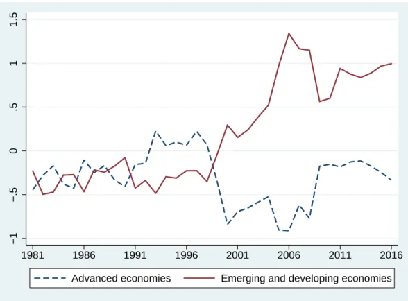
Among the factors leading to the major financial crisis which started in the United States in 2007, some point to the persistence of large global imbalances for a decade before the meltdown (Figure 1).1 By global imbalances it is meant that the fast-growing emerging
economies and the developing countries finance the current account deficits of the slow-growing advanced economies.2 This is an anomaly. Countries with a young population
and high economic growth rates, as is the case with emerging economies, are expected to experience current account deficits that can be financed by foreign saving seeking high-yield investments. Advanced economies with ageing populations and low growth prospects are expected to save more and, hence, experience current account surpluses. Saving is thus allocated where it is most productive and imbalances in current accounts reduce as diminishing returns on capital curb the growth rates of emerging economies over time. This international self-equilibrium market mechanism is ineffective when the advanced economies offer safer stores of value for the saving of the export-led developing world and thus finance their growth and their external deficits, as has been the case since 1996.3
Large current account imbalances already occurred in the past, as in the 1980s, but they were limited to the developed economies. Nowadays, they are truly global, involve rich and developing countries, and their size is a serious challenge for the stability of the world economy.4 This is the result of the political and economic changes of the last twenty
years. The integration of the countries of the former Soviet Bloc into the world goods and capital markets and the international integration of capital markets have created a huge global capital market. In this international capital market, global imbalances such as those observed since 1996 can now occur. Some have expressed concern regarding the systemic risks these global imbalances could create for the world economy ((IMF 2005), (Krugman 2007) and (Obstfeld and Rogoff 2007)). (Bernanke 2005; Bernanke 2007) expresses greater confidence regarding the ability of the market to gradually resolve the external imbalances.
The origins of these global imbalances are also debated. (Bernanke 2005) challenged the common view that was held at the time that the large U.S. current account deficit was due to the U.S. economic policies responsible for the low domestic saving and the frenzied
1This question is controversial. For instance, (Bernanke 2009), (BIS 2009), (Obstfeld and Rogoff
2009) and (Portes 2009) argue that the global imbalances played a major role in the recent financial crisis. (Blanchard and Milesi-Ferretti 2010) think that the failures of the financial system are the trigger for the financial crisis and contributed to the widening of global imbalances. (Laibson and Mollerstrom 2010) and (Whelan 2010) challenge the link between global imbalances and the financial crisis.
2This definition reflects the pattern of global imbalances currently observed but global imbalances
could result from the current account deficits and surpluses of any groups of countries. In the 1980s, current account imbalances involved mainly advanced economies, namely the U.S. and Japan.
3(Blanchard and Milesi-Ferretti 2010) show that the ratio of the absolute value of the world current
account balances to the world GDP was stable from 1970 to 1996 and started to increase sharply from then on.
4In fact, the current global imbalances are mainly a current account imbalance between the United
−1 −.5 0 .5 1 1.5 1981 1986 1991 1996 2001 2006 2011 2016
Advanced economies Emerging and developing economies
Source: IMF, World Economic Outlook, April 2011 Country groups information: see IMF 2011 WEO database. IMF estimates for data after 2010.
Figure 1: Current account balance as a percentage of world output (1981-2016)
consumption of foreign goods. He argued that the reversal in the current account positions of the emerging economies in the second half of the 1990s created a “global saving glut” allowing the cheap financing of the U.S. current account deficit and accounting for both the widening of global imbalances and the low level of real interest rates. Bernanke puts forward several reasons to explain this reversal. First, many developing and emerging economies modified their economic policies after the series of financial crises in the 1990s so as to yield current account surpluses and build foreign exchange reserves in order to reduce the financial liquidity risk in case of a sudden change in foreign investors’ behavior. Second, other countries, such as China, maintained their export-led growth policy by preventing their currency from appreciating. Third, the rise in oil prices during the last decade inflated the income of oil-exporting countries and, hence, increased their level of saving. Finally, the deep and liquid U.S. financial markets provided a highly attractive heaven for this foreign saving glut. All these factors contributed to increasing saving in developing countries and enabling the U.S. and other industrial countries to afford to live on credit. In order to account for global imbalances, (Caballero, Farhi,
and Gourinchas 2008) add to Bernanke’s hypothesis the underdevelopment of financial markets in emerging countries. In their model, increasing saving in emerging countries does not find sufficient sound local stores of value and, therefore, a rising proportion of saving flows to the perceived better U.S. financial markets. Thus, the widening of the U.S. current account deficit, the decline in world interest rates and the increase in U.S. assets within global portfolios are not an anomaly but rather a global equilibrium resulting from the capital flows in asset markets. The “global saving glut” hypothesis has nevertheless been questioned by a number of authors stressing the fact that there has been little evidence of excess of saving supply at the world level (IMF 2005) although Figure 2 shows that world saving as a percentage of world GDP increased sharply between 2002 and 2007. Another critical view of this hypothesis is (Laibson and Mollerstrom 2010) who argue that the inflows of foreign capital into the U.S. due to the saving glut should have increased the U.S. investment rate, but this is not reflected in the U.S. data. Calibrating a behavioral model with an exogenous asset bubble for the U.S., the authors show that the rise in asset and real estate prices creates a perceived wealth effect for consumers, leading to a consumption boom and an associated decrease in the saving rate. Consistent with the U.S. data, their model shows that investment is not affected, saving is lower, and therefore, the U.S. current account deficit increases. (Taylor 2009) lies in between these two stances. He does not dispute the fact that there was a saving glut outside the advanced economies, which is consistent with the widening of global imbalances. However, he argues that this saving glut was not big enough to create an excess supply of saving at the world level. Therefore, the observed low level of real interest rates could not be a consequence of the rise in saving in emerging economies but rather the result of the Federal Reserve’s policy. By maintaining the federal funds rate below the Taylor rule for too long, this policy combined with the U.S. flawed regulation of the real estate market contributed significantly to the sheer size of the real estate bubble, accounting for both the consumption boom and the current account deficit in the U.S.
Although (Bernanke 2005) concludes that the world outside the U.S. is responsible for global imbalances and (Taylor 2009) blames U.S. policies, we think that these two views are not mutually exclusive and even reinforce each other. This paper adopts Bernanke’s hypothesis that global imbalances emerged as a sudden and prolonged increase in saving in the developing countries. This increase is observed right after the financial crises in emerging countries and the implementation of tough IMF rescue programs in the second half of the 1990s. These crises seem to have durably changed the behaviors of consumers, the banking sector and the governments in the emerging and developing countries. In the countries hit by these crises, consumers became more risk-averse, the banks reevaluated risks and reduced credit to households and firms, while the governments adopted tight monetary and fiscal policies in order not to be dependent on foreign saving ((IMF 2000)). In the other countries, the governments seem to have drawn lessons from these crises and started to implement policies allowing them to pile up foreign reserves and thus reduce the risk of a balance-of-payments crisis. In both cases, the repetition of financial crises and government intervention have led to forced saving in this group of countries taken globally. Since then, it can be observed that saving has increased much more than investment, gross
2.8 3 3.2 3.4 3.6 1981 1986 1991 1996 2001 2006 2011 2016
World (I) World (S)
Advanced economies (I) Advanced economies (S)
Emerging and developing economies (I) Emerging and developing economies (S)
Source: IMF, World Economic Outlook, April 2011 Country groups information: see IMF 2011 WEO database. IMF estimates for data after 2010.
Figure 2: Gross national saving and investment as a percentage of GDP (1981-2016) [Logarithmic scale; (S): saving and (I): investment]
public debt decreased and current account balances recorded hefty surpluses.
Our objective is to test the “global saving glut” hypothesis by calibrating a simple growth model. The model extends (Buiter 1981) by considering a two-country overlapping gen-erations (OLG) model with forced saving – represented by an exogenous increase in the preference parameter – in the emerging economy. After deriving the theoretical properties and predictions of the model, we test them by using the IMF data and forecasts for the group of the advanced economies and the group of the emerging and developing economies between 1981 and 2016. Although it slightly underestimates the magnitude of global im-balances, the model performs rather well and gives credit to Bernanke’s hypothesis. The paper is organized as follows. Section 2 defines the two-country overlapping genera-tions model and presents the dynamic equilibrium in open economy. Section 3 analyzes the steady-state current account balances when tastes and population growth rates differ across countries. Section 4 introduces global imbalances in the two-country model, and studies the existence of an intertemporal equilibrium, the impact on the world interest rate
and transition growth. The results of the calibrated model are presented and discussed in Section 5. Section 6 examines the implications of global imbalances on the short-run and long-run welfare of the young and old generations in both countries. Finally, section 7 concludes.
2
A Two-Country Model
2.1
Setup
We consider a discrete-time deterministic model of an economy consisting of two coun-tries, A and B, producing the same good under perfect competition from date t = 0 to infinity. The model builds on (Buiter 1981) and thus assumes that there is no trade in the consumption goods.5. Each country is populated by overlapping generations living for
two periods. When young, individuals supply inelastically one unit of labor to the firms, receive a wage and allocate this income between consumption and saving. When old, they retire and consume the return on their saving. The labor market is perfectly competitive within the national borders while physical capital moves freely across countries from date
t = 1 onwards. We also assume that the real exchange rate is equal to one at every period,
i.e. purchasing power parity holds at all times. The representative firm in each country produces a single aggregate good using a Cobb-Douglas technology of the form
Yi,t = AiKi,tαL1−αi,t , i = A, B, (1) where Ki,tis the stock of capital, Li,tis the labor input, and Aiis a technological parameter of country i at time t. We assume that physical capital fully depreciates after one period. At time t, the representative firm of country i has an installed stock of capital Ki,t, chooses the labor input paid at the competitive wage wi,t, equal to the marginal product of labor, and maximizes its profits
πi,t = Aikαi,t− wi,t, (2) where πi,t = Ri,tki,tare the profits per worker distributed to the owners of the capital stock, the interest factor Ri,t is equal to the marginal product of capital, and ki,t ≡ Ki,t/Li,t is the capital-labor ratio.
The representative agent of country i maximizes a logarithmic additively separable utility function
Ui = ln ci,t+ βiln di,t+1 (3)
5The balance of payments in this model is reduced to the financial balance only, which is the symmetric
subject to the budget constraints
ci,t+ si,t = wi,t (4)
di,t+1 = Ri,t+1si,t, (5)
where ci,t is consumption when young and si,t is individual saving at time t. When old, the individuals consume di,t+1. The parameter βi > 0 is the psychological discount factor in country i. We assume that this parameter may have different values across countries. The maximization of (3) with respect to (4) and to (5) yields the optimal level of individual saving:
si,t =
βi 1 + βi
(1 − α)Aiki,tα. (6)
Individual saving depends only on the marginal product of labor and the preference pa-rameter βi. The lower βi, ceteris paribus, the higher the preference for the present and the lower the level of saving.
2.2
The Open-Economy Equilibrium
It is assumed that the owners of the capital stock at date t = 0 in both countries cannot move this stock from one country to the other. From date t = 1 onwards, capital moves freely across countries in a frictionless international capital market while labor is immo-bile. The equilibrium in the national labor market is thus given by the equality between the national supply and demand for labor. Since the labor supply is inelastic and the production function exhibits constant returns to scale, the national equilibrium wage is equal to the marginal product of labor. The equilibrium in the world goods market at period t is given by the world income accounts identity:
YA,t+ YB,t = LA,tcA,t+ LA,t−1dA,t+ LB,tcB,t+ LB,t−1dB,t+ IA,t+ IB,t, (7) where the world output is equal to the aggregate consumption of the young and the old generations and the aggregate investment in both countries. Full depreciation of the current capital stock in each country implies IA,t= KA,t+1 and IB,t = KB,t+1.
The integration of capital markets thus occurs at date t = 1. The equilibrium in the international capital market, once capital is mobile across countries, derives from (7) and yields:
KA,t+1+ KB,t+1= LA,tsA,t+ LB,tsB,t. (8) The perfect mobility on the international capital market makes domestic and foreign assets perfect substitutes. At the world level, total investment must equal total saving.
The equilibrium in the capital market requires that the returns to capital are equal in both countries: kA,t+1 kBt+1 = µ AA AB ¶ 1 1−α . (9)
By using Equations (6), (8) and (9), we can compute the intertemporal equilibrium with perfect foresight in each country:
kA,t+1 = 1 − α φ µ AA AB ¶ 1 1−α µβALA,tAAkα A,t 1 + βA + βBLB,tABk α B,t 1 + βB ¶ (10) kB,t+1 = 1 − α φ µ βALA,tAAkαA,t 1 + βA +βBLB,tABk α B,t 1 + βB ¶ , (11) where φ = µ LA,t+1 ³ AA AB ´ 1 1−α + LB,t+1 ¶ .
The two-country intertemporal equilibrium admits a unique globally stable interior steady state characterized by:
¯kA = " 1 − α φ µ AA AB ¶ 1 1−α Ã βALA,t 1 + βA AA+ βBLB,t 1 + βB AB µ AB AA ¶ α 1−α !# 1 1−α (12) ¯kB = " 1 − α φ Ã βALA,t 1 + βA AA µ AA AB ¶ α 1−α + βBLB,t 1 + βB AB !# 1 1−α (13)
The level of ¯ki increases with an increase in the psychological discount factor of both countries. At the steady state, the capital stock per worker and hence the income per capita remains constant.
3
The Balance of Payments
In an open two-country world, a country can finance domestic investment by foreign saving. The difference between domestic investment and domestic saving is equal to the current account balance. In other words, a country can spend more or less than it produces. The national income accounts identity of country i in this two-country economy is
where Yi,t and Rt(Li,tsi,t − Ki,t+1) are the Gross Domestic Product (GDP) and the net factor income from abroad respectively, and the sum of the two is the Gross National Income (GNI) of country i at time t. On the right hand side of the identity, Gi,t is the difference between domestic spending on foreign capital and foreign spending on domestic capital. In this model of one single good, where there is no trade in consumption goods and there are no unilateral transfers, Gi,t is the current account balance of country i at time t. This is simply the difference between the factor income from abroad and the factor income payments to the foreign country. In intensive form, taking into account the fact that yi,t = wi,t+ Rtki,t, the current account balance is equal to
gi,t = wi,t+ Li,t−1 Li,t Rtsi,t−1− ci,t− Li,t−1 Li,t di,t− Li,t+1 Li,t ki,t+1, (15)
or, equivalently, since di,t = Rtsi,t−1,
gi,t = si,t −
Li,t+1
Li,t
ki,t+1. (16)
Without loss of generality, we focus on country A. The conditions on the current account balance per worker are as follows:
gA,t S 0 if kA,t kB,t S " LA,t+1LB,t LA,tLB,t+1 µ AA AB ¶ α 1−α β B(1 + βA) βA(1 + βB) #1 α . (17)
The current account balance of country A is an increasing function of kA,t, βA, and the population growth rate of country B, and a decreasing function of kB,t, βB and the population growth rate of country A. When capital is free to move from one country to another, gA,tS 0 if µ LA,t LA,t+1 ¶ µ βA 1 + βA ¶ S µ LB,t LB,t+1 ¶ µ βB 1 + βB ¶ . (18)
Condition (18) is also the condition for gAS 0 at the steady state.
Proposition 1 In a two-country model with overlapping generations living for two
peri-ods, a country, say country A, experiences a current account deficit once capital market is integrated if: LA,t+1 LA,t > βA(1 + βB)LB,t+1 βB(1 + βA)LB,t . (19)
Proof: This result derives easily from condition (18) and is a generalization of the results of (Buiter 1981) to the case with differences in population growth rates between countries. Assuming that two countries are identical in all respects except in the preference param-eter β, a country populated with more impatient consumers (lower β) will have a lower ¯k and a higher steady-state capital return than the country populated with more patient consumers. If capital markets are integrated, the country with impatient consumers will attract foreign investment owing to a higher capital return up to the point where capital returns are equal. Therefore, this country will have a current account deficit.
On the other hand, assuming that two countries are identical in all respects except in their demographic patterns, a country with a fast-growing population will have a lower ¯k and a higher steady-state capital return than the country with a slow-growing population. If capital markets are integrated, the country with the higher population growth will attract foreign investment up to the point where capital returns are equal. Therefore, the country with the fast-growing population will record a current account deficit.6
As a consequence, even in a country with thrifty consumers, the level of the preference parameter may not be sufficiently high to compensate for the negative effect of a higher population growth rate on its current account. The higher the differential in population growth rates across countries, the higher the differential in the preference parameters must be.
4
A Two-Country Model with Global Imbalances
In this section, we consider a two-country world in which country A is a developing econ-omy and country B is an advanced econecon-omy. Unlike (Buiter 1981) who considers countries differing only by their psychological discount factor, we allow countries to differ in initial levels of development and population growth rate. The development gap is captured by the technological parameter and the initial capital stocks per worker (before capital mar-ket integration): AA < AB and kA,0 < kB,0. We will also assume that the government of country A intervenes whenever the market outcome yields a current account deficit. Its intervention is represented by a constraint in the consumer’s optimization programme and is evidenced by a change in the value of the parameter βA so as to generate a current ac-count balance positive or null. The government’s policy can thus be interpreted as forced saving. This section is organized as follows. First, we define an intertemporal equilibrium with global imbalances. Second, the conditions for country A’s government intervention are established. Third, we study the existence of an intertemporal equilibrium with global imbalances. Fourth, we examine the level of global saving and the real interest rate when there is government intervention. We end this section by the transition dynamics and assess the effect of government intervention on growth.
6Empirical studies find that countries with low dependency ratios tend to experience current account
surpluses and countries with high fertility rates and young populations tend to experience current account deficits ((Higgins 1998) and (IMF 2004) for instance).
4.1
Intertemporal Equilibrium with Global Imbalances:
Defini-tion
Given AA< AB or/and kA,0 < kB,0, an intertemporal equilibrium with global imbalances is a sequence of temporary equilibria that satisfies gA,t> 0 for all t > 0.
4.2
Country A’s Government Intervention
From Equations (17) and (18), we can identify nine potential trajectories for gA, the cur-rent account balance per worker in the developing economy. Assuming that international capital integration is achieved at t = 1, Table 1 displays these nine potential trajectories as well as the conditions under which they arise. By assumption, the government of coun-try A intervenes whenever the current account balance is negative. Three cases (7, 8 and 9) are mainly of interest since the government of country A can intervene at the initial date to avoid the current account deficit yielded by the market. In cases 7 and 8, the government can intervene only at t = 0, since the current account balance is nonnegative for t > 0. Cases 7 and 8 can thus be grouped together. In case 9, the government can intervene at all times. Cases 3 and 6 can be omitted as they match case 9 when the international integration of capital markets is achieved.
T able 1: Curren t accoun t p oten tial tra jectories and conditions for coun try A gA, 0 gA, 1 gA, 2 .. . gA, ∞ Condition Case 1 0 0 0 0 0 if kA, 0 kB ,0 = · L A, 1 LB ,0 LA, 0 LB ,1 ³ A A AB ´ α 1 − α βB (1+ βA ) βA (1+ βB ) ¸ 1 α and ³ LA,t LA,t +1 ´ ³ βA 1+ βA ´ = ³ LB ,t LB ,t +1 ´ ³ βB 1+ βB ´ Case 2 0 + + + + if kA, 0 kB ,0 = · L A, 1 LB ,0 LA, 0 LB ,1 ³ A A AB ´ α 1 − α βB (1+ βA ) βA (1+ βB ) ¸ 1 α and ³ LA,t LA,t +1 ´ ³ βA 1+ βA ´ > ³ LB ,t LB ,t +1 ´ ³ βB 1+ βB ´ Case 3 0 -if kA, 0 kB ,0 = · L A, 1 LB ,0 LA, 0 LB ,1 ³ A A AB ´ α 1 − α βB (1+ βA ) βA (1+ βB ) ¸ 1 α and ³ LA,t LA,t +1 ´ ³ βA 1+ βA ´ < ³ LB ,t LB ,t +1 ´ ³ βB 1+ βB ´ Case 4 + 0 0 0 0 if kA, 0 kB ,0 > · L A, 1 LB ,0 LA, 0 LB ,1 ³ A A AB ´ α 1 − α βB (1+ βA ) βA (1+ βB ) ¸ 1 α and ³ LA,t LA,t +1 ´ ³ βA 1+ βA ´ = ³ LB ,t LB ,t +1 ´ ³ βB 1+ βB ´ Case 5 + + + + + if kA, 0 kB ,0 > · L A, 1 LB ,0 LA, 0 LB ,1 ³ A A AB ´ α 1 − α βB (1+ βA ) βA (1+ βB ) ¸ 1 α and ³ LA,t LA,t +1 ´ ³ βA 1+ βA ´ > ³ LB ,t LB ,t +1 ´ ³ βB 1+ βB ´ Case 6 + -if kA, 0 kB ,0 > · L A, 1 LB ,0 LA, 0 LB ,1 ³ A A AB ´ α 1 − α βB (1+ βA ) βA (1+ βB ) ¸ 1 α and ³ LA,t LA,t +1 ´ ³ βA 1+ βA ´ < ³ LB ,t LB ,t +1 ´ ³ βB 1+ βB ´ Case 7 -0 0 0 0 if kA, 0 kB ,0 < · L A, 1 LB ,0 LA, 0 LB ,1 ³ A A AB ´ α 1 − α βB (1+ βA ) βA (1+ βB ) ¸ 1 α and ³ LA,t LA,t +1 ´ ³ βA 1+ βA ´ = ³ LB ,t LB ,t +1 ´ ³ βB 1+ βB ´ Case 8 -+ + + + if kA, 0 kB ,0 < · L A, 1 LB ,0 LA, 0 LB ,1 ³ A A AB ´ α 1 − α βB (1+ βA ) βA (1+ βB ) ¸ 1 α and ³ LA,t LA,t +1 ´ ³ βA 1+ βA ´ > ³ LB ,t LB ,t +1 ´ ³ βB 1+ βB ´ Case 9 -if kA, 0 kB ,0 < · L A, 1 LB ,0 LA, 0 LB ,1 ³ A A AB ´ α 1 − α βB (1+ βA ) βA (1+ βB ) ¸ 1 α and ³ LA,t LA,t +1 ´ ³ βA 1+ βA ´ < ³ LB ,t LB ,t +1 ´ ³ βB 1+ βB ´
4.3
Existence of an Intertemporal Equilibrium with Global
Im-balances
After identifying the conditions under which the government of country A intervenes to guarantee nonnegative current account balances, we can now address the question of whether an intertemporal equilibrium with global imbalances exists. As already men-tioned, we define an intertemporal equilibrium with global imbalances by a sequence of temporary equilibria in which the current account balance of country A is never negative. We study the existence condition and determine the policy response of the government to ensure nonnegative current account balances. The model is identical to the one defined in Section 2 with an integrated international capital market except for country A’s con-sumer’s optimization programme. If gA,t > 0 is verified at each period, then the decision to save by the individuals is given by (6) and the government does not intervene. If
gA,t < 0, the government acts on βA to guarantee gA,t > 0. As a consequence, focusing on the three cases of interest defined in Section 4.2, the government modifies βA at t = 0 only for cases 7 and 8 and at each period for case 9.
Proposition 2 In a two-country model with overlapping generations living for two
pe-riods, an intertemporal equilibrium with global imbalances exists if and only if, for all t > 0, βA> "µ kA,t kB,t ¶α LA,tLB,t+1 LA,t+1LB,t µ AB AA ¶ α 1−α 1 + β B βB − 1 #−1 . (20)
Proof: gA,t > 0 for all t > 0 if condition (17) is verified. The necessary value for βA derives from this condition.
If the expression in square brackets is positive, then the threshold given by condition (20) increases with the increase in the population growth rate of country A. If condition (20) is not satisfied by the preference parameter of country A’s representative consumer, then country A’s government intervenes to impose a value for βA that satisfies this condition. Proposition 2 establishes that, with a perfect integrated capital market, the global im-balances are an equilibrium result when the fast-growing economy displays a sufficiently higher propensity to save than the slow-growing economy. The larger the difference be-tween the preference parameters across countries, the larger global imbalances. This higher propensity to save in the fast-growing economy may result from the consumer preferences or from forced saving imposed by government policies. In the former case, the equilibrium is a pure market outcome. The lack of social insurance or the uneasy access to credit can explain why the propensity to save is higher in emerging countries. If this is caused by forced saving, global imbalances are the result of a government’s in-tervention. Self-insurance against disruptive adjustments in the balance of payments is generally put forward to account for such a public policy. Empirically, the (IMF 2005)
study shows that the saving rate declined in advanced economies and increased in emerg-ing and oil-producemerg-ing economies at the end of the 1990s, yieldemerg-ing a reversal in current account balances in emerging economies and leading to large global imbalances. This reversal can be explained by government intervention in emerging economies after the Asian financial crisis.
4.4
Global Saving and the Interest Rate
The increase in βA yields a higher average propensity to save in country A and a rise in world saving ceteris paribus. The variation in saving is matched by that of investment since both quantities ought to be equal at the world equilibrium. The world (gross) interest rate Rtis nevertheless affected by an increase in global saving through diminishing returns to capital accumulation. Therefore, if βA does not satisfy condition (20), the government intervenes, βA increases and the new interest rate is lower.7
Proposition 3 In a two-country model with overlapping generations living for two
pe-riods, the interest rate of the integrated capital market decreases, ceteris paribus, when country A’s government intervenes to satisfy condition (20).
Proof: If βA does not satisfy condition (20), the government intervenes, βA increases and so does the capital stock per worker, kA,t+1. Therefore, due to the diminishing returns to capital, the rental rate of capital of country A decreases. Country B’s capital becomes more attractive and consumers of country A invest in country B up to the point where the equality RA,t+1= RB,t+1 is restored. In the end, the interest rate is lower than before country A’s government intervention.
Real interest rates have gradually declined in the world over the last two decades to levels not seen since the 1970s. A number of variables such as the weak labor force growth in rich countries and demographic changes in the world can account for this evolution (Desroches and Francis 2010). As this simple two-country growth model shows, the emergence of global imbalances due to an increase in global saving is also a possible candidate cause to account for the observed low levels of the world real interest rates at low levels.
4.5
Transition Dynamics and Comparative Statics
The transition dynamics in the two countries are governed by the following equations:
7Due to the assumption of logarithmic utility, the interest rate has no effect on saving. Therefore,
there is no ambiguity of a variation in βA on global saving. Figure 2 shows clearly that the decline in
dkA,t+1 = α(1 − α) φ µ AA AB ¶ 1 1−α "Ã βALA,tAA (1 + βA)k1−αA,t ! dkA,t+ Ã βBLB,tAB (1 + βB)k1−αB,t ! dkB,t # (21) dkB,t+1 = α(1 − α) φ "Ã βALA,tAA (1 + βA)kA,t1−α ! dkA,t+ Ã βBLB,tAB (1 + βB)kB,t1−α ! dkB,t # . (22)
The capital stock per worker in both countries at time t + 1 is a positive function of kA,t and kB,t. At the steady state, the growth rate of the capital stock per worker is zero in both countries. If country A’s government has to intervene in period t to satisfy condition (20), this affects either the growth rate or the steady state level of the capital stock per worker in both countries.
Proposition 4 In a two-country model with overlapping generations living for two
pe-riods, country A’s government intervention in period t to satisfy condition (20) implies, ceteris paribus, a higher growth rate of the capital stock per capita in both countries.
Proof: The transition dynamics in the two countries are governed by Equation (21) for country A and Equation (22) for country B. It is straightforward to show that, if the preference parameter of country A increases in period t, the growth rate of the capital stock per worker (and hence of the income per worker) between the generations t and
t + 1 increases, ceteris paribus, in both countries along their transition path to the steady
state.
5
Calibration
In this section, we calibrate our model with real-world data for the group of advanced economies and the group of emerging and developing economies as defined by the IMF. Data on GDP in purchasing-power parity (PPP) (Y ), gross national saving as a percentage of GDP (s/y), current account balances as a percentage of GDP (g/y) and population levels (L) are retrieved from the IMF World Economic Outlook of April 2011 and cover the period from 1981 to 2016 (forecasts from 2011 onwards) for both groups of countries. We first rewrite Equations (6) and (16) so as to obtain saving and current account balances in percentage of GDP. Starting with saving, we obtain:
βi,t 1 + βi,t = 1 1 − α si,t yi,t . (23)
Regarding the current account balance, it is straightforward to show, using Equation (16), that:
gi,t yi,t = (1 − α) βi,t 1 + βi,t − Li,t+1 Li,t ki,t+1 Aiki,t . (24)
Assuming that capital market are integrated and using Equation (10), we find:
gA,t yA,t = (1 − α) βA,t 1 + βA,t − (1 − α)LA,t+1 LA,t+1+ LB,t+1 ³ AB AA ´ 1 1−α µ βA 1 + βA + βB 1 + βB YB,t YA,t ¶ . (25)
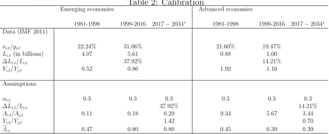
In our calibration exercise, we split the period 1981-2016 into two subperiods of 18 annual observations as 1998 marks the start of a sharp and durable increase in the saving rate of the group of emerging economies. Table 2 shows the data and the assumptions made. We use the average gross national saving in percentage of GDP for both groups of countries over both subperiods in Equation (23) to estimate the values for βA and βB. We rename these estimates as βEE ≡ βA and βAE ≡ βB (where AE and EE respectively stand for advanced and emerging and developing economies). Following the same approach, we use average values for GDP in PPP and population levels to estimate the current account balance of emerging countries in Equation (25) and rename them accordingly. The unknown population levels at the future subperiod which are needed in the calculation of the current account balance during the second subperiod are computed assuming the same growth rate as between the first and the second subperiod. The capital share in output α is assumed to be the same for both groups and to be equal to 0.3.
Before examining the performance of the calibrated model, it is important to emphasize the possible results of an increase in the average propensity to save in the emerging and developing countries. In each of these countries, the additional saving could finance domestic investment, investment in other emerging economies or investment in advanced countries. The “saving glut” hypothesis assumes that a large part of this additional saving is used to buy assets in advanced economies which is reflected in the size of the global imbalances between developed and developing countries. This is precisely this hypothesis we want to test in this calibrated model. Using data on saving, we can run the model to calculate the quantitative effect of the actual increase in the average propensity to save on the current account balance. The figure we obtain for the current account balance per unit of GDP is necessary the aggregate result of four dynamic forces at work in our model: the growth of the relative population size, the relative speed of capital accumulation, the growth of the relative efficiency ratio and the international capital mobility.
First, we assign a value for the ratio AAE
AEE such that the calibrated current account balance
of the group of emerging countries in subperiod 1 matches its actual value, i.e. -1.57% of GDP. Although a ratio lower than one can also yield a negative current account balance for emerging countries, we can notice that the calibrated ratio is higher than 1, which is consistent with the fact that this group of countries is less developed than the group of
Table 2: Calibration
Emerging economies Advanced economies
1981-1998 1999-2016 2017 − 2034∗ 1981-1998 1999-2016 2017 − 2034∗ Data (IMF 2011)
si,t/yi,t 22.24% 31.06% 21.60% 19.47%
Li,t(in billions) 4.07 5.61 0.88 1.00
∆Li,t/Li,t 37.92% 14.21% Yi,t/Yj,t 0.52 0.86 1.92 1.16 Assumptions αi,t 0.3 0.3 0.3 0.3 0.3 0.3 ∆Li,t/Li,t 37.92% 14.21% Ai,t/Aj,t 0.11 0.18 0.29 9.34 5.67 3.44 Yi,t/Yj,t 1.42 0.70 b βi,t 0.47 0.80 0.80 0.45 0.39 0.39
* All the values in the column 2017-2034 are assumed to be same for all subsequent periods.
advanced economies. The objective is then to assess the performance of the model for the second subperiod when we use the actual values for L and Y and the estimated β of both groups in subperiod 2 (1999-2016). We estimate the value of gEE,2
yEE,2, assuming that
the variation in the ratio AAE
AEE is equal to the growth rate of the relative income between
1999 and 2016, and compare it to the actual value of the current account balance of the group of emerging countries. The calibrated model yields a positive current account balance for the emerging countries, which means that condition (18) is satisfied. However, the model slightly underestimates the magnitude of the surplus as it predicts a current account balance per GDP of 1.87% instead of an actual value of 2.36% (Table 3). Despite its simplicity and the strong assumption of perfect capital mobility, this calibrated model rightly predicts the sign of the current account balance actually observed and stresses the effect of an increase in the average propensity to save in the group of emerging economies. Even though it tends to underestimate the magnitude of the current account balance, the performance of this model gives credit to the “saving glut” hypothesis.
Our last exercise consists in running the model in order to see whether global imbalances will keep on increasing or disappear in the next period (2017-2034). We assume that the saving rates, population growth rates and income growth rates remain the same as for the period 1998-2016. The evolution of the efficiency ratio is assumed to be identical to that of the income ratio. The model predicts that the group of emerging countries will experience an average current account balance of -0.4% of GDP, which implies that global imbalances disappear over this period.
For all our predictions, the results are sensitive to the efficiency ratio AAE
AEE only, as this
is the unique parameter for which we have no real data neither available estimates. The slower the catching-up of the emerging economies in terms of efficiency, the bigger global imbalances in the second and subsequent periods and the more slowly global imbalances will disappear.
Table 3: Calibration results
1981-1998 1999-2016 2017-2034 Prediction IMF data Prediction IMF data Prediction
gi,t/yi,t -1.58% -1.58% 1.87% 2.36% -0.44%
6
Global Imbalances and Welfare Analysis
In section 4 it was shown that a higher βA imposed by country A’s government yields a higher transition income growth rate or a higher steady-state income per worker in both countries. It now remains to find how the welfare of the young and the old generations is modified when βA is increased in the short and the long run. Without loss of generality, we will assume that the population growth rates are equal across countries.
6.1
Short-Run Welfare Analysis
Short-run welfare analysis refers to the first two periods of the economy. Two changes may occur during this timespan: the integration of the capital markets and country A’s government intervention on βA. First, recall that the capital markets of both countries are assumed to integrate between t = 0 and t = 1. (Buiter 1981) shows that, in a two-country model with overlapping generations living for two periods, the welfare of the old generations of both countries born at t = −1 is unaffected by the international capital integration, while the young generation born at t = 0 of the country with the higher (lower) psychological discount factor is raised (reduced). The result is obvious for the old generations as their welfare is determined by the past capital stock per worker. For the young generations, the result depends on the effect on the interest rate of the integration of capital markets. Since the capital stock per worker is higher in the country with the higher psychological discount factor, its interest rate is lower than in the foreign country, and therefore increases when capital markets are integrated. An increase in the interest rate has no effect on the saving decision of the young agents, as their preferences are logarithmic, but it does raise the level of their utility. The opposite is true for the country with the lower psychological discount factor. In that country, the integration of capital markets results in a decrease in the interest rate and yields a lower level of utility for the young generation.
Second, when capital is free to move from one country to another, country A’s government imposes an increase in βA whenever it is required to avoid a current account deficit. The welfare effect of this intervention is established in the following proposition:
Proposition 5 In a two-country model with overlapping generations living for two
peri-ods and with integrated capital markets, the welfare of the old generation of both countries born at t = −1 is unaffected by the increase in βA imposed by country A’s government.
In contrast, the welfare effect on the young generation born at t = 0 in both countries is negative.
Proof: As previously, the welfare of the old generations is determined by the past capital stock per worker and is not affected by a change in βA. For the young generations, the proof is given in the Appendix.
(Buiter 1981) considers the welfare effect on the young and the old generations when the economy moves from autarky to open economy between t = 0 and t = 1. Proposition 5 compares the welfare of the young and the old generations in an open economy without government intervention and in an open economy with government intervention. The result is unambiguous: the welfare of the old generations in both countries is unchanged, while the young generations in both countries are worse off. Before analyzing the welfare effect of country A’s government intervention in the long run, it would be interesting to study the welfare effect on the young and the old generations when the economy moves from autarky to open economy with government intervention between t = 0 and t = 1.
Proposition 6 In a two-country model with overlapping generations living for two
peri-ods, the welfare of the old generations born at t = −1 is unaffected as the economy moves from autarky to an open economy with country A’s government intervention. In contrast, the effect on the welfare of the young generation born at t = 0 in country A is negative while it is ambiguous for country B.
Proof: Proof for Proposition 6 can be easily derived from (Buiter 1981)’s results and Proposition 5.
If we consider that the integration of capital markets and the government intervention of one country occur in the same period (between t = 0 and t = 1), then the welfare effect on the young and old generations that has to be considered relates to Proposition 6. In particular, the government intervention in country A worsens the welfare of the young generation of country B and, thus, can offset the gain of the international integration of capital markets for this generation.
6.2
Long-Run Welfare Analysis
Long-run welfare analysis refers to the steady state. (Buiter 1981) analyzes the case of an economy moving from autarky to integrated capital markets. In this section, we study the welfare effect on the young and old generations in an open two-country economy, in which country A’s government has to intervene at the steady state (case 9 in Table 1) in order to avoid current account deficits. In the standard OLG model, the maximum of welfare is attained when the competitive equilibrium coincides with the golden rule. Whereas this remains true for country B in our model, in country A, the welfare gain from moving closer to the golden rule may be offset by the welfare loss resulting from the modification of the intertemporal consumption allocation imposed by country A’s government increase in βA.
Proposition 7 In a two-country model with overlapping generations living for two
peri-ods and with integrated capital markets, country A’s government intervention may result in an increase in the welfare of country B’s young and old generations at the steady state if and only if the market outcome without government intervention leads to capital under-accumulation. Otherwise, the welfare is unambiguously decreased.
Proof: Country A’s government intervention always results in a higher steady-state capital stock per worker in both countries. As a result, it can only be closer to the golden rule capital stock per worker in country B if the economy experiences under-accumulation of capital without government intervention. If the capital stock per worker is initially higher than the golden rule, it can only move away from the optimum.
Proposition 8 The results of Proposition 7 remain true for country A. However, country
A’s generations undergo a specific welfare loss due to the imposed different intertemporal allocation of consumption. As a consequence, even an outcome closer to the golden rule can coincide with a lower level of welfare.
Proof: See the proof for Proposition 7. In addition, we can show that for a given level of capital stock per capita (˜k), any change in the intertemporal consumption allocation re-sults in a decreased welfare level. The intertemporal utility of the representative consumer in country A when the government intervenes is:
U = ln µ 1 1 + βC AA(1 − α)˜kα ¶ + βAln µ βC 1 + βC α(1 − α)A2 A˜k2α−1 ¶ , (26)
where βA is the discount factor of the representative consumer and βC is the discount factor imposed by the government. Since the utility function is concave, we know that utility attains a maximum under the budget constraint whenever βC = βA. If βC 6= βA, then utility is lower. Hence, for a given capital stock per worker, if the imposed discount factor, βC, is higher than the representative consumer’s preference parameter, βA, the welfare of the generations of country A is decreased.
7
Conclusion
Since the end of the 1990s, the world economy has been characterized by large global im-balances, i.e. a situation in which the fast-growing economies finance the current account deficits of the advanced economies. The purpose of this paper is to build and calibrate a two-country growth model with overlapping generations to investigate the effect of the “global saving glut” ((Bernanke 2005)) on the current account balance of the developed and developing economies. A number of results are obtained. Proposition 1 derives the
conditions for steady-state current account deficits (surplus) when two economies differ in their tastes, in their population growth rates, or both. Proposition 2 gives the condition for an intertemporal equilibrium with global imbalances to exist. Proposition 3 shows that a government’s intervention in the fast-growing economy to avoid current account deficits implies a decrease in the world interest rate, while its effect on the transition growth rate is positive (Proposition 4).
We calibrated this model with averaged IMF data over two periods of 18 annual observa-tions. While the simplicity of the model allows us to make only one assumption regarding parameter values (efficiency ratio AAE
AEE), it correctly predicts the reversal of the current
account balance of emerging countries in the period 1999-2016. In addition, the model predicts that global imbalances will disappear during the period 2017-2034.
Propositions 5 and 6 analyze the welfare effect of both the integration of capital markets and the government’s intervention in the fast-growing country on the young and the old generations. While this effect is null for the old generations in both countries, it is negative for the young generation of the fast-growing economy and is ambiguous for the young generation of the slow-growing economy. In the long run, the effect of the government’s intervention in the fast-growing country on the welfare of the young and the old generations in the slow-growing country may be positive if there is under-accumulation of capital and is negative otherwise (Proposition 7). The welfare effect on the young and the old generations of the fast-growing country is more complicated as the government of this country modifies their choice of intertemporal allocation of income. Proposition 8 shows that this welfare effect is negative.
This framework with perfect capital markets can be extended in a number of ways. For instance, the model is flexible enough to add capital market imperfections in order to study the relationship between global imbalances and imperfections in the capital markets in slow-growing economies. Another interesting line of research would be a framework in which purchasing power parity does not hold and in which exchange rates are subject to manipulation.
References
Bernanke, Ben. 2005. “The Global Saving Glut and the U.S. Current Account Deficit.” Sandridge Lecture, Virginia Association of Economics, Richmond, VA (March 10). Bernanke, Ben S. 2007. “Global Imbalances: Recent Developments and Prospects.”
Speech at the Bundesbank Lecture, Bundesbank, Berlin (September 11).
. 2009. “Financial Reform to Address Systemic Risk.” Speech at the Council on Foreign Relations, Washington, D.C., (March 10).
BIS. 2009. 79th Annual Report. Chap. 1. Bank for International Settlements.
Blanchard, Olivier J, and Gian Maria Milesi-Ferretti. 2010. “Global Imbalances: In Midstream?” CEPR discussion papers 7693, Centre for Economic Policy Research. Buiter, Willem. 1981. “Time Preference and International Lending and Borrowing in an
Overlapping-Generations Model.” Journal of Political Economy 89:769–795.
Caballero, Ricardo J., Emmanuel Farhi, and Pierre-Olivier Gourinchas. 2008. “An Equi-librium Model of ”Global Imbalances” and Low Interest Rates.” American Economic
Review 98 (1): 358–93.
Desroches, Brigitte, and Michael Francis. 2010. “World real interest rates: a global savings and investment perspective.” Applied Economics 42 (22): 2801–2816. Higgins, Matthew. 1998. “Demography, National Savings, and International Capital
Flows.” International Economic Review 39 (2): 343–69 (May).
IMF. 2000. “Recovery from the Asian Crisis and the Role of the IMF.” Technical Report, International Monetary Fund, Washington, D.C.
. 2004. World Economic Outlook. Chap. 3. International Monetary Fund. . 2005. World Economic Outlook. Chap. 2. International Monetary Fund. Krugman, Paul. 2007. “Will there be a dollar crisis?” Economic Policy 22 (07): 435–467. Laibson, David, and Johanna Mollerstrom. 2010. “Capital Flows, Consumption Booms and Asset Bubbles: A Behavioural Alternative to the Savings Glut Hypothesis.”
Economic Journal 120 (544): 354–374 (05).
Obstfeld, Maurice, and Kenneth Rogoff. 2007. “The Unsustainable U.S. Current Ac-count Position Revisited.” In G7 Current AcAc-count Imbalances: Sustainability and
Adjustment, NBER Chapters, 339–376. National Bureau of Economic Research, Inc.
. 2009. “Global Imbalances and the Financial Crisis: Products of Common Causes.” CEPR discussion papers 7606, Centre for Economic Policy Research. Portes, Richard. 2009. “Global Imbalances.” In Macroeconomic Stability and Financial
Regulation: Key Issues for the G20, edited by Mathias Dewatripont, Xavier Freixas,
Taylor, John B. 2009, January. “The Financial Crisis and the Policy Responses: An Empirical Analysis of What Went Wrong.” NBER working papers 14631, National Bureau of Economic Research, Inc.
Whelan, Karl. 2010, April. “Global Imbalances and the Financial Crisis.” Working papers 201013, School of Economics, University College Dublin.
8
Appendix
To prove that the welfare effect of country A’s government intervention on country A’s young generation born at t = 0 is negative (Proposition 5), it suffices to study the differ-ence between the utility U0 of the young generation resulting from the market outcome,
and the utility UC
0 resulting from any other imposed psychological discount factor βC, ceteris paribus. This difference can be expressed as:
D(βC) = U0− U0C = ln µ 1 1 + βA AA(1 − α)kαA,0 ¶ + βAln µ βA 1 + βA AA(1 − α)kαA,0AAαkα−1A,1 ¶ −ln µ 1 1 + βC AA(1 − α)kA,0α ¶ − βAln µ βC 1 + βC AA(1 − α)kαA,0AAαkα−1C,1 ¶ ,(27)
where D(βC) is the difference between the utilities of the young generation without and with government intervention, and kC,1 the per capita stock of capital in country A at
t = 1 under the optimization based on βC instead of βA. We can rewrite Equation (27) as:
D(βC) = ln µ 1 + βC 1 + βA ¶ + βAln à βA 1 + βA 1 + βC βC kα−1 A,1 kα−1 C,1 ! = ln(1 + βC) − ln(1 + βA) + βAln µ βA 1 + βA ¶ + βAln(1 + βC) − βAln(βC) + βA(α − 1)ln µ kA,1 kC,1 ¶ . (28)
We know from Equations (10) that:
kA,1 kC,1 = LA,0 βA 1+βAAAk α A,0+ LB,01+ββBBABkB,0α LA,01+ββCCAAkA,0α + LB,01+ββBBABkB,0α . (29) Hence, D(βC) = ln(1 + βC) − ln(1 + βA) + βAln ³ βA 1+βA ´ + βAln(1 + βC) − βAln(βC) −βA(1 − α)ln ³ LA,01+ββAAAAkA,0α + LB,01+ββBBABkB,0α ´ +βA(1 − α)ln ³ LA,01+ββCCAAkαA,0+ LB,01+ββBBABkαB,0 ´ . (30)
If βC = βA, then D(βC) = 0. Whenever it is required, country A’s government interven-tion results in a higher preference parameter than that of the representative consumer. Therefore, we merely have to compute the first derivative of D(βC) with respect to βC and observe its sign when βC > βA. The derivative of D(βC) with respect to βC is:
∂D ∂βC (βC) = βC − βA βC(1 + βC) + βA(1 − α)LA,0AAk α A,0 (1 + βC)2 ³ LA,01+ββCCAAkαA,0+ LB,01+ββBBABkαB,0 ´. (31)
If βC > βA, Equation (31) is positive. Therefore, the utility of country A’s young genera-tion born at t = 0 diminishes when its government has to intervene (cases 7, 8 and 9) in order to avoid a current account deficit. We can conclude that the welfare of country A’s young generation is lower in an open economy with countryA’s government intervention than in an open economy without government intervention.
Let us now turn to the welfare effect of country A’s government intervention on country
B’s young generation born at t = 0. Proposition 5 states that the welfare effect is also
negative. The welfare of country B’s young generation born at t = 0 is only affected through the modification of the world interest rate at t = 1. The saving decision of this young generation is unaffected by the modification of βA but its consumption in the next period is influenced by the world interest rate at t = 1. An increase in βA results in more saving in country A leading to a lower world interest rate at t = 1. This lower interest rate decreases the consumption of country B’s young generation (born at t = 0) at t = 1 while leaving unchanged its consumption level at t = 0 due to the logarithmic form of the utility function. In total, the welfare of this young generation decreases. Consequently, any increase in βA results in a decrease in the welfare of the young generation at t = 0 in country B.
![Figure 2: Gross national saving and investment as a percentage of GDP (1981-2016) [Logarithmic scale; (S): saving and (I): investment]](https://thumb-eu.123doks.com/thumbv2/123doknet/6024919.150624/6.892.176.766.126.558/figure-gross-national-saving-investment-percentage-logarithmic-investment.webp)