Experimental methodologies to explore 3D development of biofilms in porous media

En vue de l'obtention du

DOCTORAT DE L'UNIVERSITÉ DE TOULOUSE

Délivré par :

Institut National Polytechnique de Toulouse (Toulouse INP)

Discipline ou spécialité :

Dynamique des fluides

Présentée et soutenue par :

Mme ANNE LARUE

le mardi 27 mars 2018

Titre :

Unité de recherche :

Ecole doctorale :

Méthodologies expérimentales pour l'étude du développement 3D de

biofilms en milieux poreux

Mécanique, Energétique, Génie civil, Procédés (MEGeP)

Institut de Mécanique des Fluides de Toulouse (I.M.F.T.)

Directeur(s) de Thèse :

M. YOHAN DAVIT

Rapporteurs :

M. FABRICE GOLFIER, UNIVERSITÉ LORRAINE M. LAURENT OXARANGO, UNIVERSITE GRENOBLE ALPES

Membre(s) du jury :

M. ETIENNE PAUL, INSA TOULOUSE, Président

Mme SABINE ROLLAND DU ROSCOAT, UNIVERSITE GRENOBLE ALPES, Membre M. PASCAL SWIDER, INP TOULOUSE, Membre

Acknowledgements

First and foremost, I am extremely grateful to my thesis supervisors Professor Pascal Swider and Doctor Yohan Davit for giving me the opportunity of doing this PhD. Thank you for trusting me in carrying out this project and for believing in my abilities. I particularly appreciated the autonomy you granted me for this work which enabled me to express my ideas and to remarkably improve my capacities. Thank you for your precious advice, guidance and encouragements throughout these years.

I would like to thank Professor Laurent Oxarango and Doctor Fabrice Golfier for metic-ulously examining my work and for their interesting remarks and comments which helped in the preparation of my defence. I am also grateful to the other members of the jury, Professor Etienne Paul and Doctor Sabine Rolland du Roscoat for their reviews and suggestions.

Very special thanks to CNRS research director Michel Quintard for overseeing my progress over the years and for his helpful critics and remarks which improved the quality of my work. I am as well sincerely grateful to Doctor Paul Duru for his guidance and advice on X-ray imaging and experimental aspects.

I wish to address very warm thanks to Doctor Sophie Allart and Danièle Daviaud for their collaboration to my work at the imaging facility of the Centre de Physiopathologies de Toulouse Purpan. Thank you for all the time you poured into assisting me with my experiments, developing new ideas and for your thorough help and support. I also thank Astrid Canivet and Magda Rodrigues for their assistance.

I am particularly indebted to Ruddy Soeparno for his collaboration to my experimental work. It was a privilege to work with you. Thank you so much for the time and care you invested in my experimental workbench and for your help, availability, advice as well as encouragements in the difficult moments. I also wish to thank Jérôme Briot for his ingenious ideas which brought my protocols to a greater level of sophistication, thank you additionally for your availability and support. I am as well grateful to Maëlle Ogier for her help and guidance throughout the various stages of my thesis. A special thanks to Benjamin Duployer for his assistance on X-ray imaging.

I would like to express my sincere gratitude to CNRS research director Sylvie Lorthois, Doctor Pauline Assemat and Professor Manuel Marcoux for their encouragements and interest in my work during those three and a half years.

A heartfelt thanks to my friends and colleagues of IMFT who brought their warmth, laughs and encouragements every single time, especially Amy, Vincent, Maxime, Baptiste and Roxanne. A particularly warm thanks to Adlan for our existential musings and Yara

for our long and desperate talks! Thank you both for sharing your good humour and you experimental traumatic experiences which boosted my spirits! Thank you Myriam for our musical sessions and talks which relaxed daily stresses.

A very warm thank you to my long-time friends Morgane, Sandra, Pauline, Mélanie, Juliette, Youssouf, Ulysse for you support, laughs and positiveness which kept me from going crazy (or has it?). To my karate sensei and friends who patiently and martially coped with my stressful days. To my bouldering friends, Manon and Jean-Marc, for these special exhausting evenings of stress relief. To all my friends who encouraged me, cheered me up regularly and believed in me, Xavier, Marie and Thierry, Nanda and Didier. Special acknowledgements to Béatrix de Warren for the work together which was of tremendous help.

I also have a cute thought for my cat, Shadow, whose soothing purr accompanied my long writing nights.

A profound thank you to my family for their constant love and support. To my late brother and father, I am sure you would have been very proud of me.

Finally, I would like to thank the most important person in my life, Alix. None of this would have been possible without you by my side. Thank you for your unconditional love and support during those years. This thesis is dedicated to you.

Contents

3

5 General introduction

I Exploring microbial growth in porous media 1

The world of biofilms 7

1.1 Ubiquity of biofilms in our environment . . . 7

1.2 First insights into microbiology . . . . 8

1.2.1 Bacterial generalities . . . . 8

1.2.2 Appendages . . . . 9

1.2.3 Overview of metabolism . . . . 10

1.2.4 Reproduction . . . . 11

1.3 Bacterial biofilms . . . 11

1.3.1 Development stages of a biofilm . . . 12

1.3.2 Biofilm morphology with respect to environmental constraints . . . 14

2 Biofilms in porous media 17 2.1 Biofilms in natural and industrial porous media . . . 17

2.1.1 Insights on porous media . . . . 17

2.1.2 Stream-aquifers biofilms . . . 19

2.1.3 CO2 capture and sequestration (CCS) . . . . 20

21 2.2 Porous media: the biofilms and hydrodynamics playground . . . 2.3 Inquiry about the need of experimental methods to assess the influence of 25 hydrodynamics on biofilms . . . 3 Imaging of Biofilms 27 3.1 State of the art of biofilm imaging techniques . . . 27

3.1.1 Imaging of biofilms on flat substrates or 2D porous media . . . 27

3.1.2 3D imaging of biofilm in opaque porous substrates . . . 32

3.2 Investigating the potential of X-ray micro-tomography . . . . 33

3.2.1 Insights into X-rays generation . . . . 33

3.2.2 X-ray interaction with materials . . . 35

3.2.3 Creating a 3D image X-ray micro-tomography image . . . . 37

3.2.4 Employing X-rays to image biofilms in porous media . . . 39

3.3 Inquiry regarding the need of protocols for biofilm observation in porous media 45 4 Thesis Purview 47 II Proposal of a biofilm imaging protocol using X-ray micro-tomography 51 5 Introduction 53 6 Materials and Methods 55 6.1 Contrast agent preparation . . . . 55

6.2 Biofilm growth protocol . . . 56

6.2.1 Strain preparation and capillary inoculation . . . . 56

6.2.2 Fluidic experimental set up . . . . 57

6.3 Imaging protocol . . . . 58

6.3.1 Two-photon microscopy (TPLSM) . . . . 58

6.3.2 X-ray micro-tomography (X-ray CMT) . . . 61

6.4 Uncertainty measurement . . . . 62

6.5 Image processing . . . . 62

6.5.1 TPLSM acquisition . . . . 63

6.6 Segmentation for both imaging modalities . . . . 64

6.7 Metric analysis . . . . 65

7 Results of our protocol 67 7.1 Viscosity measurements . . . . 67

7.2 Bead phantom uncertainty analysis . . . . 68

7.3 Comparison of TPLSM and X-ray CMT acquisitions . . . . 70

8 Discussion 77 8.1 Uncertainty analysis . . . . 77

8.2 Comparing two-photon microscopic images with X-ray micro-tomography images 77 79 81 83 9 Conclusion III Design of an experimental workbench for the characterisation of biofilms in porous media under controlled growth conditions 10 Introduction 11 Description of the experimental workbench 85 11.1 The fluidic circuit . . . 85

11.1.1 General description . . . . 85

11.1.2 The micro-fluidic pressure controller . . . 87

11.1.3 The ultra-pure water reservoirs . . . . 90

11.1.4 Syringe pumps . . . . 91

11.1.5 Differential pressure sensors . . . 92

11.1.6 Dissolved oxygen sensors . . . . 93

11.1.7 Online spectrophotometer . . . . 93

11.2.1 The porous media . . . . 94

11.2.2 Controlling hydrodynamics parameters . . . . 96

11.2.3 Permeability measurements . . . . 97

11.2.4 Dissolved oxygen measurements . . . . 98

100 11.2.5 Controlling bioreactor inoculation . . . . 12 Performance of the system 101 12.1 Univariate analysis of monitored variables . . . . 101

12.1.1 Methods used to obtain global trend . . . . 101

12.2 Differential pressure curves . . . 102

12.2.1 Deriving permeability from differential pressure curves . . . 104

12.3 Temperature curves . . . . 105

12.4 Dissolved oxygen curves . . . . 105

12.5 Control curves at 1 ml/min . . . . 107

12.6 Absorption measurements . . . . 110

110 12.7 Conclusion . . . . 13 Versatility of the system 113 13.1 Experimental perspectives . . . . 113

13.1.1 Changing the bio-chemical conditions . . . . 113

13.1.2 Customized hydrodynamical conditions . . . . 114

13.1.3 Adaptation to diverse porous media . . . . 114

13.2 Limitations of the system . . . . 115

13.2.1 Technical limitations . . . . 115

13.2.2 Difficulties encountered . . . 115 116 13.2.3 Proposed technical improvements . . . .

IV Example application: Investigating the effects of flow velocity on the

temporal development of P. aeruginosa biofilm in porous media. 121

15 Introduction 123

16 Materials and Methods 125

16.1 Biofilm growth protocol . . . 125

16.1.1 Degassing the bioreactor . . . . 125

16.1.2 Strain preparation and bioreactor inoculation . . . . 125

16.1.3 Preparation of fluidic circuit . . . 126

16.2 Imaging protocol and processing . . . . 128

16.2.1 Contrast agent injection . . . . 128

16.2.2 Acquisition set up and parameters . . . . 128

16.2.3 Image processing . . . . 129

17 Results and discussion 131 17.1 Analysing monitored variables . . . . 131

17.1.1 Experiment at 0.5 ml/min . . . . 131

17.1.2 Experiment at 1 ml/min . . . . 134

17.1.3 Experiments at 2 ml/min . . . . 136

17.2 Difference between flow rates . . . 138

17.3 Images analysis . . . . 142

151

155 General conclusion

Perspectives

A Chapter II complementary experiments and image processing 157

A.1 Measuring the density of MicroOpaque BaSO4 suspension . . . . 157

A.2 Contrast agent rheology . . . . 158

A.3 Determining culture media concentration inhibiting bacterial development . . 161

A.4 Point spread function reduction trials . . . . 163

A.5 Bright-field microscopy control measurements . . . 166

167 A.6 Filling hollow biofilm structures from TPLSM images . . . B Chapter III complementary experiments and image processing 171 B.1 3D-printed parts detailed plans . . . . 171

B.2 Design plans for bioreactor . . . . 175

B.3 Darcy equations for permeability . . . . 177

B.4 Residual curves . . . . 178

B.5 Permeability from raw data . . . . 180

B.6 Filtering raw oxygen data . . . . 181

183 B.7 Additional control curves at 1 ml/min . . . . C Chapter IV complementary experiments and image processing 185 C.1 Oscillating flow paths in preliminary experiments . . . 185

C.2 Permeability curves from raw measurements . . . . 187 188 C.3 Flow curves . . . .

List of Figures

1.1 Left: epifluorescence microscopic image of a poly-microbial biofilm grown on a stainless steel surface in a laboratory potable water biofilm reactor [64] and right: scanning electron micrograph of a staphylococcal biofilm on the inner surface of an indwelling medical device [64] (scale bars 20 µm). . . 7

1.2 Proteus vulgaris flagella and fimbriae. Image from Prescott’s Microbiology [233] 9

1.3 Conceptual drawing of biofilm formation and maturation from Hall-Stoodley & Stoodley, 2002 [88]. . . 13

1.4 Biofilm morphology under high shear rates (left) and low shear rates (right) [89]. Other filamentous bacteria and archeal biofilm occur in hot springs, ma-rine hydrothermal vents and acid mine drainage runoff [169] . . . 15

2.1 Various hierarchically structured natural porous media [108]. . . 18

2.2 Microbial ecology in the streambed [18]. . . 19

2.3 Conceptual illustration of a biofilm barrier in super-critical CO2 storage [150]. 21 2.4 Matrix-producing P. Aeruginosa appears in green and non-producing mutant is

in red. A: flow paths were visualised by flowing multiple beads in the chamber, it could be seen that regions occluded from flow allow non-matrix-producing mutants to develop. B and C show the difference of co-existence of these competitive strains in simple flow and a porous medium [154].. . . 22

2.5 Oscillating pressure drop over growth period (left) and influence of sucrose on maximum pressure drop (right) observed by Stewart et al [193]. . . 24

3.1 Left: AFM view of a 3-week old biofilm of a sulfate-reducing bacterium of genus Desulfrovibrio [19], the cells are seen to form a close aggregate. Right: SEM image of the surface of a mixed species (Staphylococcus Epidermidis and

Klebsiella oxytoca) biofilm on a 63-day old catheter [79]. Scale bars: 5µm. . . 28

3.2 Left: basil pistil and pollen grains fluorescing in green after excitation with a neon white light. Right: biofilm image by two-photon microscopy where the bacteria expressed green fluorescent protein (GFP) and a red fluorophore (tetramethylrhodamine linked to Concanavalin-A) marked certain polymers of the EPS matrix. . . 29

3.3 Principle of fluorescence microscopy: the source sends the laser at a certain wavelength to excite the focal plane, the signal from the specimen is filtered back. Source: Centre de Physiopathologies de Toulouse Purpan. . . 30

3.4 Left: 12-day old stream biofilm forming quasi-hexagonal structures [17]. Right: biofilm attached to the surface of glass beads after 60h of growth under constant flow rate [122]. . . 31

3.5 Time-resolved biofilm deformation observed by optical coherence tomography [23]. . . 31

3.6 Biofilm in porous media images by magnetic resonance microscopy [178]. The first column (T2) maps the of proportion fluid phase (white-yellow colour cor-responding to mobile free water) and biomass (red-orange colour corcor-responding to less mobile water in the biofilm). The third column illustrates the veloc-ity maps for an average tube velocveloc-ity of 1.42 mm/s. Spatial resolution is 54.7 µm/pixel over 1000 µm for velocity and 200 µm for T2. Corresponding histograms are also shown in columns two and four respectively.. . . 33

3.7 Left: synchrotron image (EPSIM 3D/JF Santarelli, Synchrotron Soleil). Right: image of a storage ring by European Synchrotron Radiation Facility (ESRF), both in France. . . 34

3.8 Typical tomography set up [231] where generated X-rays pass through the sample and the attenuated rays are perceived by the detector.. . . 35

3.9 The different electron shells. Image from The Essential Physics of Medical Imaging [32]. . . 35

3.10 X-ray attenuation as a function of energy for some elements used in [7], namely Barium, soil and rock samples, Iodine, water and 1:6 mixture of water and KI. It can be observed that all elements except water have absorption edges, illustrated by the sharp discontinuity in the attenuation curve. . . 36

3.11 X-ray CMT common artefacts: beam hardening (left) which can be observed as the difference in gray level of the same material near the sample’s edge [231] and ring artefacts (right) appearing as concentric circles on the cross section of a superconductor strand [26]. White dashed circles were added to aid visualisation. . . 38

3.12 Potentially available contrast agents, enhancing the contrast of a specific phase or interface in a biofilm-water sample. Iodide solutions and Iron(II) sulfate mark the biofilm phase, barium sulfate and 1-chloronaphtalene mark the aque-ous phase and silver microspheres enhance the water/biofilm interface. Biofilm image obtained by two-photon microscopy.. . . 40

3.13 Images of biofilm in 2D porous media by shadowscopy (left) and X-ray radio-graphy (centre). Region of different colour map were chosen for comparison. Right: 3D image of biofilm (purple) in porous media (gold) using X-ray micro-tomography [58]. . . 41

3.14 Left: images of biofilm in 2D porous media by light microscopy (top) and X-ray CMT (bottom). Right: 3D image of biofilm (green) in porous media (gold) using X-ray micro-tomography [106]. . . 42

3.15 Images of the sample with 1-chloronaphtalene (left) and precipitated barium sulfate (right). Images from Roscoatet al. 2013 [174] . . . 43

3.16 (A) biofilm column imaged in phase contrast with biofilm marked with F eSO4 and (B) in absorption contrast (right) with the fluid marked with BaSO4. On the right corresponding segmentation performed for volume analysis. The centre image represents the grey level histograms of (A) and (B) [33]. . . 44

6.1 Fluidic circuit with which biofilm was grown for 2 days at fixed flow rate. . . 58

6.2 Set up for TPLSM imaging: the black thermostated cubicle enclosed the sample and lens (see zoomed section where the immersion lens can be observed), a green syringe pump maintained flow in the sample to prevent excess heating of the sample due the laser. . . 59

6.3 3D printed capillary holder with silicone filled plugs and integrated pool for immersion lens. The four notches enable 4 different angles. The sketch on the right illustrates the capillary’s position with reference to the lens. . . 60

6.4 Biofilm structure obtained on first (0°) and fourth (360°) acquisition. Fractures can be observed on the 360° image, showing the effect of a high power laser on the biofilm. . . 61

6.5 From left to right: the image acquired with the flow cell positioned at 0° (a & d), then the image acquired with the flow cell rotated at 90° (b & e), where the complementary information on the biofilm grown on the top and bottom walls can be observed. At the far right (c and f) are the merged stacks of a & b and d & e respectively.. . . 64

6.6 X-ray absorbent micro-spheres (turquoise arrows) in contrast agent and barium sulfate aggregates (violet arrows). The scale bar indicates the size difference enabling the distinction between them. . . 65

7.1 Left: the shear stress of three samples of contrast agent (in blue) plotted against shear rate ˙γ = [1, 3, 10, 30, 100, 300]s−1 at 37℃. Undiluted barium sul-fate suspension was used as control and measured at ˙γ = [10, 20, 100]s−1 at 37℃. Right: the viscosity of three samples of contrast agent (in blue) plotted against shear rate. Pure barium sulfate suspension (in red) can be seen to be more viscous. . . 67

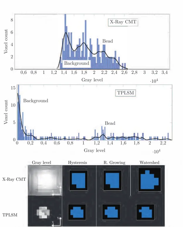
7.2 Top and middle: gray level histograms of a bead imaged by X-ray CMT and TPLSM respectively. The smoothing spline (black) illustrates the main peaks. For X-ray CMT, the first two left peaks belong to the greyish background, the last one represents the bead. For TPLSM, the left peak belongs to the black background and the small centre peak represents the bead. Bottom: gray level images of a bead via X-ray CMT and TPLSM along with the results of the three segmentation techniques namely hysteresis, region growing and watershed. TPLSM spatial resolution was 1.186 µm/pixel (5 pixels ∼ 6 µm) and X-ray CMT was 2 µm/pixel (3 pixels= 6 µm). . . 69

7.3 Top: mean phantom diameter determined in X, Y and Z directions and equiv-alent spherical diameter derived from 3D volumes, the error bars representing the standard deviation. Measurements were made by processing the same beads with different segmentation techniques namely region growing, watershed and hysteresis. Bottom: mean surface area (left) and mean volume (right) are illustrated. For all plots, the control dimensions (supplier information and bright-field microscopy) are also illustrated. . . 70

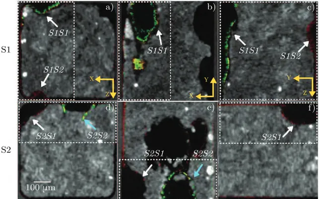
7.4 Visual comparison of TPLSM images superimposed on X-ray CMT stacks for two samples (S1 upper and S2 lower). a) and d) illustrate the cross section of the flow cell (XZ) for two different samples, b) & e) and c) & f) show the side view XY and YZ respectively. White dashed rectangles represent the portion of the flow cell used for quantitative analysis, the arrows show TPLSM structures appearing hollow (white) and whose contour are not well-delineated (cyan). . 72

7.5 On the left, TPLSM binary image with hollow structure and on the right, the TPLSM* image with void spaces filled. It can be observed that the structure’s contour is untouched. . . 72

7.6 Quantitative analysis of biofilm metrics: volume in upper plot, 3D surface area in middle plot and maximum thickness in lower plot. Each color represents a sample and the three used segmentation are illustrated by different shapes. . 74

7.7 3D visualizations of the analyzed samples showing corresponding biofilm for-mation on the flow cell wall. The different structures are pointed by arrows are are recognizable. . . 75

11.1 Fluidic circuit for biofilm growth using a pressure controller and a flow sen-sor. The bioreactor is the centrepiece of the set up with its embedded porous medium, various sensor inlets and UVC targetted region to prevent biofilm from forming just below and above the porous structure.. . . 86

11.2 The complete 3-storey experimental workbench. Every instruments will be detailed further. Black curtain are used to cover the set up during experiments for protection against dangerous UVC rays. . . 88

11.3 Actual experimental workbench. Every detailed device will be later referenced in this figure. . . 89

11.4 The micro-fluidic pressure controller with 4 available channels and a flow sensor connected to channel 4 on top. . . 90

11.5 The custom-designed large ultra-pure water reservoirs with a immersed UVC lamp, O2 bubbling and constant stirring. . . 91 11.6 The four NEmesys low pressure syringe pumps positioned vertically to protect

the device from eventual leaks and to ease removal of bubbles when refilling the syringes. Two glass syringes with required tubing are also illustrated. . . 92

11.7 Fibre optic oxygen micro-sensors mounted on plastic a plastic syringe. The fibre size was 140 µm. . . 93

11.8 Left: empty bioreactor (front view) and right: bioreactor with embedded porous media (turned ∼ 30°). Every inlets and probing points are shown and the structures was rendered transparent for visual purposes. The characteris-tics are detailed in the following paragraphs. . . 95

11.9 Left: actual bioreactor (front view) with glued quartz slides and right: actual bioreactor turned ∼ 120° bioreactor. Visible inlets and probing points are shown. . . 95

11.10Illustration of Darcy’s law’s parameters. . . 97

11.11Left: small camera with adjustable holder to visualize the fibre inside the biore-actor, the syringes were removed on the left picture for a better visualization. Right: camera snapshot where the needle tip and fibre can be seen inside the bioreactor through the quartz slide.. . . 99

11.12Rotative device for homogeneous inoculation of bioreactors. . . 100

12.1 The differential pressure measurements (black) for 0.5 ml/min over 36 hours and their smoothed trend by a spline function (red) or a Gaussian kernel (green)103

12.2 Residual versus order curve (left) and variance of residues (right) obtained for a 500 µl/min sample. The residual curve time shows two main phases with highly correlated and regular oscillations. The error variance shows a continuous increase. . . 103

12.3 The permeability curves from the raw data (left) and the smoothing spline (right).. . . 104

12.4 The variation of temperature during the experiment. It can be observed that temperature varied from 25℃ and 27℃. . . 105

12.5 The measured oxygen concentration before (red) and after (blue) the porous structure and their spline estimators (green). It can be observed that the ethanol peaks are excluded from the splines. . . 106

12.6 Left: the differential pressure measurements during this control experiment. The peak at the beginning is an artefact due to manipulation (displacement) of the sensor. Right: The temperature increase of the reservoir ultra-pure water due to UVC disinfection. The temperature is seen to remain stable during the rest of the experiment. . . 107

12.7 Left: the measured oxygen concentration before (red) and after (blue) the porous structure in a non-inoculated bioreactor experiment where a constant decrease of the inlet oxygen concentration can be observed. Right: the perme-ability curve derived from the spline. . . 108

12.8 Measurements of inlet oxygen concentration for four different control experi-ments to assess the influence of UV and O2 bubbling on the effective oxygen concentration reaching the bioreactor. . . 109

12.9 Left: absorbance measurements for an experiment at 0.5 ml/min over 5 hours at the beginning of an experiment, the downward peaks correspond to ethanol hourly cleaning. Right: absorbance measurements over 5 hours at the end of an experiment where the hourly ethanol cleaning is believed to bring biomass from the bioreactor and thus increased absorbance. . . 111

16.1 A 100 µl drop of water and ethanol on a 3D-printed surface. The approximate contact angles clearly demonstrate the hydrophobicity of the polymer as well as its ethanol philicity, the contact angles being > 90 ° and < 90 ° respectively.126

17.1 Left: the differential pressure measurements (black) for 0.5 ml/min over 35 hours and its smoothed trend by a spline function (red) or a Gaussian kernel (green). Right: the first temporal derivative of the spline. . . 132

17.2 Left: the temperature measurements (black) for 0.5 ml/min over 35 hours and its smoothed trend by a spline function (red) or a Gaussian kernel (green). Right: the permeability curve, calculated from the spline. . . 133

17.3 Left: the measured oxygen concentration before (red) and after (blue) the porous structure and their spline estimators (green). It can be observed that the ethanol peaks are excluded from the splines. Right: the oxygen consump-tion curve.. . . 133

17.4 Left: the differential pressure measurements (black) for 0.5 ml/min over 35 hours and its smoothed trend by a spline function (red) or a Gaussian kernel (green). Right: the first temporal derivative of the spline. . . 134

17.5 Left: the temperature measurements (black) for 0.5 ml/min over 35 hours and its smoothed trend by a spline function (red) or a Gaussian kernel (green). Right: the permeability curve, calculated from the spline. . . 135

17.6 Left: the measured oxygen concentration before (red) and after (blue) the porous structure and their spline estimators (green). Right: the oxygen con-sumption curve.. . . 136

17.7 Left: the differential pressure measurements (black) for 0.5 ml/min over 35 hours and its smoothed trend by a spline function (red) or a Gaussian kernel (green). Right: the first temporal derivative of the spline. . . 137

17.8 Left: the temperature measurements (black) for 0.5 ml/min over 35 hours and its smoothed trend by a spline function (red) or a Gaussian kernel (green). Right: the permeability curve, calculated from the spline. . . 137

17.9 Left: the measured oxygen concentration before (red) and after (blue) the porous structure and their spline estimators (green). Right: the oxygen con-sumption curve.. . . 138

17.10Summary graph of the information collected on the influence of flow rate on the development on biofilm during our experiments. For clarity purposes, only the splines were plotted. The different ∆P slopes are displayed as well as the amplitude of fluctuations and the maximum differential pressure reached. . . 140

17.11Summary graph of the three permeability curves. . . 141

17.123D visualisation of a) porous medium and biofilm, b) biofilm only, c) porous medium and flow paths (enhanced by contrast agent) and d) flow paths only. 143

17.13Comparison of the spatial distribution of biomass at two different flow rates namely 0.5 ml/min and 1 ml/min. . . 144

17.143D visualisation of bubbles only inside the porous medium of the 0.5ml/min experiment, after segmentation. Their exact position along with their size and volume can be measured from the images. . . 145

A.1 The fluid sample is positioned between the cone and the plane. As an angular velocity is applied to the cone, the plane remains fixed, shearing the fluid. . . 158

A.2 Graph of percentage transmission of the inoculated concentration media.. . . 162

A.3 From left to right: image in the focal plane (XY) with resolution 0.83 µm/pixel, image of the cross-section (XZ) highly distorted due to the point spread func-tion with resolufunc-tion 4.187 µm/pixel, image of the side (YZ) also distorted because of the poor resolution in Z.. . . 163

A.4 Left: original image in grays, right: deconvolved image using Huygens software. A slight improvement is observed but not enough for a reliable segmentation and comparison with X-ray tomographic images. . . 164

A.5 Biofilm grown with sub-resolution blue fluorescent beads. a) Biofilm, b) em-bedded blue beads (brightness was increased to enable a better visualisation). c) beads deformed by point spread function. . . 164

A.6 PTFE and glass flow cells with biofilm. Images of focal plane (XY) and cross section (XZ). . . 165

A.7 Image of the beads obtained with bright-field microscopy in grey levels (left) and processed and binarized image (right). Visual observation confirm the accuracy of the processing and binarization. . . 166

A.8 3D biofilm structure in turquoise, formed on the capillary corner. Original signal has a rough surface as shown with the arrow indicating thin biofilm structure on the capillary wall. Restored signal is smooth and signal under reconstruction is red as shown by the top arrow. The contour of the void structure on the capillary wall is drawn in black. The signal from inside the corner corresponds to the contour of the biofilms structure. . . 167

A.9 3D biofilm structure in turquoise on upper left images and orthogonal views on the other screens. Bottom left image shown straing line being drain from the furthest perceived signal. This is done on several slices and it can be seen on the other views that the part under restored corresponds to the capillary corner. . . 168

A.10 Void structure being filled, interpolation result displayed on upper right image. Orthogonal views confirm that no extra signal is being inserted. Upper left image shows 3D image of structure.. . . 169

B.1 3D printed holders for sensors, bioreactor and camera. All of them can slide in the Norcan shaving ’rail’ and be held in place with the fixable gib.. . . 171

B.2 Top, front and section views of the fixable slider, bioreactor holder and flow sensor holder. . . 172

B.3 Top, front and section views of the pressure sensor holder and front and side views of the syringe-mounted optode holder.. . . 173

B.4 Camera positioning devices parts: the camera holders for the top and bottom optodes which fit and rotate in the trunk, itself fitting and rotating within the base. . . 174

B.5 Front and side main views of the bioreactor, their respective cross-section views are named by a letter and represented by a line crossing the main front or side view. . . 176

B.6 Residual versus order and residual versus fitted curves. . . 178

B.7 The two phases of the residual versus order curves. The data seems highly correlated. . . 178

B.8 The two phases of the residual versus fitted curves. The data seems highly correlated. . . 179

B.9 The thresholded values of differential pressure and the un-thresholded perme-ability curve. . . 180

B.10 The filtered values for oxygen measurements. The selected values for the spline are in green. Top left: sample at 0.5 ml/min, top right sample at 1 ml/min and bottom sample at 2 ml/min. . . 181

B.11 Filtering the low frequencies in Fourier . . . 182

B.12 Choosing a modulus band in Fourier . . . 182

B.13 Differential pressure curves for an O2 bubbled reservoir with UV (left) and without UV (right). . . 183

B.14 Differential pressure curves for a non-bubbled reservoir with UV (left) and without UV (right). . . 184

C.1 Overlaid pressure curves for the experiments at 1 ml/min (left) and 2 ml/min (right).. . . 185

C.2 Flow paths image for the experiments at 1 ml/min . . . 186

C.4 Raw permeability curves for the experiments at 1 ml/min (left) and 2 ml/min (right) . . . 187

C.5 Raw flow curves for the experiments at 0.5 ml/min (left) and 1 ml/min (right). 188

List of Tables

7.1 Absolute error, relative and normalized by 6 µm (supplier’s information) and 6.7 µm (bright-field microscopy), for TPLSM and X-ray CMT and using the three segmentation techniques (region growing, hysteresis and watershed). . . 71

7.2 Absolute error, relative and normalized by supplier’s information and bright-field microscopy for 3D metrics (surface area and volume) of TPLSM and X-ray CMT imaged beads. . . 71

12.1 Summary of the influences UV disinfection - through an increase in temperature and decrease in oxygen solubility - and bubbling with oxygen, where decrease in O2 solubility in the main reservoir happened because of a lesser proportion of oxygen and the trapping of bubbles in the bioreactor as DO2 moved back to the gaseous state.. . . 110

17.1 Summary of ∆P slopes characteristics of the different samples. . . . 138

17.2 Summary of important features about the variation in differential pressure for every sample. . . 139

17.3 Biofilm volume and consequent final porosity of the colonised porous medium under two different flow rates namely 0.5 ml/min and 1 ml/min. . . 142

Biofilms are complex microbial colonies developing on interfaces, usually with a liquid phase, where the micro-organisms are nested in a self-secreted polymer matrix. These mi-crobial communities are ubiquitous in our environment and form the slimy matter on rocks at river bottoms, the viscous deposit in water pipes, the plaque on our teeth and the mucus in our lungs. The biofilm mode of growth is well-established in the scientific community and is starting to conquer the general public, replacing the idea of free-floating bacteria. These microbial communities play a crucial role in many environmental processes and their effects vary from desirable, through bothersome, to disastrous, depending on where they are formed and on their microbial specificities [89,134]. For example, desirable effects are the activities of biofilms accumulated in wetlands [167] and in the trickling filters used in wastewater treat-ment plants [22,99] where biofilms remove organics and pollutants from water. Examples of undesirable effects are biofilms accumulated in cooling towers or other heat exchangers where they increase heat transfer resistance [134], they can also be responsible for the contamination of water distribution pipelines [132, 213]. Finally, biofilms having disastrous effects are the ones developing on implantable prosthetic devices where they can cause serious illnesses to the death of the infected patients [81,134,198].

Biofilm formation begins when microorganisms attach to a surface under suitable - and usually strain dependent - nutrient and flow conditions. Some substrates are more favourable to microbial attachment which is the case of porous media as they offer a higher surface to volume ratio. Any material, whether biotic or abiotic, which contains a network of fluid-filled voids can be considered as being a porous medium. This is the case of most materials in our environments let it be soil, rock, sand, wood, sponges and even our body (intestines, lungs, capillary networks and bones to name a few). Many engineering applications are dependent on processes involving the growth of biofilms in porous media, notably soil bio-remediation [78,184,216], CO2storage, bio-filters [190], understanding the fate and transport

of nanoparticles in our environment [112], self-healing concrete [114] and microbial enhanced oil recovery [9]. Biofilms developing in porous media alter the porous structure’s mechanical properties by decreasing the pore size and modifying porosity distribution which consequently influence mass and momentum transport. The biofilm colonisation cycle as it spreads and dies through a porous structure has been shown to be strongly dependent on the hydrodynamical conditions. In turn, the presence of the biofilms also influences the flow paths along with mass and momentum transport on which it is dependent for nutrient availability. These various interplays between biofilm colonisation of a porous structure and hydrodynamical growth conditions are still poorly understood, especially the retroactive effect of fluid flow and biomass accumulation. Other aspects are the effects of hydrodynamics on the distribution of microorganisms in the porous medium and the multi-scale nature of many phenomena. For example, how the restriction of flow in a small pore affects global flow or how biofilms develop in heavily polluted environments, are open questions. Research on these fundamental aspects are limited because currently used imaging methods do not enable direct observation of the biofilms 3D architecture inside the porous medium. Also, the multiple parameters involved in these phenomena are complex to experimentally reproduce and monitor.

The main objective of this work is to propose robust and reproducible experimental methodologies for the investigation of biofilms in porous media. An experimental

work-bench under controlled physical and biological conditions is proposed along with a validated 3D imaging protocol based on X-ray micro-tomography using a novel contrast agent combin-ing barium sulfate with agarose gel to quantify the spatial distribution of the biofilm. The present document is divided into four chapter: firstly, we shall present a state-of-the-art of the principal characteristics of biofilm growth in porous media and then narrow our focus on the imaging and experimental aspects. In the second chapter, we will present a complete protocol for 3D imaging of biofilms in porous media using X-ray micro-tomography. In the third chapter, we shall describe the experimental workbench that we have elaborated and the investigations it unlocks. In the last chapter, we present the first results obtained with this workbench as we assessed the effect of flow velocity of the temporal growth of biofilm in a 3D-printed porous structure. At last we shall discuss the contribution of this work and the perspectives it brings for future studies.

Chapter I

Exploring microbial growth in

porous media

1

The world of biofilms

Contents

1.1 Ubiquity of biofilms in our environment . . . . 7 1.2 First insights into microbiology . . . . 8 1.3 Bacterial biofilms . . . 11

1.1 Ubiquity of biofilms in our environment

Many micro-organisms like bacteria, archaea, fungi and some eukaryotic cells like diatoms, have the ability to stick to surfaces and form complex colonies where they are nested in a self-produced polymer matrix [44,46,89]. These micro-niches are termed biofilms and develop at the interface between two phases like air-liquid [189,230] and mostly solid-liquid where they form on any type of natural and artificial surfaces, for example, in soils and aquifers [25,113,

188], on organic substrates like skin [162], our digestive track [142] as well as plants’ roots and leaves [54,221] and in industrial processes (for instance pipelines [132,157] and ship hulls [209,237]) and medical devices like prostheses and catheters [48,79,81].

Figure 1.1: Left: epifluorescence microscopic image of a poly-microbial biofilm grown on a stainless steel surface in a laboratory potable water biofilm reactor [64] and right: scanning electron micrograph of a staphylococcal biofilm on the inner surface of an indwelling medical device [64] (scale bars 20 µm).

These microbial communities play a crucial role in many environmental processes and their effects vary from desirable, through bothersome, to disastrous, depending on where

they are formed and on their microbial specificities [89,134]. For examples, desirable effects are the activities of biofilms accumulated in wetlands [167] and in the trickling filters used in wastewater treatment plants [22, 99] where biofilms remove organics and pollutants from water. Examples of undesirable effects are biofilms accumulated in cooling towers or other heat exchangers where they increase heat transfer resistance [134], they can also be responsible for the contamination of water distribution pipelines [132, 213]. Finally, biofilms having disastrous effects are the ones developing on implantable prosthetic devices where they can cause serious illnesses to the death of the infected patients [81,134,198]. Also, most chronic infections of the human body whether oral, lung, urinary and vaginal, are due to bacterial biofilms [45,90,213].

In the next paragraphs we shall detail several aspects of bacterial biofilms as they are studied in this work. We shall describe some bacterial properties, biofilm development stages and their response to their growth environment. A complete description of bacterium genus is beyond the scope and the following paragraphs are an introduction to several bacteriology features that might improve the understanding of developed research.

1.2 First insights into microbiology

1.2.1 Bacterial generalities

Bacteria are a large domain of prokaryotic organisms (bacteria and archaea), their size vary from 0.14 µm to a maximum of 10 µm. Prokaryote can be spherical (cocci) or rod (bacilli) shaped, spirochaete (spiral) or vibrio (comma) shaped to name a few [187]. They can also form different arrangement: chains, pairs, grape-like clumps, and more. The distinction between bacteria and archaea lies in differences in their structure and genetics whose description is beyond this work. Bacteria can be divided into two major groups based on their response to the Gram-stain procedure. Gram-positive bacteria stain purple, whereas gram-negative bacteria are coloured pink or red. The difference between these two groups is their cell wall structure [203,233]. Gram-positive cell wall consists of a single 20 to 80 nm thick homogeneous layer of peptidoglycan lying outside the plasma membrane. Peptidoglycan is an enormous mesh-like polymer composed of many identical subunits (it contains sugar derivatives and several different amino acids). The gram-negative cell wall is more complex; it has a 2 to 7 nm peptidoglycan layer covered by a 7 to 8 nm thick outer membrane. Because of the thicker peptidoglycan layer, the walls of gram-positive cells are more resistant to osmotic pressure than those of gram-negative bacteria. Also, the gram-positive bacterial cell wall bears a negative charge [63] given by teichoic acids (polymers of glycerol or ribitol joined by phosphate groups). Teichoic acids are not present in gram-negative bacteria, instead, their outer membrane contains LPS - lipopolysaccharides. These are large, complex molecules containing lipids and carbohydrates and which contributes to the negative charge on the bacterial surface. It also has many important functions. For example, it helps stabilise the outer membrane structure and may contribute to bacterial attachment to surfaces and biofilm formation [63,233].

In this thesis, we shall work with a Pseudomonas aeruginosa strain (ATCC® 10145™) which is a gram-negative, rod-shaped bacterium.

1.2.2 Appendages

Many bacteria also have short, fine, hairlike appendages called fimbriae or pili which is different from conjugation or sex pilus. Fimbriae are helically arranged proteins subunits, a cell may be covered with up to 1,000 of fimbriae, which are about 3 to 10 nm in diameter and up to several micrometers long. Many bacteria have about 1-10 sex pili per cell [233] which often are larger than fimbriae and around 9 to 10 nm in diameter. Some types of fimbriae attach bacteria to solid surfaces such as rocks in streams and host tissues. Type IV fimbriae are also responsible for the twitching motility [146,233] that occurs in some bacteria such as Pseudomonas aeruginosa, Neisseria gonorrhoea, and some strains of Escherichia coli. These pili are situated on the bacterial cell poles [146]. Their movement is by short, intermittent motions that can be up to several micrometers in length. Pseudomonas aeruginosa uses its type IV pili to swim against the flow in a fluid flow environment [185]. This is achieved when the bacteria is oriented with the attached pili type IV pointed in the direction opposite to the flow [148, 181]. Pseudomonas aeruginosa then moves upstream along the surface by repeatedly extending and retracting its pili [185]. This upstream motion is a direct reaction to the shear stress near the surface and is not due to chemotaxis [181]. Pili occur on many Gram-negative bacteria and occasionally, on Gram-positive bacteria [143] and contribute to the hydrophobicity of the cell [128].

Most motile bacteria move by use of flagella which are threadlike appendages extending outward from the plasma membrane and cell wall. Bacterial flagella are slender, rigid struc-tures of about 20 nm across to 15 - 20 µm long. Figure 1.2 shows a bacterium with both fimbriae and flagella. Pseudomonas aeruginosa also swims through fluid environments using its flagella, but upstream movement occurs without flagella [185].

Figure 1.2: Proteus vulgaris flagella and fimbriae. Image from Prescott’s Microbiology [233] Bacteria have other external structures to the cell wall that can serve for protection as

well as attachment to surfaces. Indeed, they produce proteinaceous structures that range from monomeric proteins to protein complexes and include the pili and fimbriae. Other produced structures such as glycocalyx, adhesins, and invasins [126] can be used in cell adhe-sion and attachment to solid surfaces [44], including tissue in plant and animal hosts. Some bacteria can be wrapped in glycocalyx, like Pseudomonas aeruginosa and Streptococcus Pneu-moniae. These extra layers confer protection against various external factors like desiccation, as glycocalyx capsules contain large amounts of water but also protect against phagocytes by rendering the bacterium too large to be engulfed [91]. Other protections conferred by pro-teinaceous layers are from viruses, enzymes, toxic materials, ionic and pH fluctuations and osmotic stress [186,233].

1.2.3 Overview of metabolism

Metabolism groups the chemical reactions occurring in the cell and is divided into two ma-jor parts namely catabolism and anabolism. In catabolism, relatively large organic molecules are broken down into smaller ones that can be oxidized to produce energy whereas anabolism uses energy to synthesise large and complex molecules from smaller ones [233]. In catabolism, the energy provided by the energy source is conserved as Adenosine triphosphate (ATP) which is a complex organic chemical that transports energy from one reaction or location in a cell to another [233]. All organisms need carbon, hydrogen, oxygen, and a source of electrons [233]. When bacteria extract electrons, they transfer them to a terminal electron acceptor in a redox reaction which releases energy that can be used to synthesise ATP. Many other macro-molecules needed by microbes are nitrogen, sulphur, phosphorus, potassium, calcium, magnesium and iron. Bacteria express a wide range types of metabolic types [156] and can be classified into specific groups based on their source of energy, carbon and electrons for redox reactions. Autotrophs obtain their carbon from inorganic sources almost solely from CO2

whereas heterotrophs use organic compounds. Light is the energy source of phototrophs and chemotrophs obtain energy from the oxidation of organic or inorganic chemical compounds. When it comes to electron source, lithotrophs use reduced inorganic substances such as H2S,

H2, NH3, and Fe2+, whereas organotrophs extract electrons from reduced organic compounds

[156,236]. Depending on their energy and electron sources, autotrophs and heterotrophs bear a certain prefix, for example photolithoautotrophic bacteria include cyanobacteria as well as purple and green sulphur bacteria. Nitrifying bacteria and iron-oxidizing bacteria are ex-amples of chemolithoautotrophic bacteria and chemoorganoheterotrophic organisms include most pathogens. When the electron acceptor is oxygen, the organism is said to be aerobic. For anaerobic organisms other inorganic compounds, such as nitrate, sulfate or carbon dioxide are employed. Autotrophs CO2 fixation is crucial to life on earth as it provides the organic

matter on which heterotrophs depend.

Some microbes exhibit great flexibility on their metabolic types in response to environ-mental changes, for example many purple non-sulfur bacteria act as photoorganotrophic het-erotrophs in the absence of oxygen but oxidise organic molecules and function chemoorgan-otrophically at normal oxygen levels [233]. Additionally, under nutrient-limiting conditions, many bacteria have developed starvation-survival strategies enabling them to persist in the

environment until conditions become favourable for growth [224]. Most bacterial species form ultra-microcells - less than 0.3 µm - and go in metabolic arrest which allows the organisms to survive for long periods of time when no sufficient energy for growth and reproduction is available [152]. Some bacteria seem able to use almost anything as a carbon source. For exam-ple, Burkholderia cepacia which can employ over 100 different carbon compounds. Bacteria metabolic types are employed to degrade a variety of substances. For instance, actinomycetes which is a common soil bacteria, can break down amyl alcohol, paraffin and even rubber. Several bacterial metabolic reactions are important ecological processes like denitrification and sulfate reduction [41].

Pseudomonas Aeruginosa used in this work is a facultatively anaerobe and a chemoorganoheter-otrophic bacterium.

1.2.4 Reproduction

Prokaryote reproduce by binary fission which is a simple type of cell division. The cell elongates, replicates its chromosome and separates the new DNA molecules to the opposites ends of the cell. A cross wall is then formed in the middle of the elongated parent cell which divides it into two daughter cells. Many prokaryote contain extra-chromosomal DNA molecules called plasmids that are small, double-stranded DNA molecules that can exist independently of the chromosome. Their genes are not essential to their hosts but they usually give the latter a selective advantage in some environments. Plasmids are inherited during cell division, but they are not always equally apportioned into daughter cells and sometimes are lost.

1.3 Bacterial biofilms

Bacteria express two modes of growth namely planktonic state or "free floating" and biofilm state [46, 89]. Based on observation of laboratory and wild bacterial cultures which were covered with a glycocalyx film, John William Costerton proposed the term "biofilm" in 1978 and suggested it was the natural mode of growth of most microorganism [44, 47] especially in systems with high surface area to volume ratios like porous media [30,140]. More recent definition of biofilm is a dynamically complex community of microorganisms closely interacting with each other within a self-produced polymer matrix of extracellular polymeric substances (EPS) [134,199]. Archael, bacterial and eukaryotic microbes produce biopolymers and EPS consists of polysaccharides, proteins, glycoproteins and glycolipids, and, in some cases extracellular DNA [75]. The incline of bacteria to adhere to surfaces and form biofilms in so many diverse environments is undoubtedly linked to the selective advantage that surface association confers. Biofilms in a continuous-flow system, for example flowing groundwater, will have a continuous supply of nutrients. This can also be the case if the substrate itself contains nutrients [213]. In the context of evolution and adaptation, microorganisms living in biofilm form are less vulnerable to encountered harsh and fluctuating conditions such

as lack of nutrient, dehydration, UV exposure, changes in pH and temperature as well as other constrains, for instance phagocytosis and antimicrobial agents [89]. Also, the close proximity of organisms allows for cell to cell communication, exchange of genetic elements (DNA, RNA) [151, 208] and metabolites with physiologically different organisms [158, 213]. The presence of EPS appears to be crucial in the stabilization of the spatial organisation of biofilm communities as it immobilizes or at least drastically reduces the motion of microbial cells [213]. This provides a stable, yet not rigid, three-dimensional community. The EPS properties also determine the living conditions of the biofilm cells by its water content, charge, porosity and hydrophobicity [75]. The matrix can restrict the diffusion of large molecules such as antimicrobial proteins [213] as well as neutralise certain antibiotics through chemical reaction, for instance chelation (bonding with metal ions) by inactivating enzymes notably β-lactamases as observed for Klebsiella pneumoniae and Pseudomonas aeruginosa [6, 14]. Some bacteria may also differentiate into a protected phenotypic state and share the gene conferring antimicrobial resistance [191].

Another aspect of biofilm is quorum sensing (QS) which is a population-density dependent chemical process that allows bacteria to communicate through the production, secretion and sensing of small inducer molecules termed autoinducer [72]. Whenever a minimal threshold stimulatory concentration of an autoinducer is detected, an alteration in gene expression happens [149]. An example is acylhomoserine lactone (AHL) that is released by gram-negative bacteria and is diffusible across the plasma membrane [233]. At low cell density, it diffuses out of the cell but, as the cell population increase, AHL accumulates outside the cell, reversing the diffusion gradient. The influx of AHL is dependent on cell density and this signal enables the individual cell to evaluate population density [233]. Quorum sensing enables bacteria to determine if other bacteria are present and also to modify behaviour on the scale of the population in response to changes in the number and/or species present in a community [223]. Bacteria in a biofilm also communicate using electrical signals via ion channels [165]. Electrical signalling was also observed to occur between distant populations for sharing of nutrients [138].

As mentioned earlier, biofilms are ubiquitous in our environment and grow on almost any type of substrate [233]. The next paragraphs detail the development of a bacterial biofilm from the attachment of the microorganism to the substrate to a mature biofilm. These processes are conceptualised in figure1.3.

1.3.1 Development stages of a biofilm

There are several stages in the biofilm development. The first one is attachment of the micro-organisms on the surface and is a two-step process. At first, there is reversible absorp-tion, which is a weak interaction between the bacterium and the substrate, and takes place when the microorganism is between 5 to 10 nm from the substrate. This distance zone is called the secondary minimum and is part of the DLVO (Derjaguin, Verwey, Landau and Overbeek) theory that has been used to model the repulsive and attractive forces between a cell and a flat surface [60, 190]. The forces involved in this stage would be van der Waals

Figure 1.3: Conceptual drawing of biofilm formation and maturation from Hall-Stoodley & Stoodley, 2002 [88].

forces and repulsion interactions due to negative charges of the cells and the substratum. This electrostatic repulsion was shown to be dependent on the ionic strength of the aqueous solution [1]. The activation energy for desorption of the bacterium is low and so it is likely to occur.

Secondly, there is the irreversible adsorption, also referred to as adhesion which involves a large amount of energy. Irreversible adsorption occurs when the proteinaceous appendages such as glycocalyx, pili or adhesins, of bacteria help overcome the physical repulsive forces of the negatively charged cell membrane and form bridges that connect the cell and the substrate [44, 68, 126]. Exo-polysaccharides production often accompanies the adhesion of bacteria, these can generate hydrogen bondings or dipole-dipole type interactions which consolidate the bacteria-surface bond [20,68,190]. Factors that may influence the adsorption of bacterial cells to a surface can be of physical nature - for example the presence of organic matter, temperature, flow velocity and pressure - but also chemical - such as ionic strength, cell wall characteristics and pH - and microbiological, for instance hydrophobicity, chemotaxis, electrostatic charges on the cell surface and bacterial concentration as well as the presence of other microorganisms [36, 190]. Physical characteristics of the substrates like roughness may enhance adsorption by increasing the available surface area and reducing the shear forces nearby [27, 37, 211]. The presence of some cations such as Ca2+, Mg2+ and Fe3+ as well as global ionic strength of the aqueous solution has been found to promote adsorption up

to a particular molar concentration [1, 111]. Hydrophobic microorganisms have also been observed to adhere more effectively than hydrophilic ones [128] with the exception Listeria monocytogenes, which forms biofilms more rapidly on hydrophilic surfaces [39].

The adhesion of bacteria to a surface is followed by colonisation and biofilm maturation. As the attached bacteria multiply by binary division, the daughter cells spread outward and upward from the attachment point to form clusters [88]. Drescher et al [65] studied early biofilms of Vibrio Cholerae under low flow velocity (33 µm/s) and observed that as from bacterial number of over 2000, the cells were oriented perpendicularly to the substrate in the centre of the biofilm, becoming more and more parallel to the surface as they approached the border. During this stage, the overall density and complexity of the biofilm increase as microorganisms reproduce and die. Slimy sticky components called extracellular polymeric substances (EPS) are produced by the attached bacteria. EPS provide the mechanical stabil-ity of a biofilm [127] and its chemistry is very complex. It includes polysaccharides, proteins, nucleid acids and DNA [75,168]. The polysaccharide polymer alginate produced by mucoid Pseudomonas aeruginosa strains, is a greatly studied EPS component and appears be an im-portant parameter of the biofilm structure. Bacteria also produce polysaccharide intercellular adhesion (PIA) polymers to form stronger bond between them, which is also enhanced by the presence of some cations. Differential gene expression between the bacterial planktonic and adhesive states also takes place, for example, the down-regulation of surface appendages as motility is restricted. In the same way, expression of a number of genes for the production of cell surface proteins and excretion products increases [80,88]. This growth phase depends on the type of strain, for example, a motile bacteria will express different cell arrangement [65, 225]. The third stage is the maturing of the biofilm and its architecture will depend on the various environmental conditions it is subjected to and on the specificities of the bacteria [88]. These aspects are detailed in the next section. The final stage of biofilm formation is the detachment of planktonic cells or clumps of biofilm by rolling, streaming and rippling, for either leaving the environment completely or colonising another part of it.

1.3.2 Biofilm morphology with respect to environmental constraints The biofilm architecture is largely heterogeneous [134] and its shape and functions are highly correlated. The polymer matrix can be interspersed with water channels to allow for the circulation of nutrients, signalling molecules and waste, thus both facilitating and optimising nutrient uptake and waste-product exchange [47]. The structure of a biofilm depends on various parameters, both inherent and not, to the type of bacterial strain. For example, a high nutrient load promotes biofilm formation for Pseudomonas aeruginosa, whereas starvation leads to detachment [105, 163]. The growth potential of any bacterial biofilm will depend on the availability of nutrients as well as their perfusion to cells within the biofilm and the removal of waste [68]. This diffusive and advective transport of nutrients, waste products and of microbial cells is influenced by the hydrodynamical conditions of the growth environment [200]. As flow rate increases, so does the nutrient availability but also the mechanical stress acting upon the biofilm [213]. This interplay between nutrient flux and shear rate has been observed in some experiments, for example, an increase in nutrient load encourages biofilm

formation for Pseudomonas putida up to a specific level after which detachment is favoured [172]. For Escherichia coli, it was shown that nutrient availability dictates biofilm architecture until a given biofilm thickness, beyond which mechanical resistance and shear governed the morphology to adapt [206]. Some motile strain will adapt different behaviour in flow such as Pseudomonas aeruginosa which has an upstream motility and can colonize environments that would not be reached by other bacteria [181]. Distinct types of strains will react diversely to different types of external factors but some common biofilm architectures have been observed under similar circumstances. Biofilms growing in quiescent waters tend to form mushroom or mound-like structures [89,200]. Under high-shear, turbulent flow, biofilms tend to elongate in the downstream direction forming filamentous ‘streamers’ and ripples, even in Pseudomonas aeruginosa which is not usually associated with a filamentous phenotype [197]. Figure 1.4

shows examples of biofilms forming in freshwater rivers under different shear rates.

Figure 1.4: Biofilm morphology under high shear rates (left) and low shear rates (right) [89]. Other filamentous bacteria and archeal biofilm occur in hot springs, marine hydrothermal vents and acid mine drainage runoff [169]

Besides from morphology, shear stress can also influence the density and strength of a biofilm [139]. It was observed that under high flow rates, biofilms were cohesively stronger and the EPS matrix appeared to be more firmly attached to the substrate [194,196]. Variations in the fluid shear also demonstrated that biofilms behaved like visco-elastic fluids [127,196,

197]. When exposed to increased shear, biofilms immediately demonstrated a non-linear elastic response while over longer temporal scales, they demonstrated viscous flow [123,194]. In addition to a physical phenomenon, a biological effect could also take place as biofilms may respond to shear stress by regulating metabolic pathways [139] especially through increased EPS production [194] more specifically certain relevant polymers [168]. Bacterial biofilms thus flexibly adjust their structure in response to a change in their environmental conditions - owing to genetic regulation or localised growth patterns determined by mass transfer. This ability to rapidly adapt is specific to prokaryote and is not possible in multicellular eukaryotic organisms [89]. From these observations, EPS seems to be highly involved in the architecture, strength and other material properties of a biofilm [88].

Another aspect of influencing the morphology of biofilms is quorum sensing [88]. It was demonstrated that QS molecules played an important role in the regulation of a complex mushroom structure in Pseudomonas aeruginosa PAO1 biofilm [56]. Inhibiting QS using a

synthetic furanone also proved to suppress thicker and more complex biofilm structure [95]. Furthermore Emge et al [72] observed that high flow rate inhbited QS in Escherichia Coli. QS was also suppressed in Pseudomonas aeruginosa, however it withstood a considerably higher flow than in Escherichia Coli.

The influence of hydrodynamics on the morphology and strength of a biofilm in porous media involves more complexities due to the inherent multi-scales phenoma of fluid flow in porous media. The aspects are detailed in the next part.

2

Biofilms in porous media

Contents

2.1 Biofilms in natural and industrial porous media . . . 17 2.2 Porous media: the biofilms and hydrodynamics playground . . . 21 2.3 Inquiry about the need of experimental methods to assess the

influ-ence of hydrodynamics on biofilms . . . 25

2.1 Biofilms in natural and industrial porous media

2.1.1 Insights on porous media

Any material, whether biotic or abiotic, which contains a network of fluid-filled voids can be considered as being a porous medium. In many porous media, the fluid-filled channels have non uniform size and shapes and are commonly referred to as pores [67]. Most materials in our environments can be considered as porous media, let it be soil, rock, sand, wood, sponges and even in the human body where nearly all tissues (skin, capillary networks, bones [2]) and organs (intestines, lungs) can be classified as porous media [213]. Figure 2.1 illustrates diverse natural porous media with pores of different size.

Porous media can exhibit a more or less broad distribution of pore size depending on their nature [102]. Engineered porous media like scaffolds [115] or filter membranes [222] can have controlled porosity distribution whereas natural porous media, for example soil [42,

66] and sedimentary rock [129], can exhibit a wider pore distribution due to the presence of multiple size grains and organic material. The pore scale is usually referred to as the micro-scale and porous systems are often described at a scale above, the macro-scale, in a continuum approach, where one point refers to some representative region with averaged conditions [212]. Two important quantities used to characterise porous structures are porosity - which is the ratio of the void space to the total volume of the medium - and permeability which is a measure of the flow conductivity across the porous medium [118]. This continuum approach, however, fails to explain plenty of observations that seem to be the consequences of phenomena happening at the microscopic scale, for example the pore structure and the behaviour of fluids at this scale [67].

Figure 2.1: Various hierarchically structured natural porous media [108].

This multi-scale condition of porous media impacts flow, heat and mass transfer at various levels which constitute a very important research area. Indeed, the key processes to many engineering applications can be modelled or approximated as transport through porous media [213] such as thermal insulation [229], heat exchangers [28], geothermal systems [62], electronic cooling [21], advanced medical imaging [201], porous scaffolds for tissue engineering [100] and transport in biological tissues [118]. As discussed earlier, microbes have the ability to attach to surfaces and form biofilm [80, 173] and many porous media having accessible pore size can be colonized. In comparison to non-porous structures, porous media have high surface area to volume ratios and micro-organisms within tend to adhere to pore surfaces and form biofilms rather than remaining in a planktonic state [140, 171]. Under suitable conditions, biofilms can progressively accumulate within a pore space, affecting the porosity distribution as well as the permeability, that is, making it increasingly difficult for fluids to flow through the porous structure [52,205,207]. The presence of biofilm will also affect mass transport of reactive and non-reactive solutes within the porous structure [213].

Biofilms developing in porous media are a key process to many natural phenomena and engineering applications and their presence can be associated to positive or negative effects. Some examples are stream and aquifer biofilms [18,188], understanding the fate and transport of nanoparticles in our environment [112], soil bio-remediation [78, 184, 216], CO2 storage,

In the next paragraphs we shall detail two important applications of natural and artificial biofilms in porous media. The main objectives of these descriptions is to underline different aspects that comes into play as well as the importance of these bacterial communities in our environment.

2.1.2 Stream-aquifers biofilms

Biofilms dominate microbial life in streams [82] where they are the centre of enzymatic activity, including organic matter cycling, ecosystem respiration, primary production [18,74] as described in figure2.2. Various surface and subsurface flow paths connect streams to their catchments, notably the hyporheic zone which is the portion of sediments surrounding the stream that is permeated with stream water and at the interface of groundwater [25]. This zone provides a particularly favourable region for biofilm development with a stable physical substratum and access to nutrients and water. The biogeochemistry activities taking place in the hyporheic zone are strongly influenced by the diverse microbial community present [16]. As biofilms develop, they interact with and impact surface and subsurface flow patterns and play an important role in influencing large-scale transport of solutes [10]. Contaminants discharge to rivers and their association with streambed sediments are one of the original motivations for studying hyporheic exchange.

Figure 2.2: Microbial ecology in the streambed [18].

Groundwater also harbours microbial life [159, 188] which affect groundwater chemistry and can degrade pollutants such as herbicides [113]. When groundwater discharges to streams through the hyporheic zone, reduced solutes have the opportunity to be oxidized by the mi-crobial community. For example, the oxidation of reduced metals leading to precipitation of metal oxide and hydroxide phases and biodegradation of organic contaminants [25]. The transport of nanoparticles is also impacted by the presence of biofilm [133]. Stream hydrody-namics has been shown to physically impact the benthic biofilm communities [24, 227] and