HAL Id: tel-02418792
https://tel.archives-ouvertes.fr/tel-02418792
Submitted on 19 Dec 2019
HAL is a multi-disciplinary open access archive for the deposit and dissemination of sci-entific research documents, whether they are pub-lished or not. The documents may come from teaching and research institutions in France or abroad, or from public or private research centers.
L’archive ouverte pluridisciplinaire HAL, est destinée au dépôt et à la diffusion de documents scientifiques de niveau recherche, publiés ou non, émanant des établissements d’enseignement et de recherche français ou étrangers, des laboratoires publics ou privés.
pre-processing rules
Aleksandr Pirogov
To cite this version:
Aleksandr Pirogov. Robust balancing of production lines : MILP models and pre-processing rules. Operations Research [cs.RO]. Ecole nationale supérieure Mines-Télécom Atlantique, 2019. English. �NNT : 2019IMTA0158�. �tel-02418792�
T
HÈSE DE DOCTORAT DE
L’École Nationale Superieure Mines-Télécom Atlantique
Bretagne Pays de la Loire - IMT Atlantique
COMUEUNIVERSITÉ BRETAGNE LOIRE
ÉCOLEDOCTORALEN°601
Mathématiques et Sciences et Technologies de l’Information et de la Communication Spécialité : Informatique
Par
Aleksandr PIROGOV
Équilibrage robuste de lignes de production
Modèles de programmation linéaire en variables mixtes et
règles de pré-traitement
Thèse présentée et soutenue à IMT Atlantique, le 20 Novembre 2019
Unité de recherche : Le Laboratoire des Sciences du Numérique de Nantes Thèse N°: 2019IMTA0158
Composition du Jury :
Présidente : Marie-Laure ESPINOUSE Professeur, G-SCOP, Université Grenoble Alpes
Rapporteurs : Alexis AUBRY Maître de conférences HDR, CRAN, Université de Lorraine Olga BATTAÏA Professeur, KEDGE Business School, Talence
Examinateurs : Öncü HAZIR Maître de conférences, Rennes School of Business Mikhail Y. KOVALYOV Professeur, UIIP, NASB, Minsk, Belarus
Dir. de thèse : Alexandre DOLGUI Professeur, LS2N, IMT Atlantique, Nantes
Remerciements
I would like to thank Professors Alexis Aubry and Olga Battaïa, reviewers of my thesis, for their time and their feedback on my work. I thank Professor Marie-Laure Espinouse, for agreeing to be an examiner and president of my thesis defence. I am grateful to Professors Öncü Hazır and Mikhail Y. Kovalyov for their interest in my work and participation as examiners. I have a special thank to Professors Jean-Charles Billaut and Marc Sevaux or having followed my work regularly within the framework of the thesis individual monitoring committee (comité de suivi individuel).
My thesis would not have been possible without my supervisors. Evgeny Gurevsky, who helped me a lot with general and administrative questions during my first year in France and provided daily guidance in research for all three years. André Rossi, which despite the fact that we are not in the same city (Angers at the beginning and Paris in the end), has always been available to discuss our work, with the optimism that characterises it. Alexandre Dolgui for every piece of advice and inspiration after every work meeting.
Here, I also want to mention my maths teacher at high school – Tatyana Alexandrovna Dyachenko; and my supervisor during the master thesis – Anna Anatolyevna Romanova. They helped me to make my first steps into science and research.
I want to extend my thanks to the team SLP (Systèmes Logistiques et de Production) at LS2N (Laboratoire des Sciences du Numérique de Nantes) for hospitality and the atmosphere. I don’t forget Axel, Guillaume and Oussama without which I would have lost myself in some professional and personal situations. I also thank them for their daily welcome and good humour.
I appreciate partial financial support by the council of the french region “Pays de la Loire”.
I am pleased to everyone I met throughout my thesis: Ekaterina, Ka Yu, Jiuchun, Xiao, Igor, Konstantin, Maxim, Ilhem, Ziwei, Houda, Karim, Ehsan, Hamidreza, Pooya, Mahsa, Samim, Loubna, Hiba, Paula and many others. Thank you, friends, for all the time and moments we spent together.
Finally, but not least, I thank my family for their support. My parents for their wise advice and their help in difficult times, since always. My Russian friends for their support, over a distance of 6000 kilometres.
À mes parents et à mes amis.
Résumé de la thèse
Contexte
Dans l’industrie contemporaine, les systèmes de fabrication jouent un rôle crucial. La population mondiale augmente, créant une demande croissante de produits et de services. Pour répondre à cette demande et relever le défi de la concurrence, chaque entreprise doit concevoir avec soin son système de fabrication qui soit à la fois efficace du point de vue de la qualité des produits fabriqués et des capitaux investis. L’un des systèmes de fabrication les plus courants dans l’industrie est la chaîne de production, elle est constituée de stations alignées de manière séquentielle. Les décisions relatives à la conception des lignes de production revêtent une grande importance car le coût de la mise en place d’une ligne de production se chiffre en millions d’euros.
La conception des systèmes de production comprend plusieurs étapes. Nous nous sommes focalisés sur l’étape consistant à équilibrer la chaîne de production. Pour un ensemble donné de postes de travail, cette étape suit l’analyse des produits à fabriquer et la planification du processus de fabrication, qui déterminent les informations sur le traitement du travail dans le système conçu, c’est-à-dire un ensemble de tâches indi-visibles liées par certaines contraintes. Ces contraintes proviennent de considérations technologiques, économiques et environnementales ou de facteurs ergonomiques pour les travailleurs. L’équilibrage de ligne consiste à choisir les ressources et à les affecter aux postes de travail, de manière à ce que toutes les contraintes soient satisfaites et que les objectifs prédéfinis soient atteints. Traditionnellement, ces objectifs peuvent être, par exemple, de minimiser le coût total ou de maximiser la productivité de la ligne. Les prob-lèmes rencontrés au stade de la configuration des chaînes de fabrication sont de nature combinatoire. Le concepteur de la ligne recherche la ou les solutions optimales parmi d’autres solutions possibles. La tâche est ardue car le nombre de solutions envisageables est énorme et le choix d’une méthode appropriée pour résoudre ce problème est décisif. Il est attendu de la méthode retenue qu’elle permettre d’obtenir des solutions de haute qualité à un coût de calcul relativement faible. De plus, certaines incertitudes,
suscepti-bles de compromettre la faisabilité d’une solution, doivent être prises en compte afin de protéger la solution contre les conséquences de ces incertitudes.
Motivation
Dans cette thèse, nous considérons le problème d’équilibrage de la ligne de production sous incertitude. Elle consiste à affecter des tâches de production à un nombre fixe de stations, de sorte que la ligne fonctionne avec une productivité donnée déterminée par le temps de cycle. Le temps de cycle est la durée qui sépare la production de deux produits consécutifs, en régime permanent. Toutes les tâches sont spécifiées par un temps de traitement estimé et un ensemble de contraintes déterminant leur ordre sur la ligne. Nous supposons que les temps de traitement des tâches peuvent différer dans le futur en fonction des changements de caractéristiques du produit, de la fatigue des employés, de leur expérience, ou pour d’autres raisons. Ces événements peuvent compromettre la faisabilité de la solution ou détériorer les performances. Le problème consiste donc à maximiser la stabilité de la ligne de production. Nos objectifs sont de développer une méthode efficace pour maximiser la capacité de la ligne à maintenir la faisabilité malgré l’incertitude affectant la durée des tâches, et de montrer son application pour des lignes de montage et de transfert simples. La méthode proposée consiste à étudier une nouvelle approche, introduite dans des travaux récemment publiés sur l’optimisation robuste, qui est plus appropriée pour traiter les incertitudes dans le domaine des systèmes de production que celles utilisées jusqu’à présent. Cela nous conduit à étudier de nouveaux problèmes d’optimisation industrielle représentant un objet d’étude essentiel, à la fois d’un point de vue pratique et algorithmique.
Contributions
Les contributions de cette thèse s’appuient sur les observations présentées dans le paragraphe précédent. Le problème d’équilibrage des lignes de production est le problème support de ces travaux. Le manuscrit s’articule de la manière suivante:
• Le Chapitre 1 présente l’état de l’art sur les problèmes d’équilibrage sous incerti-tudes. Les applications et les méthodes de résolution dédiées sont décrites.
• Le Chapitre 2 présente le problème d’équilibrage robuste de lignes d’assemblage simples. Plusieurs versions des modèles MILP sont distinguées, en fonction de la
représentation du rayon de stabilité. Les améliorations pour les modèles et la mise en évidence de cas résolvables en temps polynomial sont également proposées. • Le Chapitre 3 présente le problème d’équilibrage robuste de lignes de transfert.
Les formules du calcul du rayon de stabilité pour deux métriques classiques sont introduites. Les modèles de PLNE sont construits et des règles de pré-traitement pour les améliorer sont proposées.
• Le Chapitre 4 présente une approche hybride pour le problème d’équilibrage de ligne de transfert. Cette approche utilise des techniques avancées de solveurs commer-ciaux pour guider le processus de résolution. Deux types de techniques dans deux solveurs populaires sont considérés et comparés.
• Enfin le dernier chapitre présente un résumé général des contributions et dresse des perspectives ouvertes par ces travaux.
Les Chapitres 2, 3 et 4, qui présentent les contributions de cette thèse, sont détaillés dans les sections suivantes.
Équilibrage robuste de lignes d’assemblage simples
Dans ce type de lignes de production, les stations sont synchronisées par un système unique de convoyage des produits. Les pièces de production qui y sont placées se déplacent du début à la fin de la ligne en passant par toutes les stations dans l’ordre de leur instal-lation. Le problème consiste à affecter les tâches d’assemblage aux stations satisfaisant toutes les contraintes de fabrication. Le nombre de stations est limité et le temps de cycle est fixé. L’objectif de production est de maximiser la mesure de la robustesse, c’est-à-dire le rayon de stabilité. Nous analysons deux métriques classiques pour le calcul du rayon de stabilité et en introduisons une nouvelle. Des théorèmes sont établis et confèrent un cadre formel aux résultats. Nous proposons des modèles de programmation linéaire en variables mixtes, destinés à aider les décideurs à basculer facilement d’un modèle à l’autre en fonction de situations particulières et des connaissances disponibles.
Les modèles de PLNE proposés sont programmés avec C++ à l’aide du solveur com-mercial Gurobi. Des tests sont effectués sur des instances de la bibliothèque de tests en ligne avec des données supplémentaires générées aléatoirement. Deux paramètres sont utilisés pour établir le niveau d’incertitude entre les tâches et les stations. Les résul-tats obtenus montrent que les modèles présentés peuvent être utilisés pour des instances industrielles sous certaines conditions de densité du graphe de précédence.
Équilibrage robuste de lignes de transfert
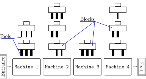
La constitution de lignes de transfert permet de réaliser plusieurs tâches en même temps par la même tête d’usinage. Chaque poste (machine) contient une ou plusieurs têtes d’usinage (blocs), les têtes de chaque poste sont activées de manière séquentielle, les stations comme précédemment sont synchronisées par un convoyeur unique commun. Ainsi, le problème de l’équilibrage de la ligne de transfert consiste en l’attribution de tâches de production à des têtes d’usinage et à la distribution de têtes aux machines répondant à toutes les contraintes. Le critère d’optimisation est la robustesse mesurée par le rayon de stabilité. Seules les métriques ℓ1 et ℓ∞ sont prises en compte pour son calcul.
Nous formalisons le calcul de ces métriques par l’intermédiaire d’une série de lemmes et de théorèmes. Ensuite, deux nouveaux modèles mathématiques sont présentés. Leur complexité nécessite quelques améliorations pour une exécution efficace. Sur la base de pratiques bien connues concernant les problèmes d’équilibrage de ligne, nous introduisons des intervalles d’affectation des tâches sur des lignes de transfert. Cet intervalle affiche les index des blocs pouvant exécuter la tâche considérée. Cinq règles sont élaborées pour calculer ces intervalles pour deux métriques différentes et sont appliquées dans une approche appelée Reduction.
Une méthode heuristique pour les lignes de transfert est élaborée. Outre l’idée, qui s’apparente aux méthodes classiques de lignes d’assemblage, nous devons prendre en compte la construction de blocs. Pour éviter l’attribution répétitive de tâches, qua-tre procédures avec différentes restrictions sont construites. Ensemble, elles composent un algorithme heuristique à démarrages multiples qui, à chaque itération, recherche un équilibrage linéaire avec un rayon de stabilité supérieur à la plus grande valeur connue. Tous les développements présentés constituent l’approche globale de pré-traitement, qui génère non seulement une solution initiale et une borne inférieure, mais crée également deux familles d’inégalités pour enrichir les formulations PLNE.
Tous les modèles et algorithmes de pré-traitement sont programmés avec C++ et résolus par le solveur commercial Gurobi. Les données d’instance ont été importées de la bibliothèque d’exemples générés aléatoirement pour les lignes de transfert. Les résul-tats prouvent l’hypothèse centrale selon laquelle la densité du graphe de précédence a un impact significatif sur la résolution du problème. En général, la méthode présentée montre une capacité à résoudre des instances dont la taille est équivalente aux résultats précédemment rapportés dans la littérature relative aux lignes de transfert.
Approches de solutions hybrides pour le problème d’équilibrage de
ligne de transfert
Cette approche consiste en une application combinée d’un solveur PLNE commer-cial et d’algorithmes de génération de coupes basés sur l’optimalité. Nous utilisons des techniques de callback qui permettent de gérer et de guider le processus d’optimisation. Deux solveurs commerciaux sont considérés afin de trouver celui qui conduit à la résolu-tion la plus efficace. Plusieurs types de callbacks sont étudiés. Nous avons choisi deux approches possibles pour la génération de coupes avec les callbacks. Ils reposent sur la technologie dite des lazy constraints et le MIP restart, respectivement. L’approche par les lazy constraints fonctionne avec un ensemble de coupes qui est introduit progressivement dans le modèle à résoudre. Dans ce cas, les callbacks n’interrompent pas la résolution, et le solveur reprend son travail après l’insertion des coupes basées sur l’optimalité. Les métriques ℓ1 et ℓ∞ ont nécessité des implémentations distinctes en raison d’une
interpré-tation différente du rayon de stabilité. Comme pour la méthode de prétraitement globale, nous utilisons la méthode Reduction pour déterminer les intervalles d’affectation et les blocs inutilisés sur les machines.
La solution hybride est programmée en C++ et résolue par le solveur commercial GUurobi pour les tests finaux. Des expériences ont été menées sur un nombre plus réduit d’instances qu’au chapitre 3. L’approche MIP restart a montré son avantage par rapport aux lazy constraints et aux opportunités de recherche et développement futurs.
Perspectives
Tous les résultats obtenus révèlent de nombreuses perspectives pour les recherches futures sur l’optimisation robuste des chaînes de production.
• Tout d’abord, nous avons plusieurs options pour améliorer les modèles PLNE en utilisant des techniques avancées de solveurs commerciaux. Mais même dans ce cas, il existe un risque de se heurter à des limites strictes qui ne permettront pas de trouver une solution optimale pour des instances de grande taille. L’une des clés de la résolution de ce problème réside dans le développement de méta-heuristiques telles que : les calculs évolutifs, les algorithmes génétiques et l’optimisation d’essaims de particules.
• D’un autre côté, nous pouvons développer des méthodes exactes efficaces pour trou-ver une solution optimale au problème. La littérature comprend de nombreux
exem-ples d’algorithmes de branch-and-price et de branch-and-bound pour les problèmes d’équilibrage de ligne.
• Une estimation de bornes superieures pour le problème d’équilibrage de ligne de transfert pourrait être divisée en deux étapes : la détermination des blocs et leur affectation aux machines. Cela rend impossible l’application de certaines formules classiques au calcul puisque la première étape consiste en général en un problème N P-difficile.
• Notre technique de pré-traitement du problème d’équilibrage de la ligne de trans-fert fait particulièrement référence à la méthode bien connue appelée kernelisation. Il s’agit de pré-traitements au cours desquels les entrées de l’algorithme sont rem-placées par des entrées plus petite (noyau). La simplification de la saisie aide les décideurs, car ceux-ci ne disposent pas toujours d’informations exhaustives au stade de la conception. Ainsi, les développements futurs dans ce domaine ont une signifi-cation pratique indéniable.
• Un certain nombre de méthodes de recherche opérationnelle ont fait leur preuves dans la programmation par contraintes. Cette évolution est tout à fait naturelle, car leurs objetcifs ont souvent les mêmes. D’autres schémas d’hybridation décom-posent le problème afin que CP et OR puissent attaquer les parties du problème auxquelles ils conviennent le mieux. Cette combinaison peut apporter des avantages informatiques substantiels.
• Nous avons pris en compte deux mesures (ℓ1 et ℓ∞) pour calculer le rayon de stabilité
dans le problème d’équilibrage de la ligne de transfert et une autre (résilience rela-tive) dans le problème d’équilibrage de la ligne d’assemblage simple. Cependant, sa définition classique est basée sur le concept de norme, qui a diverses expressions en science. Par exemple, il existe de nombreuses manières de mesurer la différence entre deux séquences (voir les distances de Levenshtein, Hamming, Lee et Jaro–Winkler). Elles ouvrent des possibilités d’estimation de la stabilité des systèmes de fabrication reconfigurables (y compris les chaînes de production), dont la popularité ne cesse de croître ces dernières années.
Dans cette thèse, nous traitons le problème de la conception de lignes de production en présence de temps de traitement sujets à des incertitudes. Cependant, le problème de la prise en compte de l’incertitude des données au stade de la conception ne se limite pas à la prise en compte des variations de ces données numériques. Ainsi, des modifications possibles peuvent également se produire au niveau de diverses contraintes, telles que les contraintes de précédence. Jusqu’à présent, cet aspect n’est pas encore bien été traité dans la littérature. Ceci est une piste de nos recherches futures dans ce domaine.
Contents
Résumé de la thèse
List of Figures xv
List of Tables xvii
Introduction
Chapter 1 Line Balancing under Uncertainty
1.1 Production lines . . . 5
1.1.1 Basic terms of production lines . . . 6
1.1.2 Types of production lines . . . 7
1.1.3 Line balancing . . . 10
1.2 Modelling of uncertainty . . . 14
1.2.2 Fuzzy approaches . . . 19
1.2.3 Robust approaches . . . 21
1.3 Stability radius maximisation . . . 25
1.4 Conclusion . . . 27
Chapter 2 Robust Balancing of Simple Assembly Lines 2.1 Constitution of an assembly line in introduced notations . . . 30
2.2 MILP formulations . . . 33
2.2.1 MILP formulation for ℓ1-metric . . . 35
2.2.2 MILP formulation for ℓ∞-metric . . . 35
2.2.3 MILP formulation for ℓrr-metric . . . 36
2.3 Enhancements . . . 37
2.4 Polynomial time solvable case . . . 37
2.5 Computational results . . . 38
2.6 Conclusion and perspectives . . . 42
Chapter 3 Robust Balancing of Transfer Lines 3.1 Constitution of a transfer line . . . 44
3.2 Stability radius . . . 45
3.2.1 Save time . . . 48
3.2.2 Calculation of stability radius for ℓ1-metric . . . 49
3.2.3 Calculation of stability radius for ℓ∞-metric . . . 50
3.3 MILP formulations . . . 53
3.3.1 Complexity . . . 53
3.3.2 MILP formulation for P1 . . . 53
3.3.3 MILP formulation for P∞ . . . 55
3.4 Pre-processing . . . 57
3.4.1 Assignment intervals and empty blocks . . . 57
3.4.2 Heuristics . . . 62
3.4.3 Global pre-processing approach . . . 64
3.5 Computational results . . . 66
3.6 Conclusion . . . 70
Chapter 4 Hybrid solution approaches for TLBP 4.1 User callbacks in modern solvers . . . 74
4.1.1 IBM CPLEX 12.7 . . . 75
4.1.2 GUROBI 7.51 . . . 75
4.2 Cuts generation with callbacks . . . 76
4.2.1 Lazy constraints . . . 76 4.2.2 MIP restart . . . 78 4.3 Computational results . . . 80 4.4 Conclusion . . . 83 General Conclusion Bibliography Appendixes 97
Appendix A Simple assembly lines. Detailed computational results 97 Appendix B Simple assembly lines. Detailed instances 109 Appendix C Transfer lines. Detailed computational results 115 Appendix D Hybrid approach with callbacks. Application for TLBP 147
List of Figures
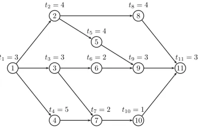
1.1 Precedence graph . . . 7
1.2 Scheme of a paced production line . . . 8
1.3 Scheme of an unpaced production line . . . 8
1.4 Line balance . . . 11
1.5 Line balance with certain and uncertain tasks . . . 13
1.6 Deviated line balance . . . 13
1.7 A membership function for a fuzzy set . . . 20
1.8 Robust line balance . . . 26
2.1 Precedence constraints of the instance JACKSON . . . 40
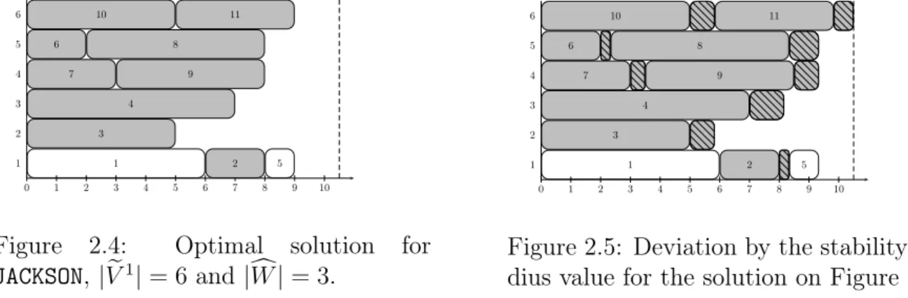
2.2 Optimal solution for JACKSON, |]V1| = 6 and |[W | = 0. . . 40
2.3 Deviation by the stability radius value for the solution on Figure 2.2 . . . . 40
2.5 Deviation by the stability radius value for the solution on Figure 2.4 . . . . 40
3.1 Scheme of a transfer line with four machines . . . 45
3.2 Example of assignment . . . 47
3.3 Stability radius for ℓ1-metric . . . 47
3.4 Stability radius for ℓ∞-metric . . . 48
3.5 Block with uncertain tasks having zero save time . . . 48
3.6 Block with uncertain tasks having non-zero save time . . . 48
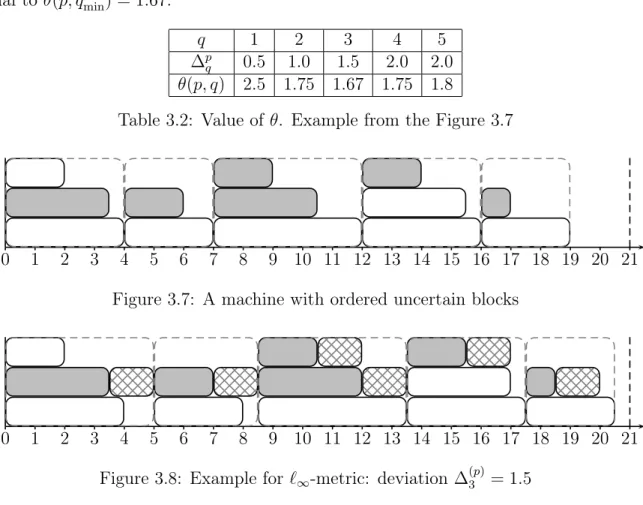
3.7 A machine with ordered uncertain blocks . . . 52
3.8 Example for ℓ∞-metric: deviation ∆(p)3 = 1.5 . . . 52
List of Tables
2.1 Solving Prr with GUROBI for | eV1| = ⌈n4⌉ and |cW | = 0 . . . 39
2.2 Comparison of results for JACKSON . . . 41
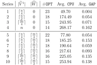
2.3 Summary results for all series . . . 42
3.1 Basic notations for TLBP . . . 46
3.2 Value of θ. Example from the Figure 3.7 . . . 52
3.3 Intervals Qj for Example 2 . . . 61
3.4 Intervals Qj for Example 2 with dynamic improvements . . . 62
3.5 Main characteristics of Series S1, S2 and S3 . . . 66
3.6 Computational results for basic models with rmax= 2 . . . 67
3.7 Computational results for basic models with rmax= 3 . . . 67
3.8 Results with the heuristics and the cuts with rmax= 2. . . 68
3.10 Results with the heuristics and the cuts with rmax = 3. . . 70
4.1 Example of detailed results for the hybrid approach . . . 81 4.2 Improvements of Lazy constraints over MIP restart in terms of gap and CPU time 82 4.3 Average results in ℓ1 metric . . . 83
4.4 Average results in ℓ∞ metric . . . 84
A.1 Results for | eV1| = ⌈n
4⌉ and |cW | = 0 . . . 98
A.2 Results for | eV1| = ⌈n
2⌉ and |cW | = 0 . . . 99
A.3 Results for | eV1| = ⌈3n
4 ⌉ and |cW | = 0 . . . 100
A.4 Results for | eV1| = n and |cW | = 0 . . . 101
A.5 Results for | eV1| = ⌈n
4⌉ and |cW | = ⌈ m
4⌉ . . . 102
A.6 Results for | eV1| = ⌈n
4⌉ and |cW | = ⌈ m
2⌉ . . . 103
A.7 Results for | eV1| = ⌈n
2⌉ and |cW | = ⌈ m
4⌉ . . . 104
A.8 Results for | eV1| = ⌈n
2⌉ and |cW | = ⌈ m
2⌉ . . . 105
A.9 Results for | eV1| = ⌈3n
4 ⌉ and |cW | = ⌈ m
4⌉ . . . 106
A.10 Results for | eV1| = ⌈3n
4 ⌉ and |cW | = ⌈ m
2⌉ . . . 107
C.2 Series 2. 2 tasks per block . . . 121 C.3 Series 3. 2 tasks per block . . . 126 C.4 Series 1. 3 tasks per block . . . 131 C.5 Series 2. 3 tasks per block . . . 136 C.6 Series 3. 3 tasks per block . . . 141 D.1 Callbacks. Restart. 2 tasks per block . . . 148 D.2 Callbacks. Lazy. 2 tasks per block . . . 151 D.3 Callbacks. Restart. 3 tasks per block . . . 154
Introduction
In the contemporary industry, manufacturing systems play a crucial role. The world’s population is increasing, creating a growing demand for products and services. To meet this demand and take the challenge of competition, each company must carefully design its manufacturing system that will be both effective for the quality of manufactured products and the capital expended. One of the most common manufacturing systems in the industry is the production line, it consists of stations aligned sequentially. Decisions related to the design of the production lines are of great importance because the cost of setting up a production line is in the millions of euros.
The design of production systems includes several steps. We are particularly in-terested in the stage of balancing the production line. For a given set of workstations, this step follows the analysis of the products to be manufactured and the planning of the manufacturing process which determine the information about the work processing in the designed system, i.e., a set of indivisible tasks related by some constraints. These constraints come from technological, economical and environmental considerations or er-gonomic factors for the workforce. Line balancing consists of choosing the resources of and assign them to the workstations, so that all constraints are satisfied and predefined objectives are met. Traditionally, these objectives can be, for example, to minimise the total cost or to maximise the productivity of the line. Problems occurring at the config-uration stage manufacturing lines are combinatorial in nature. The designer of the line is looking for the optimal solution(s) among other feasible solutions. It is a difficult task as the number of feasible solutions is huge, so the choice of an appropriate method to tackle this problem is decisive. The selected method is expected to return high-quality solutions at a reasonably low computational cost. Moreover, some uncertainties, which may compromise the feasibility of a solution, must be taken into account in order to avoid this pitfall.
In this thesis, we consider the production line balancing problem under uncertainty. It consists of assigning of production tasks to the fixed number of stations, such that the line is going to work with a given production rate determined by cycle time. The cycle time shows how fast the line produces a new piece of product. All tasks are supported by an estimated processing time and a set of constraints determining their order on the line. We assume that task processing times can deviate in the future according to product characteristic changes, employee fatigue and experience or something else. These events
may compromise solution feasibility, or deteriorate performance, so the stability of the line balance is the problem objective. Our goals are to develop an effective method for maximising the line ability to maintain feasibility despite task time deviation, and to show its application for simple assembly and transfer lines. The proposed method consists in studying a new alternative approach, introduced in recently appeared works on robust optimisation, that is more appropriate for handling uncertainty in the field of production systems than those used up to now. This leads us to investigate new industrial optimisation problems representing an essential object of study from both practical and algorithmic points of view. In what follows, we present the structure of the thesis, which is made of four chapters.
Chapter 1 presents the study of existing production lines, their parameters and at-tributes. We show which types of production lines exist and why it is important to know how to balance them. Three common objective functions minimising the number of sta-tions, cycle time and line efficiency are highlighted. Events modifying processing times of tasks are considered. Their impact on a line balance and its productivity is pictured in series of examples. Possible task time deviations have to be taken into account at the design stage in order to keep the line working after installation. We consider uncertainties that can be faced during the line balancing process. In the second part of the chapter, we analyse existing approaches to model data uncertainty in combinatorial optimisation problems. We identify the robust one that best fit the context of the design of production lines. It is based on the stability radius, which shows the maximal value of processing time deviations that do not violate solution feasibility or optimality. In the end, we introduce a new robust formulation for the production line balancing problem.
Chapter 2 is related to Simple Assembly Lines, which consist of stations synchro-nised by a common conveyor. Robust versions of the simple assembly line balancing problem consider that the number of stations and the cycle time are fixed parameters. The problem is to allocate assembly tasks to stations satisfying all manufacturing con-straints and maximising the robustness measured by the stability radius. We analyse two classic metrics for its calculation and introduce a new one representing the case of the proportional robustness. Respective theorems and formulas are established. Based on them, we propose combined mixed-integer linear programming models, which are aimed to help decision-makers easily switch from one model to another according to the partic-ular situation and available knowledge. Several enhancements are following the studied models. Among them, a greedy heuristic method, some combinatorial upper bounds, and a cut generation method. Computational results and conclusion are finishing the chapter. In Chapter 3 we adapt our method for the generalised case of assembly lines, referred to in the literature as Transfer Lines where several tasks can be performed simultaneously by a single machining head. Each station (machine) contains one or more machining heads (blocks), the heads of each station are activated sequentially, the stations as before are synchronised by a common conveyor. This major difference from simple assembly lines determines new properties that makes mathematical models more complex. The transfer line balancing problem consists in assignment of production tasks to machining heads and
distribution of heads to machines satisfying all given constraints and maximising the value of the stability radius. We discover new formulas for measurement of line robustness in Manhattan and Chebyshev metrics and prove them within a series of lemmas and theo-rems. Two Mixed Integer Linear Programming (MILP) models are developed according to all problem properties. To handle their complexity, we proposed some enhancements based on well-known practices for line balancing problems. First of all, we introduce assignment intervals of tasks and introduce five rules to calculate them under both the considered metrics. Together with a reworked heuristic algorithm they compose a global pre-processing approach which not only generates an initial solution and a lower bound, but also creates two groups of constraints for MILP formulations. The chapter is ending by computational experiments.
Chapter 4 presents a new hybrid approach for transfer line balancing problem. It is aiming to reduce the search space during the optimisation process by generation of opti-mality based cuts. We study advanced technologies of commercial solvers called callbacks. Solvers IBM CPLEX and Gurobi are considered for a better understanding of possible options and approaches. Two implementations (MIP restart and lazy constraints) are analysed and explained in details. Within both of them, we explain applications for de-veloped models. Computational results compare implementations with each other and with enhanced MILP models.
Chapter 1
Line Balancing under Uncertainty
Contents
1.1 Production lines . . . 5 1.1.1 Basic terms of production lines . . . 6 1.1.2 Types of production lines . . . 7 1.1.3 Line balancing . . . 10 1.2 Modelling of uncertainty . . . 14 1.2.1 Stochastic approaches . . . 14 1.2.2 Fuzzy approaches . . . 19 1.2.3 Robust approaches . . . 21 1.3 Stability radius maximisation . . . 25 1.4 Conclusion . . . 27
1.1
Production lines
Production lines are present in different industrial environments and are widely used to manufacture a large variety of products. Primarily, they are used to produce consumer goods such as cars, engines, domestic appliances, television sets, computers, smart-phones, and other electrical devices. Since the production constraints can vary a lot according to the products, the corresponding production systems can present major differences. Consequently, the literature includes a wide range of balancing problems. In this section, we examine characteristics that determine various types of production lines.
1.1.1
Basic terms of production lines
A task is a simple portion of the total work content in a production line. The time required to perform a task is called processing time (of a task). We assume that tasks are indivisible, i.e., they cannot be split into smaller work elements without creating unnecessary additional work.
A station (or workstation) is a segment of the production line where a certain amount of tasks is executed. It is characterised by its dimension, the machinery, and equipment as well as the kind of assigned work. There are two types of stations: manual and automated. The manual station or workplace has to be occupied by a human operator, who performs work using either a simple tool or semi-automated machines which have to be controlled by an operator. Automated stations or machines can work by themselves. We do not consider independently a group of collaborative stations, which are hybrids with human and machine (robot) working together. Their applications in manufacturing are usually presented by co-existence or sequential collaboration. In both, human and robot do not work on a production part at the same time. Thus, mathematical representation may interpret a collaborative station as two independent: one manual and one automated. The set of tasks assigned to a station is referred to as station load, the time necessary to perform the work as load time (of a station).
The material handling system is the mechanical equipment used for the move-ment, storage, control and protection of workpieces or production parts throughout the process of manufacturing. A conveyor belt is a common choice for production lines.
The cycle time represents the duration that separates the release of two products in a permanent regime. On a paced production line this duration is equivalent to (or at least not smaller than) the load time of the most charged station. On an unpaced one, this value has no direct references to stations and their load times. See the differences between paced and unpaced lines below in this chapter. The production rate is the division of a one-time unit by the cycle time. The distance between the cycle time and the load time is called idle time (of a station).
Precedence Constraints show some technological restrictions between tasks. They are usually represented by an acyclic oriented graph, where each node models a task. A given precedence graph may have several source and final nodes if there is no special type asked by an industrial environment. The interpretation of arcs depends on particular cases, but, in general, an arc (i, j) indicates that the task j must not be completed before the task i can start, and cannot be assigned to an earlier station than i. An example of a precedence graph appears in Figure 1.1. Here the task 4 cannot be performed earlier than any of its predecessors 1, 2 or 3; as well as later than any of its successors 6, 7 or 8. Similarly, there is no connection with task 5; thus, the order of their appearance on the line is free.
1.1. Production lines 1 3 2 4 5 6 7 8
Figure 1.1: Precedence graph
1.1.2
Types of production lines
Number of products
The first characteristic is the number of different products released by the same production line. The literature distinguishes the following line types.
Single-model lines: A single product type is manufactured at the line in large quantities. A set of production tasks is known. All stations repeatedly have to perform the same subset of tasks on identical workpieces.
Mixed-model lines: several models of a basic product are manufactured on the same line (but not at the same time). The models differ from the primary one only concerning some attributes and optional features. The production processes are quite similar in this case and, consequently, the same set of basic operations is necessary to produce any of the models. The presence or absence as well as processing time of a task depends on an optional part being installed or not and on its parameters. Minor setup activities are applying to switch from one model to another.
Multi-model lines: several products are manufactured on the same line in separate batches. Significant differences in production processes require major setup activities (or rearrangements) of the line equipment when products are changing. Besides processing time variations, setup times are taking into account.
Product Flow Manner
A production line consists of stations and a material handling system, which connects stations and moves production parts from one station to the next one. It also determines how elements flow through the line.
Paced lines: material handling systems as conveyor belts flexibly connect the sta-tions. Production parts are steadily moved between stations by the conveyor belt at constant speed immediately after being processed. Each station has the same amount of available working time (the cycle time) to perform the assigned tasks on all incoming
workpieces. Figure 1.2 illustrates a paced production line with four stations. Station 1 Station 2 Station 3 Station 4
Production parts E nt ra nc e E xit
Figure 1.2: Scheme of a paced production line
Unpaced lines: the stations are separated by buffer stocks which hold production parts when previous items still occupy the following stations. Usually, buffers have limited capacities. Because of this, a station may be blocked when the following buffer is full. Conversely, a station is starving when the preceding buffer is empty after terminating its assigned tasks. Thus, buffer sizes directly impact the production rate of the line. An illustration of an unpaced line is presented in Figure 1.3. There are three stations with two buffers in between. Station 1 could be blocked since the following buffer is full, while station 3 is going to be idle if station 2 did not release its production part in time.
Station 1 Buffer Station 2 Buffer Station 3 Production parts E nt ra nc e E xit
Figure 1.3: Scheme of an unpaced production line Line layout
Basic Straight: this is a traditional layout of production lines. Each workpiece visits a series of stations in order of their installation. The tasks on stations are supposed to be executed sequentially one by one.
Straight with multiple stations: the advantages of parallelisation can be used to increase productivity in a single line by installing multiple stations, i.e., the production parts are distributed among several operators or automated tools which perform the same
1.1. Production lines tasks. It helps to reduce the (actual) cycle time of the entire system if some tasks have processing times longer than the desired cycle time. Such tasks should be assigned to parallel stations.
U-shaped: these lines have both the entrance and exit in the same place. They are commonly manual. Workers placed between two legs of the line are allowed to walk from one leg to another. Therefore, they can work on two (or more) workpieces during the same cycle. Stations are closer together such that visibility of the production process, and communications between operators are improved.
Lines with circular transfer: stations are dispatched around a rotating table which is used for loading-unloading and moving the part from a station to another. Concerning the number of turns during which a part stays on the table before being completed, the lines with a single circular transfer can be distinguished. If only one part side is handling at each station and a single turn is sufficient for completing a product, then this configuration is equivalent to a basic straight line. If several sides of the part could be treated simultaneously, then this configuration is equivalent to a line with multiple stations. For the case of multi-turn transfer, the set of tasks assigned to a station must be partitioned into the different cycles corresponding to the number of turns of the table. Asymmetric: they can be used to postpone the differentiation of products to main-tain a typical line configuration for all manufactured products as long as possible. This strategy reduces the risks associated with increasing product variety, but the correspond-ing line balanccorrespond-ing problem must be solved conjointly with a layout optimisation problem in order to determine the final line configuration.
Multiple lines using multiple lines can offer several advantages. Investments can be deferred because additional lines can be installed one by one as they are needed. Production can be adapted more quickly to meet changes in demand. Failure of one line does not necessarily adversely affect the rhythm of other lines, and production costs may be reduced, among other advantages. One drawback is the increased investment cost compared to a single line. The consequences for worker productivity can be diverse: a longer line cycle time in the case of multiple lines enriches the work and improves motivation. However, this may limit the learning effect, since the variation of operations performed by a worker increases. Therefore, the choice between a single line with short cycle time and many lines with longer cycle times is not straightforward and should be considered as a part of an integrated decision-making process.
Industrial environment
Assembly: a final product is assembled from different components. These lines have many different applications from manual with worker assignment to fully automated.
Disassembly: the objective is to separate end-of-life (EOL) products subassemblies and components for recycling, remanufacturing and reuse. Such lines are used to carry out disassembly operations with higher productivity rate. The structure and quality of EOL products are strongly uncertain and even the number of components in such products can not be predicted. Moreover, the precedence graph cannot be obtained by reversing a relevant one for the assembly line. That makes disassembly process more complex than assembly. Due to technical or economic restrictions such as irreversible connections of components of a product and low revenue obtained from retrieved parts, disassembly lines are mostly manual today.
Machining: a product is completed by a series of machining operations like drilling, milling, reaming, and other. In general, there may be much fewer precedence relations between such operations than in the case of an assembly or disassembly process. However, there may exist many tolerance constraints that impose assigning operations to the same workstation and incompatibility constraints that forbid the assignment of specific tasks to the same station because of technological incompatibilities. Such lines are usually highly automated.
1.1.3
Line balancing
Line balancing is a stage of the design that consists in finding an assignment of production tasks among stations that satisfies all the constraints of the problem in order to optimise one or several goals.
A Line Balance is a feasible solution to a balancing problem. For the feasibility, a solution has to satisfy several constraints: each task is assigned to exactly one station; precedence constraints are fulfilled; the load time of any station does not exceed the cycle time. A line balance is optimal if, besides the restrictions, it also maximises (minimises) given production goals (objectives).
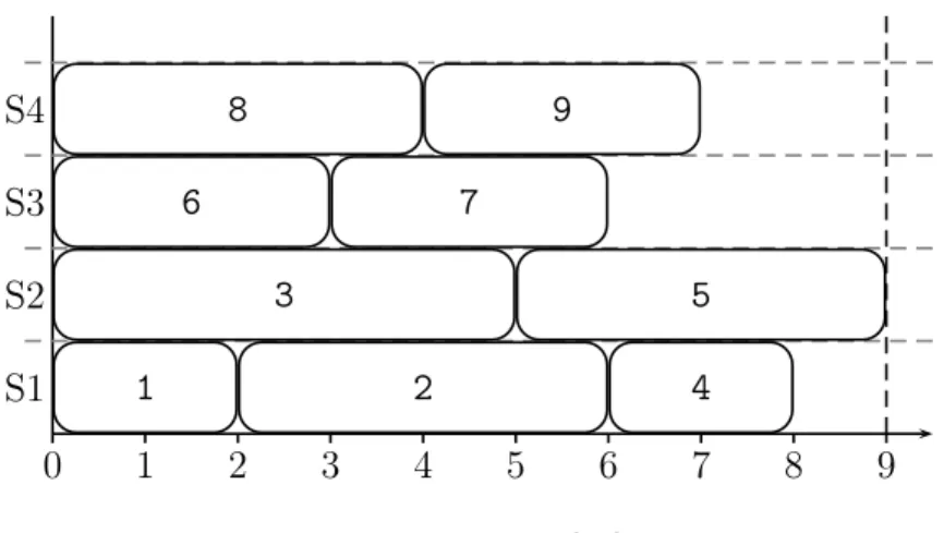
Example 1. A line balance is shown in Figure 1.4 as a Gantt chart, where four stations process nine tasks. One layer includes all tasks assigned to the same station. Processing times are equivalent to lengths of rectangles. The most loaded station determines the cycle time (9, by station S2). The idle times are 1, 0, 3 and 2 for stations S1, S2, S3 and S4 respectively. The balance also presents the order of tasks execution on the stations. Thus, station S1 (or a worker assigned to it) performs the task 1, then task 2, and task 4 in the end. At time 9, a conveyor belt moves a production part to station S2. Station S2 starts the task 3, and then task 5, and so on until the end of the production line.
1.1. Production lines 0 1 2 3 4 5 6 7 8 9 S1 S2 S3 S4 1 2 4 3 5 6 7 8 9
Figure 1.4: Line balance
capital investments. Therefore, it is vital for a designed system to be as efficient as possible. A new line balanced before launching has to be re-designed later according to a periodically (planned) or single changes in the production process. The objectives have to be carefully chosen, according to the goals of the company to minimise the long-term effect of balancing (re-balancing) decisions. Traditionally, there are three types of line balancing problems:
• type-1: minimise the number of stations for a given cycle time; • type-2: minimise the cycle time for a given number of stations;
• type-E: minimise the line efficiency represented by the non-linear function – the product of the number of stations and the cycle time, while they are given by lower and upper bounds.
Now, when we have an understanding about line balance and production goals, let introduce some helpful notations:
• V = {1, 2, . . . , n} is a set of production tasks to be assigned; • tj is a nominal processing time of the task j, j ∈ V ;
• m is a number (maximal) of available stations; • T is a cycle time;
• G = (V, A) is a precedence graph, where A is a set of arcs (i, j), such that i, j ∈ V . Then, deterministic models can be introduced with following constraints:
m
X
k=1
m X k=1 kxi,k ≤ m X k=1 kxj,k, ∀(i, j) ∈ A, (1.2) X j∈V tjxj,k ≤ T yk, ∀k = 1, 2, . . . , m, (1.3) yk ∈ {0, 1}, ∀k = 1, 2, . . . , m, xj,k ∈ {0, 1}, ∀j ∈ V, ∀k = 1, 2, . . . , m. (1.4)
Restrictions 1.1 assure that any production task assigned exactly to one station. The precedence order is modelled in 1.2. The load time of any station does not exceed the cycle time, as it is shown in 1.3. Two last groups represent constraints on variables:
• xj,k is a decision variable, that equals to 1 if and only if the task j is assigned to the
station k;
• yk states if the station k is presented on the line.
Objective goals mentioned above can be written in mathematical form as: • type-1: minimise m P k=1 yk; • type-2: minimise T ; • type-E: minimise T · m P k=1 yk.
Regardless of the type of production line and objectives, new challenging conditions or changes may arise during the manufacturing process. Their prediction or, at least, anticipation is a substantial part of the line balancing stage. The changes that affect sta-tions availability and task processing time posses the major challenges. Indeed, a human operator cannot work with constant speed due to several reasons, such that: personal experience, proficiency, education, fatigue, health conditions, partial dissatisfaction with something, thrill before the holidays, or something else. Even tasks executed by a ma-chine may not have a stable processing time because of overheating, material or product specification changes, malfunctioning, the input lag of software. All of these events may inflict costly damage and should be prevented within the line balancing. For this purpose, we assume that all tasks are belonging to one of two subsets: certain and uncertain. Cer-tain ones have a fixed processing time that is not affected by any event. On the contrary, uncertain tasks are vulnerable, and their processing time is changing with an occasion on the line.
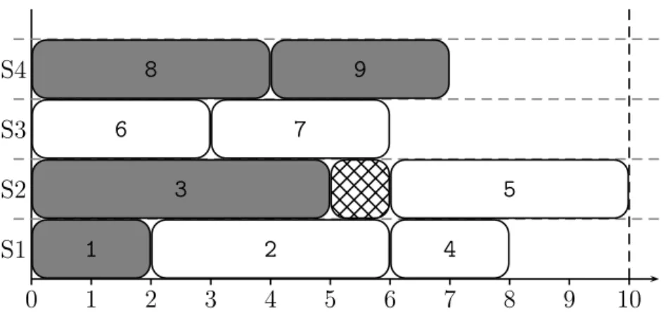
1.1. Production lines Example 2. Consider the line balance from Figure 1.4. Assuming that tasks 1, 3, 8 and 9 are uncertain, they are coloured in grey, as shown in Figure 1.5. In paced mode the line produces a new piece of product every 9 units of time. If a unit of time equals to one second, then the production rate is 400 pieces per hour. Now, imagine that because of a worker replacement or mistaken estimation the processing time of the task 3 is increasing from 5 to 6 units of time. Figure 1.6 shows the deviated line balance. The new cycle time is 10, which is equivalent to the production rate of only 360 pieces per hour, which amounts to a significant throughput loss. Moreover, if the line is automatic and the cycle time is strongly fixed, then such deviation will cause the line interruption. Thus, anticipation of task time uncertainties should be taken into account at the design stage.
0 1 2 3 4 5 6 7 8 9 S1 S2 S3 S4 1 2 4 3 5 6 7 8 9
Figure 1.5: Line balance with certain and uncertain tasks
0 1 2 3 4 5 6 7 8 9 10 S1 S2 S3 S4 1 2 4 3 5 6 7 8 9
1.2
Modelling of uncertainty
In this section, we discuss some approaches which are used to handle task time uncertainties in line balancing problems. Detailed general observations on a line balancing are given by Scholl and Becker [63], Boysen et al. [10], Battaïa et al. [4]. Earlier comprehensive surveys about line balancing under task time uncertainty was published by Bentaha et al. in [9] and [8]. The literature usually considers three major approaches: stochastic, fuzzy and robust methods.
1.2.1
Stochastic approaches
Stochastic approaches are the most popular ones and consist of a representation of task times as independent random variables with known characteristics, usually symmetric distribution.
Chance-constrained programming
This approach presents the processing time of tasks as normally distributed indepen-dent random variables tj ∼ N (µj, σj2), j ∈ V . The mean µj and variance σj2 are known
for all tasks. Let us introduce Y = P
j∈V
tj, i.e., a normally distributed random variable
Y ∼ N (P
j∈V
µj, P j∈V
σ2
j). This variable can be easily converted into a standard distribution
using the transformation Z =
Y−P j∈V µj r P j∈V σ2 j
. A designed line balance should respect the cycle time with a given probability α. In practice and literature, this value usually is greater than 0.9. Thus, P(Y ≤ T ) ≥ α, and using mentioned transformation we get the next formula: P Z ≤ T − P j∈V µj r P j∈V σ2 j ≥ α (1.5) P(Z ≤ zα) = α, zα is (100α)-percentile of the standard normal distribution. Expression
(1.5) holds if and only if
zα ≤ T − P j∈V µj r P j∈V σ2 j (1.6) or X j∈V µj+ zα sX j∈V σ2 j ≤ T. (1.7)
1.2. Modelling of uncertainty Let xj,k be a binary variable that is set to one if and only if the task j is allocated to
the station k. Then inequality (1.7) can be written as follows: X j∈V µjxj,k+ zα sX j∈V σ2 jxj,k ≤ T. (1.8)
This expression represents the cycle time constraint that should be satisfied during the design in any type of line balancing problem.
It is evident that a mathematical model with the constraint (1.8) is non-linear which may prevent to successfully solve large problem instances. Thus chance-constrained pro-gramming requires an additional linear transformation for real-life problem instances. Non-linear part can be eliminated by a squaring procedure by introducing new binary variables and constraints.
The reason why the developed chance-constraint model is not linear is the term r P
j∈V
σ2
jxj,k with task variable. For that reason by eliminating the square-root, linearising
will be possible. So, by squaring both side of the inequality (1.6), including variables from (1.8), the next inequality has been obtained.
(zα)2 ≤ (T − P j∈V µjxj,k)2 r P j∈V σ2 jxj,k !2 (1.9)
While the non-linear situation caused by the term r P
j∈V
σ2
jxj,k has been eliminated
by inequality (1.9), a new non-linear term has appeared with term (T − P
j∈V
µjxj,k)2. The
open form of this term is given by (T −X j∈V µjxj,k)2 = T2− 2T X j∈V µjxj,k+ µ2 1x21,k+ µ1x1,kµ2x2,k+ · · · + µ1x1,kµnxn,k µ1x1,kµ2x2,k + µ22x22,k+ · · · + µ2x2,kµnxn,k · · · µ1x1,kµnxn,k+ µ2x2,kµnxn,k+ · · · + µ2nx2n,k (1.10) Since the variable xj,k is 0 − 1 integer, x2j,k is equal to xj,k. The term (µixi,kµjxj,k) is
the non-linear part of the equation (1.10). Thus, a current transformation technique in the literature has been used to make this part linear
After the variable transformation given in (1.11), the variable uijk is linked to xik
and xjk by the following inequalities:
xi,k + xj,k − ui,j,k ≤ 1, (1.12)
xi,k + xj,k − 2ui,j,k ≥ 0. (1.13)
Another situation to be considered on inequality (1.9) is that the inequality is valid in two different cases. These can be expressed by the inequality below.
|zα| ≤ T − P j∈V µj r P j∈V σ2 j (1.14) Assuming that zα is larger than 0.9 implies that zα is positive, and so the right-hand
side of the inequality (1.14) must be positive, too. For that reason, we have to introduce an additional constraints which is the same as the cycle time constraint at the basic deterministic model (compare to 1.3):
T −X
j∈V
µjxj,k ≥ 0. (1.15)
Then, the inequality (1.8) is replaced by the constraint (1.15), the equality (1.11) together with (1.12–1.13) and:
T2 − 2TX j∈V µjxj,k+ n X j=1 µ2jxj,k + 2 n−1 X i=1 n−1 X j=i+1 µiµjui,j,k− zα2 n X j=1 σj2xj,k ≥ 0. (1.16)
This stochastic approach is well-developed and applied almost for all existing types of production lines: straight ([13], [22], [62], [64]), U-shaped ([1], [2], [6], [29], [55]), two-sided ([14], [53], [54]).
Simulation of problem characteristics and re-balancing
The second category involves the work performed to examine the problem charac-teristics via simulation and to compare the deterministic and stochastic versions of the problem. In these procedures, an initial balance is given, and the objective is to rearrange the tasks to fulfil a substitution with a new item due to customers’ unique requirements. It can be observed that the definition of the category is deeply related to a particular case well known in the literature as a re-balancing problem.
Rearrangements may require the modifications of the whole initial parameters, as well as the modification of a subset only. Because of this, the main difficulty in practical cases is
1.2. Modelling of uncertainty the precise estimation of costs related to all possible tasks movements, a weighted multiple objective function involving both completion and tasks movement associated costs is not introduced. Preferably, two separate objective functions, concerning expected completion costs (EC) and the degree of similarity between initial and new tasks assignments (shortly, mean similarity factor or MSF), are separately introduced. EC is calculated in a similar way as the objective function for type-E balancing problem:
EC = mT +X
j∈V
pjIj, (1.17)
where as before m is the number of machines, and T is the cycle time of a new balance, pj is the probability of not completing task j in the assigned station, Ij is the total
incompletion cost of task j. It includes the value of the task itself and those of its followers in the precedence graph, i.e., the task staying earlier in the order is more worthy. In the same manner as in chance-constrained programming, the probability pj is calculated using
the transformation into a standard form:
pj =P(Z ≤ zj) ∀j ∈ V, (1.18) zj ≤ T − P i∈Vjk µj r P i∈Vjk σ2 j ∀j ∈ V, k | j ∈ Vk
where zj represents the station idle time, with respect to task j. Consequently, Vk is a
subset of tasks assigned to station k; Vjk is a subset of Vk (such that j ∈ Vk) including
both the task j and tasks executed before it in the station k. Here, T is exactly the task time which is not always equivalent to the cycle time. As above, the non-linear part can be eliminated by the squaring procedure which consists in introducing new binary variables and constraints.
The second objective function showing the mean similarity factor (MSF), as it follows from the name, is aiming to compare a given initial line balance with a re-designed one. Two special subsets are introduced for this purpose:
TIBj = {i ∈ Vk0 | j ∈ Vk0 and i 6= j} ∀j ∈ V0
TNBj = {i ∈ Vk | j ∈ Vk and i 6= j} ∀j ∈ V
TIBj is the subset of initial tasks, other than j, belonging to the station k in an initial
balance. In a similar manner, TNBj is also the subset of tasks, but for a new balance. As
it was mentioned above, V may differ from V0 because of product changes and another
requirements. The similarity factor (SFj) of the task j is obtained in
SFj =
|TIBj ∩ TNBj|
|TIBj|
. (1.19)
It is the ratio of number of tasks assigned to the same station as task j in the initial and in the new configuration to the number of tasks assigned to the same station in the initial balance.
When the task j is alone in a station in the given configuration, SFj assumes an
indefinite form 0/0. In this case, the SFj value is set to 0 in assignment procedures so as
to make it less likely that this task will be assigned to a station where tasks belonging to other sets are present. Whilst, in the final MSF evaluation step, where the similarity of the line as a whole is computed, SFj is set to 1 in case the task j is alone both in the
initial and in the new balance, and to 0 otherwise.
Notice that SFj takes a value within the range 0 ≤ SFj ≤ 1. SFj takes the value 0
if none of the tasks assigned to the same station as task j in the initial line balance are assigned to the current station. SFj takes the value 1 if all the tasks assigned initially to
the same station as task j are assigned to the current station. SFj takes a value within
the range (0, 1) for any other subset of the tasks. The more numerous is this subset, the higher is SFj.
The mean similarity factor (MSF) between the new re-balanced line and the initial one is finally evaluated as in
MSF = P
j∈V
SFj
|V | . (1.20) In the presence of several new feasible balances, the highest MSF values address the choice of balances with less tasks movements.
Since one of the first appearance in [57], this approach is generally used for assembly line balancing and can be found in [7], [26], [45], [49], [50], [69].
Alternative procedures
In the third category, there are procedures specifically developed for the stochastic problem. They may partially include ideas from either chance-constrained or simulation approach. For example, Saif et al [61] consider a bi-objective model, where the main goal is to minimise the cycle time (as in type-2 problems), and the supporting goal is to maximise the probability of stations to withstand the limit both individually and together. Zhang et al. [74] also present a bi-objective optimisation method aiming to minimise the cycle time as well as the total processing cost. Kao in his works [42] and [43] optimises a type-1 assembly line constructing the preference order for task assignment under stochastic processing times. Carter and Silverman [12] develop a model with off-line repairs for uncompleted tasks partially based on chance-constrained programming. Another approach with off-line completion is proposed in [22] by Erel et al. Minimisation of the smoothness index together with the design cost associated with labor and equipment requirements is given by Cakir et al. in [11] for a line with parallel stations. Chiang et al. [14] model two-sided assembly lines taking into account mated-stations and optimising a weighted sum of the line length and the number of station. Zheng et al. [76] propose a distribution-free models for disassembly line balancing problem, but still dealing with stochastic tasks.
1.2. Modelling of uncertainty Bowl-phenomenon
Besides these three categories, we can find an approach based on the bowl-phenomenon that arises in unpaced systems. This phenomenon consists in the fact that workload should be allocated according to a strictly concave function (stations in the middle are less utilised than those at the start or the end of the line). It helps to find a size of buffers and their locations in an unpaced system that improves a production rate especially when processing times of tasks are not normally distributed or when they are significantly dif-ferent from each other. Among the latest works, we refer to Das et al. [15], Tiacci [67], Urban et al. [69].
1.2.2
Fuzzy approaches
Another type of task times uncertainty is called fuzzy. The term fuzzy is meant to represent variables, expressions and judgements that have no clear (crisp) values or boundaries. In this case, the given information about the processing times is better introduced as a fuzzy set or a fuzzy number. They can appropriately represent imprecise parameters and can be manipulated through different operations defined on them.
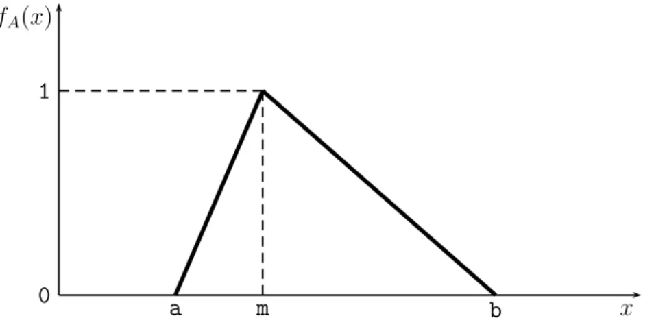
A fuzzy set is defined by a membership function (all the information about a fuzzy set is described by its membership function). The membership function maps elements (crisp inputs) in the universe of discourse (interval that contains all the possible input values) to elements (degrees of membership) within a certain interval, which is usually [0, 1]. Then, the degree of membership specifies the extent to which a given element belongs to a set or is related to a concept. Figure 1.7 shows the membership function of a fuzzy set that represents the concept of “a number close to m”. The crisp input m has a degree of membership in the fuzzy set of one, which means that m is totally related to the concept (it is close to m). Any other number from [a, b] \ {m} has a degree of membership between 0 and 1, which means that a number is partially related to the concept.
The most commonly used range for expressing degree of membership is the unit interval [0, 1]. Thus, for a fuzzy set A, this can be expressed by
fA(x) : X → [0, 1], (1.21)
which means that the membership function fA assigns to each element x of the universal
set X, which is a crisp set, a value within the range [0, 1]. If the value assigned is 0, the element does not belong to the set (it has no membership). If the value assigned is 1, the element belongs completely to the set (it has total membership). Finally, if the value lies within the interval (0, 1), the element has a certain degree of membership (it belongs partially to the fuzzy set). A fuzzy set, then, contains elements that have different degrees
x fA(x)
a m b
1
0
Figure 1.7: A membership function for a fuzzy set
of membership in it. More concrete example, related to Figure 1.7 is written as follows: fA(x) = 0, if x ≤ a, or x ≥ b, λ(x−a) (m−a), if a ≤ x ≤ m, λ(b−x) (b−m), if m ≤ x ≤ b. (1.22) Here, the fuzzy set A is presented by a triplet (a, m, b) of real numbers, such that 0 ≤ a ≤ m ≤ b. The parameter λ shows the maximal possible degree of membership. Sometimes, the inverse of half the length of the segment is used, i.e., λ = 2
(b−a). In this case, the
membership function represents the triangular density of probability.
Initially, necessity of this approach for real production lines was explained by the fact that it is often impractical to use a well-known probability distribution (like Gaussian) to characterise task times. Indeed, for manual production systems where a lot of employees are involved, it is extremely difficult to estimate these densities. Nevertheless, in practice, as a rough estimate, managers are able to provide a usual task time m and 2 values a and b that are, respectively, the lowest and greatest task times. Usually, evaluating a task time using the above three parameters can be enough for most management purposes.
A fuzzy number is a special case of a fuzzy set. Different definitions and properties of fuzzy numbers are encountered in the literature, but they all agree on that a fuzzy number represents the conception of a set of “real numbers close to r”, where r is the number being fuzzified. To classify as a fuzzy number, a fuzzy set A on R must satisfy the following:
• at least one element of the fuzzy set A has full membership; • Aα must be a closed interval for every α ∈ (0, 1], where
1.2. Modelling of uncertainty • The support or scope of A must be bounded.
The concept of α-cut of a fuzzy set is useful for defining the arithmetic operations on fuzzy numbers. As it follows from (1.23), the α-cut is the (crisp) set Aα of elements
x, such that their degree of membership in the set A is at least equal to α (0 ≤ α ≤ 1). To apply this approach, suitable fuzzy arithmetic and an appropriate method ded-icated to comparing these fuzzy sets (numbers) have to be introduced. Because of this, not only the processing times but also another problem data has to be presented by fuzzy sets (the cycle time or number of machines).
In the literature, several fuzzy comparison methods have been proposed such as pseudo-order fuzzy preference model (see Roy and Vincke [59]), fuzzy-weighted average (Vanegas and Labib [70]), signed distance method (Yao and Wu [72]). The last one is the most popular among them, but generally, the fuzzy approach becomes less popular. The following work can be noted: a heuristic method in Hop [40]; a meta-heuristic algorithm for line efficiency maximisation in Zacharia and Nearchou [73]; genetic methods in Tsujimura et al. [68]; binary fuzzy goal programming approach in Kara et al. [44].
During the last four years, the only work that was related to the fuzzy approach is Babazadeh et al. [3]. Authors provide mixed integer linear problem formulations for straight and U-shaped assembly lines and develop a non-dominated sorting genetic algorithm for resolution.
1.2.3
Robust approaches
Evoked in the late 1960s [30], the idea of robustness is attracting increasing interest from both practitioners and theorists in operational research. Originally reflecting a con-cern for flexibility in a context of uncertainty, this concept now seems to fit a much broader spectrum of situations. In the robustness literature, uncertain data is mainly associated with a set, continuous or discrete, of possible values, with no associated probability [46]. In the continuous case, the sets are often intervals, hence the notion of interval approach. In the discrete case, meanwhile, we are talking about the scenario model. Whatever the case, the Cartesian product of these sets defines the possible instances of a problem. After modelling the uncertain data in the form of possible instances, the problem is to find a solution that is “good” for all these instances or robust. We say that a solution is robust if its performance is somehow insensitive to data uncertainty and hazards.
All above-mentioned stochastic techniques require some a priori information to con-struct an appropriate probability distribution and membership function. However, such information is not always available at the design stage due to, for example, originality of the considered line. Since stochastic and fuzzy approaches are hardly applicable, some robust ones have to be used in this case. These approaches assume that only a discrete
set of scenarios or closed intervals of tasks time realisations are available without any distribution on it.
Set of scenarios
Following this definition, a robust solution is then designed to limit or absorb the effects of uncertain data. In practice, it is often considered that the robust solution is the best solution in the worst case. Most of the works on robustness uses the concept of distance between the robust solution calculated a priori and the optimal solution of the instance actually achieved according to a certain criterion (satisfaction of constraints or a particular requirement). In the search for robust solutions, most authors use the criteria of absolute robustness (min-max), maximum regret (min-max regret) or relative regret [60]. For a minimisation problem, if S is the set of possible solutions, I is the set of instances, f(s, I) gives the value of the solution s ∈ S for the instance I ∈ I and f∗ I
the value optimal for instance I ∈ I, then the three criteria are defined as follows: • absolute robustness: min
s∈S maxI∈I f (s, I);
• maximum regret: min
s∈S maxI∈I (f (s, I) − f ∗ I);
• relative regret: min
s∈S maxI∈I
f(s,I)−f∗ I
f∗
I ;
Consider a more precise example for production lines. Let tj,k be the processing
time of the task j on the station k, k ∈ W (W is a set of available stations), and let t be the respective matrix of processing times. It is assumed that t belongs to a set S of scenarios. The set of scenarios S is a finite collection of subsets of interval scenarios: S = S(1)SS(2)S. . .SS(l). Since the set of task processing times is not unique, a question
then appears as to which solution is appropriate. The best solution for one specific set can be the worst for another set. One of the classic approaches to hedge against uncertainty is to construct the best solution for the worst scenario.
The cycle time for this formulation is modelled using the following expression: max t∈S maxk∈W ( X j∈Vk tj,kxj,k ) ≤ T, (1.24) where Vk is a subset of tasks assigned to the station k. This constraint chooses the most
loaded station among all scenarios and checks that its load time does not exceed the cycle time. In case of the type-2 line balancing problem, this approach is exactly representing absolute robustness (or min–max) approach. Its detailed explanation can be found in [21]. Another comprehensive work with new exact and heuristic methods based on the min-max regret approach was given in [56].