HAL Id: hal-02173682
https://hal.inria.fr/hal-02173682
Submitted on 4 Jul 2019
HAL is a multi-disciplinary open access
archive for the deposit and dissemination of
sci-entific research documents, whether they are
pub-lished or not. The documents may come from
teaching and research institutions in France or
L’archive ouverte pluridisciplinaire HAL, est
destinée au dépôt et à la diffusion de documents
scientifiques de niveau recherche, publiés ou non,
émanant des établissements d’enseignement et de
recherche français ou étrangers, des laboratoires
On Chemical Reaction Network Design by a Nested
Evolution Algorithm
Elisabeth Degrand, Mathieu Hemery, François Fages
To cite this version:
Elisabeth Degrand, Mathieu Hemery, François Fages. On Chemical Reaction Network Design by a
Nested Evolution Algorithm. CMSB 2019 - 17th International Conference on Computational Methods
in Systems Biology, Sep 2019, Trieste, Italy. �hal-02173682�
On Chemical Reaction Network Design
by a Nested Evolution Algorithm
Elisabeth Degrand, Mathieu Hemery, and François FagesInria Saclay, Lifeware group, Palaiseau, France
Abstract. One goal of synthetic biology is to implement useful func-tions with biochemical reacfunc-tions, either by reprogramming living cells or programming artificial vesicles. In this perspective, we consider Chemical Reaction Networks (CRN) as a programming language, and investigate the CRN program synthesis problem. Recent work has shown that CRN interpreted by differential equations are Turing-complete and can be seen as analog computers where the molecular concentrations play the role of information carriers. Any real function that is computable by a Turing machine in arbitrary precision can thus be computed by a CRN over a finite set of molecular species. The proof of this result gives a numerical method to generate a finite CRN for implementing a real function pre-sented as the solution of a Polynomial Initial Values Problem (PIVP). In this paper, we study an alternative method based on artificial evolu-tion to build a CRN that approximates a real funcevolu-tion given on finite sets of input values. We present a nested search algorithm that evolves the structure of the CRN and optimizes the kinetic parameters at each generation. We evaluate this algorithm on the Heaviside and Cosine func-tions both as funcfunc-tions of time and funcfunc-tions of input molecular species. We then compare the CRN obtained by artificial evolution both to the CRN generated by the numerical method from a PIVP definition of the function, and to the natural CRN found in the BioModels repository for switches and oscillators.
1
Introduction
One goal of Synthetic Biology is to implement useful functions using biochem-ical reactions, either by reprogramming living cells, or by programming ar-tificial devices. While the former approach is mainstream in synthetic biol-ogy [47,41,19,17,12,1], examples of the later approach are given by the whole field of DNA computing [2,38,11,15,8] or analog computing with enzymatic re-actions [42], possibly encapsulated in artificial vesicles [13].
Chemical Reaction Networks (CRN) are used to describe systems of chemical reactions. In this article, we consider CRN as a programming language [20,46]. We focus on their continuous semantics defined by Ordinary Differential Equa-tions (ODE) on the molecular concentraEqua-tions. We study the CRN program syn-thesis problem, i.e. the problem of designing a CRN for implementing a given function, either a function of time (problem 1) or a function of input molecular species (problem 2):
Problem 1. Given a function f : [0, a] → R, construct a CRN such that one of the species has a concentration A implementing the function f . That is A(t) = f (t), t ∈ [0, a].
Problem 2. Given a function f : [0, a] → R, construct a CRN such that, when initialized for a given input, one of the species converge to the desired result. That is ∀x ∈ [0, a], X(t = 0) = PI(x) ⇒ A(t = 1) = f (x) where X is the vector
of species concentrations and PI a polynomial of degree one.
A recent result proving the Turing completeness of continuous CRN [20], re-stricted to mass action law kinetics and with at most two reactants, has given rise to a numerical method for compiling computable real functions and programs in finite CRN. This approach is implemented in Biocham-41[20] and CRN++2 [46]
with some different design choices. The theoretical result states that one can re-strict to real functions presented as solutions of polynomial differential equations and polynomial initial values as functions of the inputs (PIVP). For a positive PIVP, the transformation can use a CRN inference algorithm from ODEs such as [29] or [21] initially dedicated to importing MatLab models in SBML [25]. For negative variables, the transformation can use the dual-rail encoding of a real variable by the difference between two positive variables for the positive and neg-ative parts respectively [37]. In the generated CRN the molecular concentration play the role of information carriers, similarly to analog computation performed by protein complexes in cells [17,43].
In this article, we study an alternative CRN design method based on artificial evolution, and compare the results to the numerical method. In [15] a complete search method is described for scanning the space of CRN that may implement a given function with a limited number of species and reactions, and then optimiz-ing the kinetic parameters usoptimiz-ing a metropolis like algorithm. This enumerative algorithm is limited to small size CRN with only a handful of species and re-actions. Another method described in [6] consists in sketching a CRN in broad outline and letting an optimization algorithm complete the holes to perform the desired function. This method thus requires prior knowledge on the CRN. In the framework of gene regulatory networks, [33] gives a method to infer network parameters but with also prior knowledge on the structure of the network. In [18] a method to evolve reaction networks is presented using the DNA toolbox and one single genetic algorithm for both structure and parameters.
The method presented here does not require prior knowledge. It is based on artificial evolution with the hope of finding CRN more akin to comparison to natural CRN present in BioModels. The idea is to let an evolutionary algorithm (EA) evolve a population of CRN to approximate a real function given on a finite set of values. These data are either finite traces for approximating a function of time (problem 1), or dose-response diagrams for approximating a function of input (problem 2). The general idea is to let evolve a population of potential CRN while selecting them according to a fitness that is the distance between
1
http://lifeware.inria.fr/biocham4
2
their output and the desired target function. We take here as a distance the L2 norm evaluated in a specified set of points.
Such a CRN design method by artificial evolution can also be seen as a machine learning procedure [45] to learn a CRN from traces either observed in the systems biology perspective, or desired in the synthetic biology perspective. This method may be seen as a learning problem akin to those currently solved with neural networks or linear regression. The input is a set of points (xi, yi)
called data and the goal is to find a function f from a certain class that minimizes the difference between the yi and f (xi). The output of the approximation is the
best function f . However, as the approximation function f is computed through a CRN, we also hope for a network that will gives us some explanatory power in systems biology, as well as some implementability in synthetic biology.
We present a nested evolution algorithm which combines a genetic algorithm for evolving the CRN structures of a population of CRN, with a black-box con-tinuous optimization procedure, namely the covariance matrix adaptation evo-lutionary strategy (CMA-ES) [28], for optimizing the kinetic parameters of the CRN by evolving a population of parameter settings. This nesting of two levels of evolution has been proposed, see for instance [4] for mixed-variable optimization problems in the framework of non-linear optimization problems, refined in [5] to evolve a cell model with structure optimization and parameter optimization. The authors suggest to use a better genetic algorithm for parameter optimiza-tion and to parallelize the genetic algorithms. This is what we show here with the choice of CMA-ES [28] for parameter optimization, and the parallelization of both populations of the genetic algorithm and CMA-ES.
In the next section, we recall basic definitions of continuous CRN, their Tur-ing completeness, and the automatic design method based on this approach. In Sec. 3 we present our two level evolutionary algorithm for learning CRN structure and kinetic parameters, and its parallel implementation. In Sec. 4 we evaluate the results obtained with this algorithm on both functions of time and input/output functions, by focusing in both cases, on the Heaviside function as an ideal sigmoid function, and on the cosine function as an ideal oscillator. On these examples, we compare the CRN obtained by artificial evolution to the CRN obtained by compilation. In Sec. 5, we compare the CRN obtained by our algorithm for the cosine function, to CRN present in BioModels using the sub-graph epimorphism method [24,23], and discuss their relationship to circadian clock models.
2
CRN Design by PIVP Compilation
In [20] we have shown that any computable function over the reals can be im-plemented by a CRN over a finite set of molecular species. This result relies on previous results on analog computation and complexity showing the Turing completeness of polynomial initial value problems (PIVPs), i.e. numerical in-tegration with arbitrary precision of polynomial ODEs from polynomial initial conditions [3]. More precisely, we showed
Theorem 1 ([20]). A function over the reals is computable (resp. in polynomial time) if and only if it is computable by a CRN with mass action law kinetics using only synthesis reactions with at most two catalysts, of the form
- => z or _ =[x]=> z or _ =[x+y]=> z and annihilation reactions of the form
x_p + x_m => _ (resp. with trajectories of polynomial length).
This form of reactions based solely on catalytic synthesis and degradation by annihilation is given by the proof of Turing completeness but is not very appealing from a biochemical point of view. It should be understood as an ab-stract form of reactions which can be realized with real reactions, for instance by replacing an annihilation reaction by a complexation reaction forming an inac-tive complex, a synthesis reaction by a transformation reaction from an inacinac-tive form, e.g. by a phosphorylation reaction where the catalyst is a kinase, etc. Such a realization of abstract CRN in CRN with real enzymes is described in [14] using the BRENDA database of enzymes3and has been used for instance in [13]
to implement designed circuits with real enzymes in artificial vesicle. Example 1. The cosine function of time can be specified by the PIVP
df /dt = z dz/dt = −f f (0) = 1 z(0) = 0
The CRN generated by the PIVP method introduces variables for the positive and negative part of f and z together with annihilation reactions given with a sufficiently high value rate constant fast :
biocham: compile_from_expression(cos, time, f). _ = [z2_p] => f_p. _ = [z2_m] => f_m. _ = [f_m] => z2_p. _ = [f_p] => z2_m. fast*z2_m*z2_p for z2_m+z2_p => _. fast*f_m*f_p for f_m+f_p => _. present (f_p, 1). biocham: list_ode. d(f_p)/dt = z2_p-fast*f_m*f_p d(f_m)/dt = z2_m-fast*f_m*f_p d(z2_p)/dt = f_m-fast*z2_m*z2_p d(z2_m)/dt = f_p-fast*z2_m*z2_p
The inference of general CRN has a low time complexity, linear in the number of variables and monomials for generating general reactions [21]. However, the transformation to reactions with at most two reactants, may take exponential time in the worst case [9].
3
3
CRN Design by Artificial Evolution
3.1 Nested Evolution Algorithms for Structure and Kinetics
The goal here is to learn a CRN that minimizes the error between the input trace and the simulation trace of the CRN. Thanks to Thm 1 we know that we can restrict ourselves to elementary reactions with at most two reactants of some simple form and with mass action law kinetics, i.e. to PIVPs with monomials of degree at most 2.
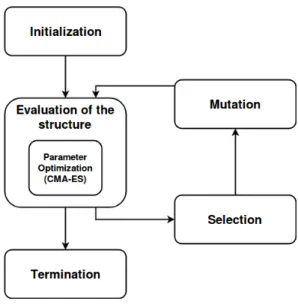
While the structure of the CRN/PIVP defines what is possible, the value of the parameters (i.e. kinetic parameters and initial concentrations) is essential to the function and a bad exploration of the parameter space might lead to a wrong rejection of an actually good structure. To solve this difficulty we use two nested evolutionary algorithms where the first optimizes the structure and the second optimizes the parameter values, as summarized in Fig. 1.
Fig. 1. Schematic representation of the nested evolution algorithm. The initialization corresponds to the creation of different random individuals. The evaluation of a given structure implies a sub-call to the CMA-ES algorithm with a limited time budget, and only the best set of parameters is kept to compute the fitness of the individual in the main algorithm. Elite selection is used where half the population is deleted while the second one is copied, this scheme allows for fast selection (no random number is needed) and keep a constant population size. The mutation scheme incorporates adding or removing variables or monomials, and switching signs. Termination is enforced by fixing the number of generations.
The Covariance Matrix Adaptation Evolution Strategy (CMA-ES) [28] is a black-box derivative-free continuous optimization algorithm used here to opti-mize the kinetic parameters at each step of the CRN structure evolution. This algorithm enjoys many invariance properties with respect to scales as well as linear, rotational or any order-preserving transformations. It is a state-of-the-art algorithm that shows best performances on the hardest non-convex even discontinuous problems [27]. Here the parameters are positive and are searched according to a logarithmic scale. CMA-ES has been used in Biocham for param-eter search and robustness optimization with respect to quantitative temporal logic properties [22,40,39] with notable success in both systems biology [30] and synthetic biology [13] as well as external control of cell processes [44].
Algorithm 1 Structure Optimization
function Evolution(f) population ← InitializePopulation(f) for g in generation do for p in population do StructureFitness(f,p) end for pop_new ← Select(population)
population ← pop_new + Mutate(pop_new) . Concatenate the two lists end for
return Select_best(population) end function
Algorithm 2 Parameter Optimization
procedure StructureFitness(f, pivp) u ← Random(0, 1) if u == 1 then x0 ← RandomInitialState(pivp) else x0 ← InitialStateFromBest(pivp) end if
fit_value, fit_param ← CmaEs(FitnessFunction(pivp),x0) UpdateBestParameters(pivp, fit_value, fit_param) end procedure
The top-level genetic algorithm for learning the structure of the PIVP is given in Alg. 1. Each monomial has a sign, + or -. To handle the constraint of positivity of the concentration variables, a monomial in the ODE of one variable cannot have a negative sign if the variable is not present in the monomial. For example, the derivative of x can depend on −xy but not on −y which is equivalent to
Algorithm 3 Fitness function for functions of time
function FitnessFunction(f, pivp, param) coeff, y0 ← ParamToCoeff(param) sol ← Integrate(pivp, coeff, y0) return Loss(sol, f)
end function
Algorithm 4 Fitness function for functions of input
function FitnessFunction(f, pivp, param) coeff, y0 ← ParamToCoeff(param) value ← 0
for xiin x do
sol ← Integrate(pivp, coeff, y0(xi))
value ← value + Loss(sol, fi)
end for
return value / len(x) end function
say that a degradation reaction must have the degraded species as reactant. This constraint ensures the positivity of the system (Prop. 1 in [21]). With this provision, there exists a canonical (yet not unique) way of associating a CRN to a PIVP, by associating a possibly catalyzed synthesis reaction to each positive monomial, with mass action law kinetics with the monomial coefficient as rate constant, and similarly a degradation reaction to a negative monomial.
The population of possible solutions is initialized with random PIVPs. The number of variables is chosen in a given range with a uniform distribution. They have 1 or 2 monomials per variable with the same probability.
To evaluate the fitness score of a given structure we rely on CMA-ES to find a set of optimized kinetic parameters and initial concentration (Alg. 2). As CMA-ES is a stochastic algorithm and its result may vary from one call to another even for the same structure, only the best parameter set found so far is used to affect the score (that is we do not allow the fitness to decrease). To keep the computation time tractable, CMA-ES is called with a time limit (of the order of the minute depending on the problem at hand). This also mean that, even with a proper initialization of the CMA-ES seed, the result of this optimization may vary according to the current state of the processor. However limiting the number of function evaluations may drastically slow down the algorithm as large PIVP are difficult to integrate.
As for selection, an elitist strategy is applied: the 50% best polynomials are kept and then mutated. It is worth noting that this criterion is only based on the ranking of the individual solutions according to their evaluation and is thus robust with respect to the precise fitness definition.
Several types of mutations are used :
Adding a monomial with a coefficient exp(v) where v is sampled according to the normal law N (0, 1).
Removing a monomial Note that if a variable has no more monomials, a random monomial is added to this variable (thus avoiding an empty ODE). Adding a variable to avoid empty variable, two monomials are added with co-efficients sampled as just explained, and the initial concentration is sampled with the same law.
Removing a variable all the monomials of this variable are deleted too. Restarting That is replacing the PIVP by a new random one having the same
number of variables and 1 or 2 monomials per variable (also called a restart, this enables the exploration of the search space)
At each generation, one of the mechanisms above can happen. The probability of adding or removing a monomial is 0.35. While the other mutations have a probability of 0.1. Moreover, at each generation, the sign of a monomial is changed (if it satisfies the positivity constraint). This high rate of mutation is tempered by the fact that only one half of the population is mutated while the other half is kept unchanged, thus ensuring that the best structures will never be lost through the mutation operator. Hence the term of elitist selection. During the mutation, the good parameters found during evaluation are kept. Note that no cross-overs are implemented in our mutation operator.
After a fixed number of generations, the best structure of the population is selected as the final result and CMA-ES is called a last time with an extended time limit to fine tuned the parameters.
3.2 Parallel Implementation
The previous algorithm has been implemented in Python 3.6.3 using the CMA-ES package cma, the numerical integrator LSODA of the scipy library, and the parallelization package mpi4py [16].
In our evolutionary algorithm, the most time consuming part is the evaluation part since it requires numerical integration to compare the simulation trace to the objective trace. However, since the evaluations of the different individuals in the population are independent, they can be parallelized. Furthermore, since our algorithm uses two nested evolutionary algorithms, it can benefit from two sources of parallelism. For each of them, we can achieve a linear speedup in the number of processors.
The first layer of parallelism is easy to implement, as there is a function Scatter that takes a list from a root process and scatter it to all processes. The function Gather can perform the inverse operation. Adding the second layer is more difficult, especially in our case where it is not possible to transform the two layers into one layer. To overcome this challenge, using the function Split, new communicators are created. There are as many new communicators as individ-uals in the population. At each generation, the population is scattered between the different groups of processes. Each group is dedicated to one individual. Each group performs the evaluation of the individual. The population of CMA-ES is set here to 10 individual parameter sets. In a group, during the evaluation part of CMA-ES, each individual of CMA-ES is thus evaluated by a different process, through a scatter/gather mechanism.
4
Evolved CRN for Mathematical Functions
4.1 Functions of Time
In all this section, we use as fitness function the mean square error between our goal and the simulation trace evaluated on a finite set of time points.
Cosine. Interestingly, the algorithm evolves PIVPs that can be reduced to the following CRN of 3 species and 7 reactions4:
962*A*B for A =[B]=> _. present(A, 1). 4.78*C for _ =[C]=> A. present(B, 0.0028). 544*A*B for B =[A]=> _. present(C, 0.539). 0.477*B for _ =[B]=> B.
1.5 for _ => B.
0.648*B for _ =[B]=> C. 0.346*C for C => _.
On a trace of two periods, the obtained fitness value is L2(A, cos) = 0.042.
This is an excellent fit comparable to the fitness value of L2(fp, cos) = 0.039
obtained with the numerical method (Ex. 1) with a fast parameter set to 100. In this CRN, the positive and negative parts of the cosine are the species A and B. It is worth noticing that these two species are subjected to a fast bi-degradation similar to the encoding of signed variables with two variables for the positive and negative parts shown in Ex. 1. However, this CRN uses the two parts in a non symmetric fashion that makes it unreachable for our compiler.
The oscillatory behavior of this CRN is the limit cycle of the ODE and is reached for a large space of initial conditions. We can also gather together the reactions that have similar monomials (reactions 1 and 3 for example) and even if this affect the precise fit of the cosine, we check that the oscillatory behavior is preserved.
Heaviside. The Heaviside function
Θ(t) = (
0 if t < 0.5,
1 if t ≥ 0.5. (1) is a discontinuous (hence non-computable) function that cannot be defined by a PIVP. Because it is an ideal step function, it is interesting to see what CRN can emerge to best approximate that function. It takes nearly 10 times more generations to evolve a good approximation for Heaviside than it takes to evolve the cosine function. The best result found, with a fitness φ = L2(A, Θ) = 0.0078,
is of the following form:
4
The evolved CRN of this section are available at https://lifeware.inria.fr/wiki/ Main/Software#CMSB19b
1.05e-4*C*C for _ =[C+C]=> A. present(B, 0.993). 1.79*C*C for _ =[C+C]=> B. present(C, 1.14). 3.07*C*C for _ =[C+C]=> C.
1*A*B for _ =[A+B]=> C. 1.38*B*C for C =[B]=> _.
To understand the dynamics of this CRN, we see that the amplitude of the output species is tuned by the parameter of the first reaction. The fourth reaction (_ =[A+B]=> C) is actually unessential to the function even if it can result in a better approximation, its suppression does not significantly modify the trace. The core of the CRN is thus on the competition between species B and C, both starting at low concentration and increasing abruptly around the desired threshold. There, the last reaction imposes a slow-down that makes C disappear and B stabilize. The species of interest A is then only a linear scaling of B to respect the constraints imposed by the fitness function.
It is worth remarking that this solution is surprisingly close to the PIVP method to transform a function of time in a function of input by multiplying each monomial by a variable that decreases exponentially fast, hence halting the computation on the desired state [20]. Here an exploding variable is halted in its course to simulate non-linearity.
Another way our artificial evolutionary algorithm manages to produce Heav-iside like functions is through the generation of sigmoidal functions. The CRN below
k*A*B for B =[A]=> A. present(A, C0). present(B, 1.0).
satisfies the relation C0 ' exp(−k2) in order to have the jump around one half,
and k large makes the jump as sharp as possible. Practically, this make the initial concentration of A vanishingly small.
This mechanism may have several variants depending on the evolutionary history followed by the algorithm. A common one is to implement the sigmoid function through two species with large concentration in order to produce a sharp exponential and to report the output on a third one that is a linear rescaling of a previous one as is the case in the previous example.
4.2 Functions of Input Variables
In this section, the performance of a CRN is measured by recording only the final value of its output species and using a mean square error as global loss function. Here, final value mean the value at a predefined time (t = 1), to ensure that this correspond to the steady state, the norm of the derivative is used as a
penalty. Note that the choice t = 1 has nothing particular as the time may be rescaled.
Cosine. The PIVP structure that commonly emerges by artificial evolution is the following one:
da dt = −2.9 · 10 2· a − 1.8 · 10−1· c (2) db dt = −2.2 · 10 9 · ac − 4.2 · 10−10· c (3) dc dt = 3.8 · 10 −5· ab − 1.0 · 100· c2 (4)
We choose to start from the PIVP to emphasize the importance of neutral trans-formation in the final result of our EA. Here, both time 2.9 · 102t → t and the last variable 7.7 · 106c → c can be rescaled, giving:
da dt = −a − 8.1 · 10 −11· c (5) db dt = −ac − 1.9 · 10 −19· c (6) dc dt = ab − 4.5 · 10 −10· c2 (7)
where all the variable are of the order of unity. The final term in c may safely be ignored and this let us with the same PIVP as the one feed to our compiler to generate the cosine of input:
da dt = −a (8) db dt = −ac (9) dc dt = ab (10)
Here again, a plays the role of a halting species and b and c compute the cosine and sine functions that are halted on the desired value.
Sum of two inputs. The purpose here is to find a CRN to implement the sum function f (x, y) = x + y, as a first example of a case with two inputs. The best solution found by evolution is:
k1*A*A for A =[A]=> B. present(A, input1). k2*A*A for _ =[A+A]=> C. present(B, input2). k2*B*B for _ =[B+B]=> C. present(C, 1.44). k2*A*B for _ =[A+B]=> 2C.
where we have labeled with the same name the rate constants found nearly equal by artificial evolution. On the other hand the values of k1 and k2 do not play any role. Actually, k1 may even be chosen to be null, highlighting a symmetry of the fitness function. The rest of the reaction implements the equation: ˙c = (a + b)2− c2, where the square enforces a faster dynamics and thus
a better convergence.
The general idea is however to balance the positive and negative monomials of variable c to stabilize it on the desired result. A direct consequence of this mechanism is that the initial concentration of C has no importance in the final output. While a human engineer would thus fixed it to 0, our evolutionary algo-rithm proposes a random value. We may however suspect that this is the mean of the output used to train our CRN as such a choice would accelerate the mean convergence time and decrease the final error.
That mechanism may be more clear if written without the squaring: k1*A for _ =[A]=> C. present(A, input1). k2*B for _ =[B]=> C. present(B, input2). k3*C for C => _.
Interestingly, this also gives a generalization where different values for the rates allow us to compute the function:
f [k1, k2, k3](x, y) = k1 k3 x + k2 k3 y. (11)
Several remarks should be done on this CRN. First, it provides a CRN to com-pute online since a modification of the concentration of the input will be trans-mitted to the output. This online CRN algorithm will have the form of an ex-ponential decay with a time rate k1
3. A fast dynamics (high k3) means that
either the output is small, or the energetic cost will be high. Finally, it is known from the study of such process that on the stochastic regime, the distribution of species C will follow a Poisson distribution with a variance equal to its mean. In comparison, the solution found by our EA converges faster and present a higher signal to noise ratio in stochastic semantics.
Heaviside. When considered as a function of input, the non-linearity of the Heaviside function is no longer an issue as it can be computed with continuous function such as a bi-stable switch. For example, starting from the simplest bistable PIVP dadt = a(1 − a)(2a − 1), our compiler generates the following PIVP: 3*A*A for _ =[A+A]=> A. present(A,input).
A for A => _. present(B,input2). 2*A*B for A =[B]=> _.
6*A*B for _ =[A+B]=> B. 4*B*B for B =[B]=> _. 2*B for B => _.
where input2 have to be the square of input. Interestingly, this switch CRN is an instance of the Approximate Majority distributed algorithm extensively studied and related to cell division cycle progression models in [7].
Another solution would be to activate a production and degradation cycle based on the remainder of the input after a fast comparison to a predefined threshold:
fast*A*C for A+C => _. present(A,input). A for _ =[A]=> B. present(C,0.5). A*B for B =[A]=> _.
The best CRN found by evolution in our experiments is however very different from these two solutions, and plays upon the dynamics of the network and the precise point of evaluation defined by the input trace to fit, here at time t = 1. The CRN found displays a transient state of variable length τtwhere the output
is near zero, and a single steady state where the output is near unity. The value of the input impacts the time to reach the steady state so that if the input is greater than one half then τt < 1 and the output is near 1 at evaluation time,
while in the other case, τt> 1 and at the evaluation time t = 1 the output is
null but just temporarily. This illustrates the typical problem of generalization in machine learning for an input/output function specified by a finite trace.
5
Comparison to Natural CRNs in BioModels
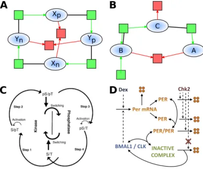
One first remark illustrated by the previous examples, is that when we usually end up with parameters value taking involved values it is often possible, by clever variable transformation, to recover more natural values thus highlighting several symmetries of our fitness function. This is typically the case when evolving the cosine function, the scale of the sine function is undefined and creates a whole va-riety of solutions that are strictly equivalent up to a rescaling of two parameters. This kind of symmetry of the fitness function is one of the plague of biology as it is often difficult to identify them and they may obfuscate a simpler design [26]. A second discussion may be raised by the two CRN for the cosine function of time obtained respectively by the numerical method and the artificial evolu-tion algorithm. Fig. 2 shows that those CRN can be compared to the circadian clocks present in eukaryote and prokaryote albeit with strong differences in their implementations. In prokaryotes, a circadian clock has been shown to be imple-mented through a cycle of phosphorylation and dephosphorylation, such as of the two sites S and T of a KaiC protein polymer found in cyanobacteria[35]. This mechanism is usually presented through a four step process:
ST → SpT → pSpT → pST → ST
where a p preceding a letter indicates that the corresponding site is phosphory-lated. This mechanism is similar to the compiled version of our cosine function where 4 species activates one another in a circular fashion :
where the upper signs denote the positive and negative part of the function.
Fig. 2. Representation of our compiled (panel A) and evolved (panel B) CRN as reac-tion graphs for the cosine funcreac-tion of time. Ellipses represent species, squares indicate reactions in green for productions and red for degradations. Catalysts are linked to their reactions with a bold black line. Panel C shows the molecular oscillator of cyanobac-teria as described in[35]. Panel D shows the genetic oscillator of mammal (similar in most eukaryotes) as proposed in [32].
The eukaryotes use a transcriptional mechanism where a CLOCK protein activates the transcription of its own inhibitor. The action of the inhibitor is however delayed through several steps that may vary from one organism to an-other. Usually this involves translation, dimerization and transportation to and from the nucleus. By using the graph matching method based on subgraph epi-morphism (SEPI) [24] to compare our evolved CRN to models of the BioModels repository, we found a mapping from the mammalian circadian clock models such as [32] toward the simple oscillator in panel B of Fig. 2 presented above. The SEPI mapping makes B play the role of the transcription factor that acti-vates the transcription of the messenger RNA C that then became the protein A that will bind to the transcription factor to form an inactive complex, thus inhibiting the transcription.
Table 1 shows general SEPI comparison results with models in BioMod-els [10]. We see that modBioMod-els presenting oscillations (circadian clock and cell cycle) are far more likely to exhibit a SEPI toward one of our evolved network than the MAPK models (the SEPIs found come from model 026 [36] and 010 [34]). The
Model type Nb. of models Nb. SEPI matchings (min/mean/max) % SEPI Circadian clock 13 3/7.8/12 60% Cell cycle 22 6/10.1/17 45%
Mapk 9 0/0.7/2 08%
Table 1. SEPI matchings from biological models in BioModels having between 5 and 15 species to the 10 best evolved CRNs (over 60 runs) for the cosine time function.
evolved model that harbors nearly all SEPI from both cell cycle and circadian clock models is the one with the best fit presented in section 4.1.
These connections between the result of our evolutionary algorithm and the actual mechanisms found in biology suggest a form of evolutionary convergence. It is well known in biology that organs in species that have evolved totally inde-pendently may in fact be similar. There might be actually few ways to implement a clock that are easily found by evolution so much that every solution that ap-pears is actually a close repetition from the existing one. This kind of evolution convergence has already been emphasized in the case of the evolution of a bi-ological logarithm were every successful run displays the same core mechanism [31]. This provides a tool to decipher the function and constraints of a biochem-ical network by comparing it to an idealized mathematbiochem-ical framework while still being able to make relevant connection with the biological case.
6
Conclusion
We have described a nested evolution algorithm to learn both the structure and the kinetic parameters of a CRN for approximating a function given by a finite trace of either time points for a function of time, or input values.
On a Heaviside function of time, the results obtained by artificial evolution lead to a remarkably simple CRN of 3 molecular species and 5 reactions with double catalysts which provide a very stiff transition although using mass action law kinetics. This solution is more economical than the CRN generated by the PIVP method for sigmoid functions [20]. On a Heaviside function of input, the CRN found by evolution are slightly more complicated than the bistable switch found in cell cycle CRN for instance, but much less complex than the MAPK signaling network that plays a similar role [34].
On the cosine function of time, the best CRN found by evolution contains an annihilation reaction similar to the CRN generated by the numerical method for positive and negative variables, but one less reaction thanks to an intriguing non symmetric use of the two variables which preserves the limit cycle. Interestingly, the evolved and the PIVP generated structures could be compared to prokaryote and eukaryote models of the circadian clock found in BioModels.
On the cosine function of input, a CRN surprisingly emerges with the struc-ture of the CRN for cosine function of time, using the same trick as in [20] to stop time at the desired input value.
These results are encouraging to further develop artificial evolution meth-ods for CRN design in both perspectives of systems biology with the study of evolution convergence, and synthetic biology in addition to rational design.
Acknowledgment: This work benefited from support from the ANR-MOST project BIOPSY “Biochemical Programming System”ANR-16-CE18-0029 and granted access to HPC resources with GENCI allocation 2018-AP011010715.
References
1. Batt, G., Yordanov, B., Weiss, R., Belta, C.: Robustness analysis and tuning of synthetic gene networks. Bioinformatics 23(18), 2415–2422 (2007)
2. Benenson, Y., Adar, R., Paz-Elizur, T., Livneh, Z., Shapiro, E.: DNA molecule provides a computing machine with both data and fuel. Proceedings of the National Academy of Sciences 100(5), 2191–2196 (2003)
3. Bournez, O., Graça, D.S., Pouly, A.: Polynomial Time corresponds to Solutions of Polynomial Ordinary Differential Equations of Polynomial Length. In: 43rd Inter-national Colloquium on Automata, Languages, and Programming, ICALP 2016, July 11-15, 2016, Rome, Italy. LIPIcs, vol. 55, pp. 109:1–109:15. Schloss Dagstuhl - Leibniz-Zentrum fuer Informatik (2016)
4. Cao, H., Kang, L., Chen, Y., Yu, J.: Evolutionary modeling of systems of ordi-nary differential equations with genetic programming. Genetic Programming and Evolvable Machines 1(4), 309–337 (2000)
5. Cao, H., Romero-Campero, F.J., Heeb, S., Cámara, M., Krasnogor, N.: Evolving cell models for systems and synthetic biology. Systems and Synthetic Biology 4(1), 55–84 (3 2010)
6. Cardelli, L., Češka, M., Fränzle, M., Kwiatkowska, M., Laurenti, L., Paoletti, N., Whitby, M.: Syntax-guided optimal synthesis for chemical reaction networks. In: International Conference on Computer Aided Verification. pp. 375–395. Springer (2017)
7. Cardelli, L., Csikász-Nagy, A.: The cell cycle switch computes approximate major-ity. Scientific Reports 2 (09 2012)
8. Cardelli, L., Kwiatkowska, M., Whitby, M.: Chemical Reaction Network Designs for Asynchronous Logic Circuits, pp. 67–81. Springer International Publishing (2016) 9. Carothers, D.C., Parker, G.E., Sochacki, J.S., Warne, P.G.: Some properties of solutions to polynomial systems of differential equations. Electronic Journal of Differential Equations 2005(40), 1–17 (2005)
10. Chelliah, V., Laibe, C., Novère, N.: Biomodels database: A repository of mathe-matical models of biological processes. In: Schneider, M.V. (ed.) In Silico Systems Biology, Methods in Molecular Biology, vol. 1021, pp. 189–199. Humana Press (2013)
11. Chen, Y., Dalchau, N., Srinivas, N., Phillips, A., Cardelli, L., Soloveichik, D., Seelig, G.: Programmable chemical controllers made from DNA. Nature Nanotechnology 8, 755–762 (Sep 2013)
12. Chen, Y., Smolke, C.D.: From DNA to targeted therrapeutics: bringing synthetic biology moving to the clinic. Sci. Transl. Med. 3(106) (Oct 2011)
13. Courbet, A., Amar, P., Fages, F., Renard, E., Molina, F.: Computer-aided bio-chemical programming of synthetic microreactors as diagnostic devices. Molecular Systems Biology 14(4) (2018)
14. Courbet, A., Molina, F., Amar, P.: Computing with synthetic protocells. Acta Biotheoretica 63(3) (Sep 2015)
15. Dalchau, N., Murphy, N., Petersen, R., Yordanov, B.: Synthesizing and tuning chemical reaction networks with specified behaviours. In: International Workshop on DNA-Based Computers. pp. 16–33. Springer (2015)
16. Dalcin, L.D., Paz, R.R., Kler, P.A., Cosimo, A.: Parallel distributed computing using Python. Advances in Water Resources 34(9), 1124–1139 (9 2011)
17. Daniel, R., Rubens, J.R., Sarpeshkar, R., Lu, T.K.: Synthetic analog computation in living cells. Nature 497(7451), 619–623 (05 2013)
18. Dinh, H.Q., Aubert, N., Noman, N., Fujii, T., Rondelez, Y., Iba, H.: An Effective Method for Evolving Reaction Networks in Synthetic Biochemical Systems. IEEE Transactions on Evolutionary Computation 19(3), 374–386 (6 2015)
19. Duportet, X., Wroblewska, L., Guye, P., Li, Y., Eyquem, J., Rieders, J., Batt, G., Weiss, R.: A platform for rapid prototyping of synthetic gene networks in mammalian cells. Nucleic Acids Research 42(21) (2014)
20. Fages, F., Le Guludec, G., Bournez, O., Pouly, A.: Strong Turing Completeness of Continuous Chemical Reaction Networks and Compilation of Mixed Analog-Digital Programs. In: CMSB’17: Proceedings of the fiveteen international conference on Computational Methods in Systems Biology. Lecture Notes in Computer Science, vol. 10545, pp. 108–127. Springer-Verlag (Sep 2017)
21. Fages, F., Gay, S., Soliman, S.: Inferring reaction systems from ordinary differential equations. Theoretical Computer Science 599, 64–78 (Sep 2015)
22. Fages, F., Soliman, S.: On robustness computation and optimization in biocham-4. In: CMSB’18: Proceedings of the sixteenth international conference on Compu-tational Methods in Systems Biology. Lecture Notes in BioInformatics, Springer-Verlag (Sep 2018)
23. Gay, S., Fages, F., Martinez, T., Soliman, S., Solnon, C.: On the subgraph epimor-phism problem. Discrete Applied Mathematics 162, 214–228 (Jan 2014)
24. Gay, S., Soliman, S., Fages, F.: A graphical method for reducing and relating models in systems biology. Bioinformatics 26(18), i575–i581 (2010), special issue ECCB’10
25. Gomez, H.F., Hucka, M., Keating, S.M., Nudelman, G., Iber, D., Sealfon, S.C.: Moccasin: converting matlab ode models to sbml. Bioinformatics 21(12), 1905– 1906 (2016)
26. Gutenkunst, R.N., Waterfall, J.J., Casey, F.P., Brown, K.S., Myers, C.R., Sethna, J.P.: Universally sloppy parameter sensitivities in systems biology models. PLOS Computational Biology 3(10), 1–8 (10 2007)
27. Hansen, N., Auger, A., Ros, R., Finck, S., Pošík, P.: Comparing results of 31 algo-rithms from the black-box optimization benchmarking BBOB-2009. In: Proceed-ings of the 12th annual conference comp on Genetic and evolutionary computation - GECCO ’10. p. 1689. ACM Press, New York, New York, USA (2010)
28. Hansen, N., Ostermeier, A.: Completely derandomized self-adaptation in evolution strategies. Evolutionary Computation 9(2), 159–195 (2001)
29. Hárs, V., Tóth, J.: On the inverse problem of reaction kinetics. In: Farkas, M. (ed.) Colloquia Mathematica Societatis János Bolyai. Qualitative Theory of Differential Equations, vol. 30, pp. 363–379 (1979)
30. Heitzler, D., Durand, G., Gallay, N., Rizk, A., Ahn, S., Kim, J., Violin, J.D., Dupuy, L., Gauthier, C., Piketty, V., Crépieux, P., Poupon, A., Clément, F., Fages, F., Lefkowitz, R.J., Reiter, E.: Competing G protein-coupled receptor kinases balance G protein and β-arrestin signaling. Molecular Systems Biology 8(590) (Jun 2012)
31. Hemery, M., François, P.: In silico evolution of biochemical log-response. The Jour-nal of Physical Chemistry B (2019)
32. Hong, C.I., Zámborszky, J., Csikasz-Nagy, A.: Minimum criteria for dna damage-induced phase advances in circadian rhythms. PLoS Computational Biology 5(5), e1000384 (May 2009)
33. Hsiao, Y.T., Lee, W.P.: Reverse engineering gene regulatory networks: Coupling an optimization algorithm with a parameter identification technique. BMC Bioin-formatics 15(Suppl 15), S8 (12 2014)
34. Huang, C.Y., Ferrell, J.E.: Ultrasensitivity in the mitogen-activated protein kinase cascade. PNAS 93(19), 10078–10083 (Sep 1996)
35. Kageyama, H., Nishiwaki, T., Nakajima, M., Iwasaki, H., Oyama, T., Kondo, T.: Cyanobacterial circadian pacemaker: Kai protein complex dynamics in the kaic phosphorylation cycle in vitro. Molecular Cell 23(2), 161–171 (2006)
36. Markevich, N.I., Hoek, J.B., Kholodenko, B.N.: Signaling switches and bistability arising from multisite phosphorylation in protein kinase cascades. Journal of Cell Biology 164(3), 353–359 (Feb 2004)
37. Oishi, K., Klavins, E.: Biomolecular implementation of linear i/o systems. IET SYstems Biology 5(4), 252–260 (2011)
38. Qian, L., Soloveichik, D., Winfree, E.: Efficient turing-universal computation with DNA polymers. In: Proc. DNA Computing and Molecular Programming. LNCS, vol. 6518, pp. 123–140. Springer-Verlag (2011)
39. Rizk, A., Batt, G., Fages, F., Soliman, S.: A general computational method for robustness analysis with applications to synthetic gene networks. Bioinformatics 12(25), il69–il78 (Jun 2009)
40. Rizk, A., Batt, G., Fages, F., Soliman, S.: Continuous valuations of temporal logic specifications with applications to parameter optimization and robustness mea-sures. Theoretical Computer Science 412(26), 2827–2839 (2011)
41. Rubens, J.R., Selvaggio, G., Lu, T.K.: Synthetic mixed-signal computation in living cells. Nature Communications 7 (06 2016)
42. Sarpeshkar, R.: Analog synthetic biology. Philosophical Transactions of the Royal Society of London A: Mathematical, Physical and Engineering Sciences 372(2012) (2014)
43. Sauro, H.M., Kim, K.: Synthetic biology: It’s an analog world. Nature 497(7451), 572–573 (05 2013)
44. Uhlendorf, J., Miermont, A., Delaveau, T., Charvin, G., Fages, F., Bottani, S., Batt, G., Hersen, P.: Long-term model predictive control of gene expression at the population and single-cell levels. Proceedings of the National Academy of Sciences USA 109(35), 14271–14276 (2012)
45. Valiant, L.: Probably Approximately Correct. Basic Books (2013)
46. Vasic, M., Soloveichik, D., Khurshid, S.: CRN++: Molecular programming lan-guage. In: Proc. DNA Computing and Molecular Programming. LNCS, vol. 11145, pp. 1–18. Springer-Verlag (2018)
47. Vecchio, D.D., Abdallah, H., Qian, Y., Collins, J.J.: A blueprint for a synthetic genetic feedback controller to reprogram cell fate. Cell Systems 4, 109–120 (Jan 2017)