Sand-assisted fluidization of large cylindrical and spherical biomass particles: Experiments and simulation

Open Archive TOULOUSE Archive Ouverte (OATAO)

OATAO is an open access repository that collects the work of Toulouse researchers and

makes it freely available over the web where possible.

This is an author-deposited version published in :

http://oatao.univ-toulouse.fr/

Eprints ID : 13348

To link to this article :

DOI:10.1016/j.ces.2014.12.022

URL :

http://dx.doi.org/10.1016/j.ces.2014.12.022

To cite this version :

Fotovat, Farzam and Ansart, Renaud and Hemati, Mehrdji and

Simonin, Olivier and Chaouki, Jamal Sand-assisted fluidization of

large cylindrical and spherical biomass particles: Experiments and

simulation. (2015) Chemical Engineering Science, vol. 126 . pp.

543-559. ISSN 0009-2509

Any correspondance concerning this service should be sent to the repository

administrator:

staff-oatao@listes-diff.inp-toulouse.fr

Sand-assisted fluidization of large cylindrical and spherical biomass

particles: Experiments and simulation

Farzam Fotovat

a

_{, Renaud Ansart}

b,d

_{, Mehrdji Hemati}

b,d

_{, Olivier Simonin}

c,d

_,

Jamal Chaouki

a,n

a_{Department of Chemical Engineering, École Polytechnique de Montréal, Montréal, Que., Canada}

b_{Université de Toulouse; INPT, UPS; LGC, 4 Allée Emile Monso, BP 84234 31432 Toulouse, France}

c_{Université de Toulouse; INPT, UPS; IMFT, 2 Allée du Pr Camille Soula, 31400 Toulouse, France}

d_{CNRS; Fédération de Recherche FERMAT, 31400 Toulouse, France}

H I G H L I G H T S

!The impact of biomass shape factor on the fluidization characteristics is demonstrated. !_{The axial distribution profile of biomass is obtained by RPT, bed freezing and simulation.}

!_{The reliability of the “frozen bed” technique to quantify the mixing state of the bed contents is assessed by RPT.}

!_{The capability of NEPTUNE_CFD software to predict the distribution and velocity profiles of biomass particles is demonstrated.} !The plausible reasons of some discrepancies between the experimental and simulation results are discussed.

Keywords: Biomass processing Fluidization

Radioactive Particle Tracking CFD simulation

Bubbling Mixing

a b s t r a c t

In this study, bubbling fluidization of a sand fluidized bed with different biomass loadings are investigated by means of the experiments and numerical simulation. The radioactive particle tracking (RPT) technique is employed to explore the impact of the particle shape factor on the biomass distribution and velocity profiles when it is fluidized in a 152 mm diameter bed with a 228 mm static height. Using a pair of fiber optic sensors, the bubbling characteristics of these mixtures at the upper half of the dense bed are determined at superficial gas velocities ranging from U¼0.2 m/s to U¼1.0 m/s. The experimental results show that despite cycling with a similar frequency, spherical biomass particles rise faster and sink slower than the cylindrical biomass particles. Furthermore, bubbles are more prone to break in the presence of biomass particles with lower sphericity. In the separate series of experiments, the reliability of the “frozen bed” technique to quantify the axial distribution of biomass particles is assessed by the RPT results. Using NEPTUNE_CFD software, three-dimensional numerical simulations are carried out via an Eulerian n-fluid approach. Validation of the simulation results with the experiments demonstrates that, in general, simulation satisfactorily reproduces the key fluidization and mixing features of biomass particles such as the global and local time-average distribution and velocity profiles.

1. Introduction

Gas–solid fluidized bed reactors have a wide application in chemical industries. In addition, the fluidization technique is also adopted for various physical processes such as coating, drying and separation. In practice, the solid phase of fluidization often

consists of two or more components differing in physical proper-ties, e.g. size, density and shape. Biomass combustors or gasifiers are examples of fluidized bed systems, where the properties of materials involved in fluidization differ remarkably. Biomass particles are usually so light and large that cannot properly be fluidized. Thus, addition of an inert conventional fluidization material such as sand or alumina is vital to assist their fluidization. In view of the significant difference between the size and density of biomass and bed material particles, however, some new com-plexities arise. Occurrence of segregation of the bed material and biomass particles is one of these complications, which negatively

http://dx.doi.org/10.1016/j.ces.2014.12.022

n_{Corresponding author. Tel.: þ1 514 340 4711x4034; fax: þ1 514 340 4159.}

E-mail addresses:fotovat.farzam@polymtl.ca(F. Fotovat),

affects the performance of fluidized bed units in which chemical reactions take place. In case of biomass processing, due to the lower density of biomass compared to bed material, it tends to migrate to the top layers of the bed while the lowermost parts remain almost devoid of it. This trend, known as flotsam behavior, results in heterogeneity of distribution of reaction products as well as non-uniform temperature profile in the bed, which in turn cause decline in the yield of desired products, formation of tar and emergence of cold/hot spots in the bed. It is noteworthy that segregation could favorably be exploited in systems dealing with physical treatments of materials such as fluidized bed separators

or classifiers (Fotovat et al., 2014c; Sekito et al., 2006; Yoshida

et al., 2010). Thus, it is vitally important to gain a detailed insight into segregation phenomena in fluidized beds.

The common experimental method to assess the degree of mixing/segregation in fluidized beds involving dissimilar compo-nents is based on the analysis of the “frozen bed” that will be

described later on (Detournay, 2011; Hemati et al., 1990; Mourad

et al., 1994). This technique, however, is not capable to provide the actual in situ distribution of particles under fluidization condi-tions. Moreover, it is a demanding method due to the stochastic nature of solids mixing in fluidized beds, which makes repetition of experiments necessary in order to obtain reliable average values of the mixing data. Nonetheless, the results may be still distorted during the bed slumping transients for rapid solids mixing rates (Shen et al., 2007). Employing more advanced techniques for exploring the mixing and multiphase flow aspects of biomass fluidization not only provides more accurate quantitative results of mixing state of bed contents but also is helpful to look into the underlying mechanisms. Radioactive particle tracking (RPT) tech-nique is a non-invasive experimental techtech-nique that is based on the principle of tracking the motion of a single particle as a marker

of interest phase in a flow vessel (Roy et al., 2002). Use of this

technique for studying the solid circulation patterns in binary

mixtures was initially introduced by (Larachi et al. (1995a).

Cassanello et al. (1996) adopted this technique to investigate solids mixing in gas–liquid–solid fluidized beds. More recently,

Upadhyay and Roy (2010)employed this method to explore the mixing and hydrodynamic behavior in a bed consisting of equal weight percentages of the same size particles differing in density. Fotovat et al. carried out extensive pressure and voidage analysis as well as several RPT experiments to explore the fluidized behavior and distribution of large biomass particles mixed with

sand (Fotovat et al., 2011; Fotovat, 2014; Fotovat and Chaouki,

2013; Fotovat et al., 2014b).

Gibilaro and Rowe (1974)as well asNaimer et al. (1982)are the pioneers of modeling the axial segregation of binary mixtures in fluidized beds by considering the different mechanisms governing segregation of dissimilar components. In case of biomass

fluidiza-tion, Zarza Baleato (1986) found that Gibilaro and Rowe (GR)

model could successfully predict the global distribution of parti-cles in the bed when the concentration of large biomass partiparti-cles

is low. However, as indicated byOlivieri et al. (2004)this model

may not always reproduce the experimental data properly. In fact, it is difficult to relate the GR model parameters to real values such as fluidizing velocity and particle size. As a consequence, it has limited use beyond indicating trends and comparing the relative

influence of different mechanisms involved (Leaper et al., 2007).

The computational fluid dynamics (CFD) simulations could shed light on the particle-scale phenomena that should be under-stood well for successful scale-up of fluidized bed units. Hence, they play a central role in the future design and operation of

large-scale biomass-fluidized beds (Goldschmidt and Kuipers, 2001).

The two CFD approaches commonly used for exploring the fluidized bed systems are Eulerian–Lagrangian and Eulerian– Eulerian models. In the Lagrangian approach particles are modeled

as discrete elements and the Newtonian equations of motion for each individual particle are solved with inclusion of the effects of particle collisions and forces acting on the particles by the gas. In this approach, the flow of fluid, which is considered as a con-tinuum phase, is described by the local averaged Navier–Stokes equation. Thus, this approach is a coupling of computational fluid dynamics and discrete particle method (CFD–DPM).

In the Eulerian–Eulerian model, the two phases are treated as interpenetrating continua. Since the volume of a phase cannot be occupied by the other phases, as a result, the concept of phasic

volume fractions is considered (Abbasi et al., 2011). These volume

fractions are assumed to be continuous functions of space and time and their sum is equal to one. Conservation equations for each phase are then derived by obtaining a set of equations that have a similar structure for all phases. Multi-fluid model regarded as a continuum– continuum is the most frequently approach used for predicting the

dynamic behavior of fluid–particle systems (Pain et al., 2001).

In the multi-fluid approach, assumptions need to be made concerning the solids rheology where often Newtonian behavior is

assumed in absence of a more detailed knowledge (Chiesa et al.,

2005). Moreover, the kinetic theory of granular flow is employed in

this approach to provide closures for particle stress tensor. In DPM these assumptions do not need to be made since the motion of each single particle is directly calculated while accounting for interactions with other particles and the continuous phase. However, the CFD– DPM simulation has a disadvantage in comparison to the multi-fluid model. The CFD–DPM simulation requires more computational resources and in case of large fluidized beds with millions of particles the computation demands is considerable and, often, limiting. Thus, its application is limited to the lab-scale fluidized bed.

In spite of relatively large number of studies carried out on

mixing/segregation of regular granular materials (Formisani et al.,

2001, 2008; Marzocchella et al., 2000; Nienow et al., 1978; Olivieri et al., 2004; Tanimoto et al., 1980), there has been a little work on the parameters governing the extent of mixing/segregation in fluidized beds involving irregular materials in terms of size,

density or shape (Cui and Grace, 2007).

Yin et al. (2004)modeled co-firing of biomass with natural gas in 10 m long wall-fired burners in which the particle phase equations were formulated in a Lagrangian frame. Instead of the common assumption of the spherical shape of biomass particles, they assumed solid or hollow biomass cylinders. Accordingly, the particle force balance was modified by considering the shape effect on the drag and lift forces. The shape factor-dependent parameters were also considered in the reaction of biomass particles. The simulation results indicated that the shape of the biomass is a key parameter to accurately model the motion and

the reaction of the biomass particles.Deza et al. (2009)validated

the computational simulations of a fluidized bed in a multi-fluid Eulerian–Eulerian framework through X-ray imaging

measure-ments. Like Yin et al. (2004), they affirmed that the

hydrody-namics of the bed is sensitive to the biomass particle sphericity variations; however, the particle-particle coefficient of restitution

does not affect it meaningfully. Lathouwers and Bellan (2001)

extended the multi-fluid approach to model multi particle classes applied to the pyrolysis of biomass in a dense fluidized bed.

Qiaoqun et al. (2005) investigated experimentally the fluidiza-tion behavior of a binary mixture of sand and rice husk particles. They also simulated the experimented systems via a multi-fluid model based on the kinetic theory of granular flow in which transport equations are used for each individual particle phase and momentum exchanges between different particle phases and between particle and gas phases are taken into account. The 2-D numerical simulations could predict the distributions of the mass fraction of rice husk particles and the mean particle diameter of mixtures of sands with various sizes and rice husk particles.

Sharma et al. (2014)realized 2-D and 3-D numerical simulations of Qiaoqun et al. experiments. They also studied the effects of biomass size and density by simulating fluidization of pinewood particles in the biochar bed; however, there was no experimental data for this mixture to be compared with the simulation results. They found that the choice of drag coefficient correlation, particle–wall and particle–particle interaction parameters has a considerable impact on the hydrodynamics of the biomass–biochar mixture.

Gao et al. (2008)presented the experimental and 3-D compu-tational (Euler–Euler) studies on the flow behavior of a gas–solid fluidized bed with disparately sized binary particle mixtures. The simulations results were in reasonable agreement with experi-mental data in terms of bed expansion, bed density and local composition in the top part of the bed. The results showed that the smaller particles were found near the bed surface while the larger particles of same density tended to settle down to the bed bottom. Moreover, the simulations showed that small particles move downward in the wall region and upward in the core.

Bai et al. (2012) studied the segregation of bed species in a cylindrical fluidized bed containing varying volume fractions of ground walnut shell particles and glass beads, both of which belong to Geldart B type particles. A 2-D multi-fluid model based on the kinetic theory of granular flow was chosen to carry out the

simula-tions. Increasing the ratio of biomass at U¼Umfincreased the extent of

segregation. However, the tendency of mixing of biomass and glass beads rose by increasing gas velocity, regardless of the ratio of the two components in the mixture; thus, the extent of segregation in different mixtures became comparable at high superficial gas velocities. Both experimental and computational results showed that small and light particles did not mix well with large and heavy particles, whereas large and light particles mixed well with small and heavy particles.

Fotovat et al. (2014a)used a computational particle fluid dynamics (CPFD) model to simulate the bubbling characteristics of a bed involving some mixtures of sand and biomass with different mixing ratios. The simulation results, which were validated by the experi-ments, could capture the characteristic asymmetric bubble size and bubble velocity distributions; however, depending on the biomass fraction of the mixture, choice of an appropriate computational mesh size was important to attain the more accurate results.

The present study aims at experimental and numerical inves-tigation of sand fluidized beds involving cylindrical and spherical biomass particles. In this regard, the impact of biomass shape on its fluidization behavior and segregation propensity is explored under bubbling conditions. In addition, the ability of a 3-D Eulerian–Eulerian CFD approach to predict the hydrodynamic characteristics of some studied systems is examined by comparing the simulation with corresponding experimental results.

2. Experimental and simulation description 2.1. Details of the RPT and optical sensor experiments

The RPT experiments are carried out in a cylindrical Plexiglas column 152 mm in diameter. Air is injected into the column through 163 holes, 1 mm in diameter, arranged in a triangular pitch on a stainless steel distributor plate. The percentage of open

area of the perforated plate is less than 1. It should be remarked that compared to the commercial biomass combustors or gasifiers, the cross section of the column used in this study is much smaller. Thus, motion and mixing of the bed inventory particles in our column might be different to some extent from those of the industrial units.

The type of material chosen as biomass particles in this study is the birch wood. The cylindrical biomass pellets are obtained by cutting the wood rods into several pieces while the spherical biomass is purchased and used without any treatment. In order to make sure that the active tracer is the representative of all biomass particles, no significant variety in size or shape is considered for each type of biomass. Thus, the biomass particles used in each experiment are nearly identical in size and shape. Nonetheless, in reality, a broad range of biomass particles in terms of size and shape is fed into the thermal processing unit complicating the hydrodynamic and reaction phenomena. In practice, large biomass particles remain for a relatively long period of time at their original size. This period is long enough to establish the mixing pattern of fuel particles before they reach the high temperatures cause thermal fracture. Biomass particles eventually degrade into fine char (in pyrolysis and gasification) or ash (in combustion) and their proportion and properties change depending on their loca-tion in the bed. These devialoca-tions from the practical systems have not been addressed in this work.

The bed material utilized in the RPT experiments is sand whose

particle size ranges from 100 to 1000

μ

m. Properties of materials

used in the present study have been listed inTable 1. The true and

bulk densities are measured with a gas pycnometer (Micromeri-tics, AccuPyc II 1340) and a graduated cylinder, respectively. The volume equivalent diameter of the cylindrical biomass and the diameter of the spherical biomass particles are almost identical ($9 mm). Moreover, very close true densities of these particles makes the shape factor as the sole hydrodynamic parameter that can differentiate their fluidization behavior.

In a previous study it was shown that the onset of fluidization of bed material and biomass particles known as complete

fluidiza-tion velocity (Uff) is usually larger than the minimum fluidization

velocity of the bed material alone, e.g. sand in this study. Uffof

sand–biomass mixtures rises proportional to the biomass fraction

of the mixture (Fotovat et al., 2013). While Umfof pure sand used in

the experiments is Umf,s¼ 0.18 m/s, Uff of the biomass-sand

mixtures increases to 0.44 m/s for the mixture composed of

16 wt% biomass. The Uffvalues of all investigated systems have

been reported inTables 2 and 3.

The predetermined quantities of sand and biomass are mixed together in order to achieve the intended biomass proportion in the bed. The static bed height is set to 228 mm (H/D¼1.5) in all

experiments.Tables 2 and 3report in detail the properties of the

studied mixtures. In order to start from a well-mixed condition, the sand and biomass measures are each equally divided into eight batches. Each batch of sand is mixed with a single batch of biomass. Finally, the content of all mixtures is sequentially added to the fluidization column.

The tracer used for the RPT experiments is fabricated by embedding a tiny amount of a mixture of Scandium oxide and epoxy resin in a hole made in one of the biomass particles so that Table 1

Properties of materials used in this study.

Material Shape Dp(mm) Lp(mm) Sphericity (Dimensionless) ρp(kg/m3) ρb(kg/m3)

Sand Spherical 0.38 – $ 1 2650 1520

Biomass Cylindrical 6.35 12.70 0.874 824 342

the size and density of the final tracer are almost identical to those of the original particle. Such a tracer could successfully mimic the motion of biomass particles while being fluidized. The tracer is then activated in the SLOWPOKE nuclear reactor of École

Poly-technique de Montréal up to an activity of 70

μ

Ci. The produced

isotope46_{Sc emits}

_γ

_{-rays, which are counted by 12 NaI scintillation}

detectors placed around the column. To maximize accuracy of the RPT results, detectors are staggered in a helical form and cover the whole height of the fluidization region. The horizontal distance between the column and detectors is set according to their saturation lengths measured beforehand.

A high speed data acquisition system counts the number of

γ

-rays

detected by each detector. These counts are analyzed later to calculate the coordinates of the tracer. Details of the system calibra-tion and the inverse reconstruccalibra-tion strategy for determining tracer

position can be found elsewhere (Larachi et al., 1995b, 1994). In each

experiment, the location of the tracer is tracked every 10 ms for about 6 h until finally more than two million points are acquired.

Studying the time/ensemble averaged behavior of a large num-ber of particles on the basis of the flow pattern of a single tracer is possible via considering the concept of ergodicity, which implies the time average of one particle is equal to the population average of many particles, if the system is observed for a sufficiently long

period of time (Monin et al., 2007). Accordingly, the

ensemble-averaged concentration (occupancy) profile of the phase of interest can be obtained as follows: initially, the fluidization bed is divided into the imaginary cells of equal size. Then a counter is assigned to each cell whose amount increases whenever the tracer goes into which. The three dimensional concentration profile of the desired component is calculated by dividing the value of each counter by the sum of all cells counters. In order to attain the velocity profile, the instantaneous Eulerian velocity of the tracer is estimated by subtracting the coordinates of two successive position vectors and dividing it by the counting time interval. The resulting velocity is assigned to the center of the sampling compartment, where the midpoint between the two subsequent positions falls. An ensemble-averaged velocity can be directly estimated by summing each velocity component and dividing by the total number of

instanta-neous velocities assigned to the desired compartment (Larachi et al.,

1996). In this way the time-averaged concentration or axial/radial/

azimuthal velocity profile of the phase of interest can also be evaluated for any desired section of the reactor.

RPT experiments are conducted at low and high superficial gas

velocity, namely U¼ 0.36 m/s (U/Umf,s¼ 2) for all systems and

U¼0.64 m/s (U/Umf,s¼ 3.6) and U¼0.72 m/s (U/Umf,s¼ 4) for

systems composed of cylindrical and spherical biomass, respec-tively. Two high gas velocities are chosen slightly different because of some technical issues. Since both values are well beyond the

Umf,s, it is presumed that the effect of this slight difference on the

following results is negligible. It is important to note that the velocity range studied is similar to that of fluidized bed gasifier but lower than the superficial gas velocity adopted typically in fluidized bed combustors (1–3 m/s).

In the second series of experiments, bubbling characteristics of the bed are studied by placing two identical reflective optical probes at bed heights of 175 and 200 mm above the distributor. Both vertically aligned probes are inserted horizontally into the axis of the column. The superficial gas velocity of each series of experiments varies from 0.2 to 1.0 m/s. The voidage data are acquired for 180 s at a sampling frequency of 512 Hz through a 16 bit A/D data acquisition board with the help of the Labview

9.0.1s _{program. Thus, 92,160 data points are captured for each}

experimental run. These experiments are performed two times and the corresponding average values are reported in the follow-ing sections. To evaluate the bubble size and velocity distributions, an in-house code is developed following the algorithm introduced byRüdisüli et al. (2012).

The probes used in the experiments were built as thin as possible (3.0 mm diameter tip and 4.7 mm diameter body) so that their

intrusive effect on the local flow field was fairly low (Shabanian and

Chaouki, 2014). Moreover, some measures were taken to minimize any remainder intrusive effect of the probes on the bubble proper-ties. For example, bubble size was calculated from the lower probe stem signal since the signal at the upper probe stem might already be influenced by the lower probe stem. Besides, following the algorithm

developed by Rüdisüli et al. (2012), any other potential effects of

probes on bubble characteristics such as bubble distortion or abrupt change in bubble rise velocity was detected and filtered out to guarantee the reliability of the reported results.

Comparing the radial profiles of time-averaged voidage of a traveling fluidized bed column through invasive and non-invasive

techniques,Dubrawski et al. (2013)observed that the results obtained

using optical fiber probes were generally in satisfactory agreement with those obtained non-invasively by using X-ray computed tomo-graphy (X-ray CT) or radioactive particle tracking (RPT). The measured voidages were also reasonably consistent with cross-sectional averages based on pressure gradients and with overall voidages derived from bed expansion measurements. According to them, the invasive probe techniques can provide voidage measurements with errors less than $ 9% with reference to the non-invasive measurements. Hence, it is believed that the reported results obtained by the optical probes are acceptably accurate and trustworthy.

2.2. Details of the “frozen bed” technique

The “frozen bed” technique is normally used to quantify the solids mixing in gas–solid fluidized beds involving two or more components. Experiments are conducted in a cylindrical Plexiglas column of 1000 mm height and 192 mm internal diameter. Flui-dization is performed with air at ambient temperature. At the bottom of the column, a perforated plate provides a homogeneous gas distribution in the bed.

As depicted inFig. 1, bed material and biomass particles are fed

into the bed as several separate layers on top of each other in order to reach initial well-mixed condition (a). The mixture is then fluidized at U¼0.64 m/s (b) and after 20 min the gas flow is quickly cut off (c). Using some metal sheets, the bed is then sectioned off into some strata each one 50 mm in height (d). The bed content is emptied in a section-wise manner (e)–(h) and sieved in order to separate biomass and bed material particles which are finally weighed.

Table 2

Properties of sand-cylindrical biomass mixtures. Wt% of biomass Vol% of biomass Bulk density of sand–biomass mixture Uff (m/s) Voidage of the fixed bed Mass of sand used (kg) Mass of biomass used (kg) 2 6.2 1460 0.24 0.42 5.94 0.12 8 21.9 1350 0.35 0.40 5.12 0.45 16 38.0 1220 0.44 0.37 4.26 0.81 Table 3

Properties of sand–spherical biomass mixtures. Wt% of biomass Vol% of biomass Bulk density of sand–biomass mixture Uff (m/s) Voidage of the fixed bed Mass of sand used (kg) Mass of biomass used (kg) 2 7.7 1530 0.25 0.39 6.18 0.13 8 26.4 1350 0.36 0.36 5.15 0.45 16 43.9 1180 0.49 0.33 4.11 0.78

The biomass used in these experiments is the same cylindrical particles described above; however, the bed material used is

spherical glass beads (

ρ

p¼ 2500 kg/m3, dp¼ 500 mm). As detailed

inTable 4, three mixtures composed of 2 wt.%, 8 wt.%, and 16 wt.% biomass are studied through the frozen bed method. These mixtures correspond to those explored by the RPT technique. 2.3. Details of 3-D numerical simulations

Three-dimensional numerical simulations are carried out using NEPTUNE_CFD. This Eulerian n-fluid unstructured parallelized mul-tiphase flow software is developed in the framework of the NEPTUNE project financially supported by CEA (Commissariat a l'Energie Atomique), EDF (Electricité de France), IRSN (Institut de

Radioprotection et de Sureté Nucléaire), and AREVA-NP (Méchitoua

et al., 2003). The modeling approach for poly-dispersed fluid– particle flows is implemented by Institut de Mécanique des Fluides

de Toulouse (IMFT) (Neau et al., 2013).

The Eulerian n-fluid approach used is a hybrid approach (Morioka and Nakajima, 1987) where the transport equations are derived by phase ensemble averaging for the continuous phase and by using kinetic theory of granular flows supplemented by fluid and turbulent effects for the dispersed phase thanks to joint fluid–particle probability density function (PDF) approach.

In the proposed modeling approach, transport equations (mass, momentum and fluctuating kinetic energy) are solved for each phase and coupled through inter-phase transfer terms. The momen-tum transfer between gas and particle phases is modeled using the drag law of Wen and Yu limited by Ergun equation for the dense

flows (Gobin et al., 2003; Peirano et al., 2002). The collisional

particle stress tensor is derived in the frame of the kinetic theory of

granular media (Boelle et al., 1995). The fluid turbulence modeling

is achieved by the two equations of k–

ε

model extended to

particle-laden flows accounting for additional source terms due to the

inter-phase interactions (Vermorel et al., 2003). For the dispersed phase,

a coupled transport equation system is solved on particle

fluctuat-ing kinetic energy and fluid–particle fluctuatfluctuat-ing covariance (qp2–qfp).

The effects of the particle-particle contact force in the very dense zone of the flow are taken into account in the particle stress tensor

by the additional frictional stress tensor (Srivastava and Sundaresan,

2003). The interaction modeling of particle species approach is

developed in the frame of simulation of reacting gas–solid

poly-dispersed reactive fluidized beds (Batrak et al., 2005; Gourdel et al.,

1999). (detailed inAppendix A)

The 3-D mesh is a column of 600 mm height and 152 mm composed of 178,035 hexahedron, based on O-grid technique with

approximately

Δ

r¼ 3.1 mm and

Δ

z¼4.5 mm (Fig. 2). The

numer-ical simulations are performed on parallel computers with 16 cores. At the bottom (z¼0), the fluidization grid is an inlet for the gas with an imposed uniform superficial velocity corresponding to the fluidization velocity and a wall for the particles. At the top of the fluidized bed, a free outlet for both gas and particles is defined. The wall-type boundary condition is friction for the gas and a

no-slip one for the particles (Fede et al., 2009).

The numerical simulation is divided into two steps: a transitory step of 50 s to let the mixing of biomass–sand be steady and an established regime during which the statistics are computed for

100 s. Favre

α

-weighted averaging is realized by making the

con-tinuity equation exact and eliminating double correlations involving

density fluctuations from the turbulent fluxes (Favre, 1969).

The flow is composed of three phases: gas, media particles (sand) and biomass particles. The phase properties are

summar-ized inTable 5. The particles of each solid phase are assumed to be

spherical with a monodisperse sauter mean diameter. Two differ-ent cases are simulated corresponding to mixtures composed of

8 wt% and 16 wt% biomass fluidized at U/Umf,s¼ 4.

Fig. 1. Schematic presentation of the “frozen bed” technique. Table 4

Properties of sand–cylindrical biomass mixtures studied by the “frozen bed” technique.

Wt% of biomass

Vol% of biomass

Mass of glass bead (kg)

Mass of cylindrical biomass used (kg)

2 7.34 8.52 0.17

8 25.24 8.00 0.69

16 42.51 7.30 1.39

Fig. 2. 3-D mesh for the numerical simulation with 178,035 cells. Table 5

Properties of simulated fluidization phases.

Gas density ρg(kg m% 3) 1.18

Gas viscosity μg(Pa s) 1.85 & 10% 5

Sand particle diameter ds(μm) 380

Sand particle density ρs(kg m% 3) 2650

Biomass particle diameter dB

(mm)

9.52

Biomass particle density ρB

(kg m% 3₎

3. Results and discussion

3.1. Comparing fluidization of cylindrical and spherical biomass particles

It is well known that bubble characteristics feature the fluidi-zation quality and govern gas and solid mixing circumstances in a

bubbling fluidized bed.Fotovat et al. (2013)have shown that the

presence of large cylindrical biomass pellets in a bed of sand gives rise to bubble breakage, thereby the mean bubble size in a sand fluidized bed involving biomass is smaller than that of a bed of

pure sand.Fig. 3 demonstrates the percentage change of mean

bubble size in beds containing cylindrical and spherical biomass with reference to a bed composed of sand alone. The percentage change of mean bubble size is defined as the ratio of the difference between the mean bubble size of pure sand and sand-biomass mixtures to that of pure sand multiplied by 100.The mean bubble size percentage change is calculated on the basis of the values obtained from the optical sensor measurements. As illustrated, the size of bubbles declines by increasing the proportion of biomass, regardless of shape of biomass. However, in case of the cylindrical biomass the percentage change is higher in respect of the corresponding mixtures involving spherical biomass. In other words, bubble breakage is intensified by lowering the biomass particle sphericity. Since the rise velocity of bubbles is propor-tional to the bubble size, it is expected that bubbles rise faster in

the presence of the spherical biomass compared with the cylind-rical biomass. It is noteworthy that while the extent of mean bubble size reduction is almost independent of superficial gas velocity for spherical biomass, it increases monotonously by rising gas velocity when the biomass shape is cylindrical.

In fluidized beds, gross circulation, i.e. upward movement of solids as a consequence of bubble rise and their offsetting down-ward flow in the dense phase, is the main mechanism of the axial distribution of solids along the bed. Accordingly, these are the properties of gross cycles that determine the mixing/segregation propensity of the system. Comparison of gross circulation char-acteristics reveals that the cycle frequency, i.e. number of gross cycles per a given period of time, is comparable for systems containing cylindrical and spherical biomass. This means that the mean cycle time is almost identical for cylindrical and spherical biomass particles. It is true for all corresponding systems in terms of mixture composition or fluidization velocity. In spite of this similarity, the rising and sinking velocities of biomass particles

vary with the shape of biomass. As shown inFig. 4, compared to

the cylindrical biomass, spherical particles rise faster but sink slower when they are involved in gross circulation.

In view of the above discussion, the higher rising velocity is linked to the comparatively larger bubbles in beds containing spherical biomass that rise faster in the bed and induce higher rise velocity of solids. On the other hand, the slower sink velocity of spherical biomass particles can be explained in light of the force

U (m/s) 0.2 0.4 0.6 0.8 1.0 P e rc e n ta g e c h a n g e -60 -40 -20 0 20 2% wt. biomass 8% wt. biomass 16% wt. biomass U (m/s) 0.2 0.4 0.6 0.8 1.0 P e rc e n ta g e c h a n g e -60 -40 -20 0 20 2% wt. biomass 8% wt. biomass 16% wt. biomass

Fig. 3. Percentage change of mean bubble size vs. superficial gas velocity for sand fluidized beds involving different loads of (a) spherical and (b) cylindrical biomass particles with reference to a bed of pure sand (h¼ 175 mm, r/R¼0).

Biomass weight percentage (%)

2 4 6 8 10 12 14 16 Velocity (m/s) -0.3 -0.2 -0.1 0.0 0.1 0.2 0.3

Mean rising velocity (Cylindrical) Mean rising velocity (Spherical) Mean sinking velocity (Cylindrical) Mean sinking velocity (Spherical)

Biomass weight percentage (%)

2 4 6 8 10 12 14 16 Velocity (m/s) -0.4 -0.2 0.0 0.2 0.4

Mean rising velocity (Cylindircal) Mean rising velocity (Spherical) Mean sinking velocity (Cylindrical) Mean sinking velocity (Spherical)

Fig. 4. Mean rising and sinking velocities of the biomass particle involved in gross circulation for systems fluidized at (a) U/Umf,s¼ 2 and (b) U/Umf,s¼ 3.6 for cylindrical and

balance. It is believed that the large cylindrical objects immersed

in a bed of small-heavy particles prefer to sink lengthwise (Rios

et al., 1986). On this basis, the drag force exerted on a sinking cylindrical biomass is smaller than that of a spherical one, because of its smaller cross sectional area. As a consequence, it sinks relatively faster. It should be noted that in order to offset the higher mean upward velocity, the mean downward velocity of spherical biomass particles is higher than that of cylindrical ones, no matter if they have been involved in gross circulation or not.

The difference between the corresponding mean values of rising and sinking velocities of cylindrical and spherical biomass in spite of the similarity of their mean cycle times implies that the time that biomass particle spends in upward or downward paths depends on the particle sphericity. The slower sinking velocity of the spherical biomass is equivalent to the longer time that it resides in the emulsion phase against that of a cylindrical biomass. The larger residence time in the emulsion phase matters from the practical point of view since it is more likely that the products of biomass devolatilization are released into the interstitial gas of the emulsion phase rather than into the bubbles, which bypass the bed. This could result in higher performance of the biomass processing unit due to the more uniform distribution of gas reaction products in the bed.

The axial distribution of biomass particles in the bed is investi-gated through the “frozen bed” and RPT techniques. For this purpose, in the “frozen bed” experiments the dense bed is axially divided into 5 slices, each one is 50 mm in height. To introduce the effect of the

bed expansion on the results shown in Fig. 5, the representative

height of each slide, i.e. the middle point height, is multiplied by the

expansion factor of the bed, i.e. (H/H0). H and H0are the expanded

and the initial height of the dense bed, respectively, which are the average of readings of three graduated measuring tapes attached to the outer wall of the column. The normalized mass of biomass in ith

slice (mi,N) is then calculated based on Eq.(1)

mi;N¼

mB;i

MB ð1Þ

where mB,iand MBare the mass of biomass in slice i and the entire

bed, respectively.

For the RPT tests, the lowermost 500 mm of the bed including both dense bed and splash zone is virtually sliced into 10 layers

again 50 mm in height. To determine mi,Nin this approach, the

ratio of occurrence of tracer in slice i to the total number of occurrences is multiplied by the total mass of biomass.

Fig. 5 exhibits the axial profile of the normalized mass of

biomass as obtained from both experimental techniques. mi,N

increases by rising in the bed denoting the flotsam behavior of

biomass. On the basis of the RPT results, mi,Nsharply diminishes

above the dense bed height under the fluidization conditions. With reference to the in situ distribution of biomass demonstrated by the RPT results, the higher degree of the bed expansion is, the more significant error arises in the results of the “frozen bed” technique. Since the extent of the bed expansion decreases by increasing the load of biomass, the “frozen bed” method is more reliable when the load of biomass is greater in the bed.

Fig. 5also shows that the axial distribution of cylindrical and spherical biomass is comparable, particularly when the biomass load is low. By raising the biomass fraction in the bed, cylindrical biomass particles display a stronger tendency to migrate to the top layers of the dense bed. Nonetheless, it is comparatively less likely to find cylindrical biomass particles in the splash zone. It signifies that with reference to the spherical biomass particles, cylindrical ones are less liable to accompany the rising bubbles in the bed.

To compare quantitatively the mixedness degree of the studied systems, a mixing index is introduced and calculated on the basis of the RPT data. In this regard, the bed volume is cut into the

several slices. The ratio of occurrence of the tracer in a given slice to the total number of occurrences multiplied by the total volume of biomass particles provides the biomass volume in that slice. The ratio of biomass volume in ith slice to the slice volume gives the

local volume fraction of biomass in slice i (XB,iin Eq.(2)).

Ii¼ XB;i XB;total ð2Þ MIvol¼ 1 % XB;total PN i ¼ 1ðIi% 1Þ2 N 1 % X" B;total# !1=2 ð3Þ

Normalized mass of biomass (-)

0.0 0.1 0.2 0.3 0.4 Height (cm) 0 10 20 30 40 50 RPT (Cylindrical) RPT (Spherical) Frozen bed

Normalized mass of biomass (-)

0.0 0.1 0.2 0.3 0.4 Height (cm) 0 10 20 30 40 50 RPT (Cylindrical) RPT (Spherical) Frozen bed

Normalized mass of biomass (-)

0.0 0.1 0.2 0.3 0.4 Height (cm) 0 10 20 30 40 50 RPT (Cylindrical) RPT (Spherical) Frozen bed

Fig. 5. Axial profile of the normalized mass of biomass as obtained by the RPT and

frozen bed techniques for mixtures fluidized at U/Umf,s¼ 3.6 for cylindrical and

U/Umf,s¼ 4 for spherical biomass particles, which are composed of (a) 2 wt% (b) 8 wt

where XB,total,and N are the total volume fraction of biomass and

the total number of slices in the bed, respectively.

In this study the volume based mixing index was preferred over the mass based one, because in the absence of the occupancy profile of the bed material, calculation of the mass based mixing index requires evaluation of the bed voidage and bubble phase fraction along the bed. Estimation of these parameters is merely possible by using some correlations, which could result in redu-cing the accuracy of the mass based mixing indices.

Fig. 6exhibits the trend of mixing index evolution by changing the shape and load of biomass as well as the superficial gas velocity. At low portion of biomass (2 wt%), the mixing indices of all systems are highly comparable, regardless of the fluidization velocity. Increasing the biomass load in the bed gives rise to a decline in the mixing index. Raising fluidization velocity improves the mixing state of the biomass and sand particles; however the extent of enhancement of mixing depends on the shape of biomass. In case of cylindrical biomass increasing gas velocity boosts mixing up to a fixed level independent of the mixture composition. For mixtures composed of spherical biomass this effect is correlated to the portion of biomass in the bed. In other words, the larger is the portion of spherical biomass in the bed, the higher is the positive effect of increasing gas velocity on the mixing. This is attributed to the lower chance of bubble breakage in the presence of spherical biomass, which results in more vigorous bubbling behavior of the bed that renders the axial biomass distribution more uniform. As

seen in Fig. 6, this could offset the unfavorable impact of the

higher loads of biomass on the mixing index of the systems involving spherical biomass.

3.2. Bubbling characteristics of the studied systems: experimental vs. simulation results

Characterization of bubbles as the “mixing agents” is vitally important to understand the phenomena controlling the degree of mixing/segregation in bubbling fluidized beds involving dissimilar components. Moreover, experimental validation of the properties of the bubbles obtained from simulation implies the capability of the model to successfully predict the underlying mechanisms of mixing/ segregation. In this study, the simulated voidage signals were obtained at the same positions, where the voidage was recorded experimentally using the optical probes (r/R¼0, h¼175 mm and h¼200 mm). The same post-processing method that was applied to the experimental voidage signals was also employed to analyze the signals coming from simulation.

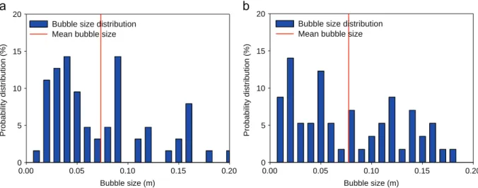
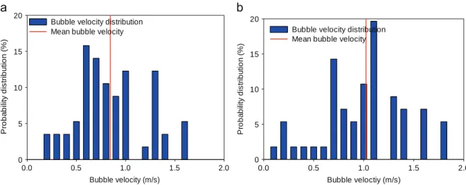
Figs. 7 and 8 respectively compare the size and velocity distributions of bubbles detected in the experiments and simula-tions for the system composed of 8 wt% spherical biomass and

fluidized at U/Umf,s¼ 4. The overall profiles are closely comparable

for both bubble size and velocity distributions. The mean size and velocity of the bubble detected in simulations are respectively 0.08 m and 1.00 m/s, which are very close to the corresponding experimental values, i.e. 0.07 m and 1.03 m/s.

Ub¼ U % Umf

"

# þ0:711 gdð bÞ0:5 ð4Þ

Velocity of each detected bubble vs. its size has been exhibited in Fig. 9 for both experimental and simulation approaches. As

reported previously (Fotovat et al., 2013), the theoretical

David-son–Harrison correlation (Eq. (4)) generally overestimates the

trend of the bubble velocity vs. bubble size for the bubbles obtained from the experiment because the effect of biomass on the bubble break-up is not considered in this correlation. On the other hand it satisfactorily follows the trend of bubbles detected in simulation denoting that bubble properties have been preserved and look like those of a bed of a pure sand, which is not in agreement with the experimental observations.

Like Figs. 7 and 8, the experimental and simulation mean

values shown inFig. 9are very comparable; however, the

scatter-ing patterns of data are different. It signifies that the mean bubble size/velocity of the systems differing in composition is not enough

Biomass weight percentage (%)

2 4 6 8 10 12 14 16 MI vol (-) 0.70 0.75 0.80 0.85 0.90 0.95 1.00

Spherical biomass ( U/Umf,s=2)

Spherical biomass ( U/Umf,s=4)

Cylindrical biomass ( U/Umf,s=2)

Cylindrical biomass ( U/Umf,s=3.6)

Fig. 6. Volume-based mixing index of the studied systems.

Bubble size (m) 0.00 0.05 0.10 0.15 0.20 Probability distribution (%) 0 5 10 15 20

Bubble size distribution Mean bubble size

Bubble size (m) 0.00 0.05 0.10 0.15 0.20 Probability distribution (%) 0 5 10 15 20

Bubble size distribution Mean bubble size

Fig. 7. Comparison of (a) experimentally measured and (b) numerically calculated bubble size distribution for the mixture composed of 8 wt%. spherical biomass particles

(U/Umf,s¼ 4, r/R ¼ 0, h ¼ 175 mm). Red lines indicate the mean value of the bubble size (For interpretation of the references to color in thisfigure legend, the reader is referred

to compare their bubbling behavior. In this work, the mean values are simply obtained by averaging size or velocity of all bubbles detected in experiments or simulation.

Comparison of the experiment and simulation results for the bubbles in the mixture composed of 16% biomass shows that the above-mentioned facts are also true for this system.

3.3. Time-average distribution and velocity profiles of biomass particles: experimental vs. simulation results

Fig. 10shows the normalized time-averaged concentration (occu-pancy) contour and 2-D velocity vector plot of the spherical biomass particles in the mixture composed of 8 wt% biomass. Both profiles are obtained non-invasively by the RPT method. For this purpose, the bed space is compartmentalized by means of azimuthal slices of several radial and axial cuts. The ratio of occurrence of the tracer in a specific compartment to the total number of occurrences, i.e. total fraction of recorded instantaneous positions, is considered as the corresponding normalized concentration of that compartment. An ensemble-averaged velocity can also be directly evaluated by aver-aging the velocity components assigned to each compartment as explained in detail in the experimental section.

Fig. 11portrays the time-average volume fraction and the stream-line of the biomass particles in the above system as obtained from

simulation. It should be noted that despite the difference in defini-tion, the volume fraction corresponds to the normalized concentra-tion so that these parameters can analogously represent the distribution of biomass particles in the bed. Comparison of corre-sponding experimental and simulation figures denotes that simula-tion can truly predict the flotsam behavior of biomass particles; however, in contrast to the experimental result, the lateral locus of the biomass accumulation is predicted much closer to the bed wall.

In accordance with the experimental velocity vector plot,Fig. 11

shows that a rotating toroidal vortex is formed along the bed. Indeed, it is known that the bubbles near the wall tend to move away from the walls due to coalescence with the neighboring bubbles. This bubble behavior renders the ascent of biomass particles at the center of the bed, which is offset by their descent at the wall region; a fact that is confirmed by both experimental and simulation plots.

As seen in Figs. 10 and 11, a significant portion of biomass

particles accumulates at the wall proximity in the column used in this study; however, this portion is much smaller when biomass is fluidized in a large industrial bed, where the biomass particle size is much smaller than the bed diameter and the wall effects are negligible. In other words, much less relative concentration of biomass is expected close to the wall in actual fluidized bed combustors or gasifiers, since rise and sink of solid particles takes place in several solids mixing cells rather than only a single cell Bubble velocity (m/s) 0.0 0.5 1.0 1.5 2.0 P ro b a b ili ty d is tr ib u ti o n ( % ) 0 5 10 15 20

Bubble velocity distribution Mean bubble velocity

Bubble veloctiy (m/s) 0.0 0.5 1.0 1.5 2.0 P ro b a b ili ty d is tr ib u ti o n ( % ) 0 5 10 15 20

Bubble velocity distribution Mean bubble velocity

Fig. 8. Comparison of (a) experimentally measured and (b) numerically calculated bubble velocity distribution for the mixture composed of 8 wt% spherical biomass

particles (U/Umf,s¼ 4, r/R ¼ 0, h ¼ 175 mm). Red lines indicate the mean value of the bubble velocity (For interpretation of the references to color in thisfigure legend, the

reader is referred to the web version of this article.)

Bubble size (m) 0.00 0.05 0.10 0.15 0.20 Bubble velocity (m/s) 0.0 0.5 1.0 1.5 2.0 2.5 3.0 Detected bubbles

Davidson and Harrison equation (Eq. 4) Mean value Bubble size (m) 0.00 0.05 0.10 0.15 0.20 Bubble velocity (m/s) 0.0 0.5 1.0 1.5 2.0 2.5 3.0 Detected bubbles

Davidson and Harrison equation (Eq. 4) Mean value

Fig. 9. The rise velocity of all detected bubbles vs. the respective sizes for the mixture composed of 8 wt% spherical biomass particles as obtained from (a) experiments and

(b) simulation (U/Umf,s¼ 4, r/R ¼ 0, h ¼ 175 mm). Full black dots denote the mean bubble rise velocity vs. the mean bubble size. The solid curve represents the Davidson and

observed in small columns like ours (Olsson et al., 2012). Note that

the vortex shown inFigs. 10 and 11is indeed the half section of the

solids mixing cell since each cell consists of two adjacent vortices. It has been reported that the larger concentration of biomass at the wall region results in the emergence of the smaller bubbles

and the lower dense phase fraction (Fotovat et al., 2014b). This

effect is less likely in large fluidized beds involving biomass in view of the discussion above. This conclusion is in agreement with

the experimental observations ofFarzaneh et al. (2013).

Another important effect of increasing the bed size on the hydrodynamics of fuel particles is remarkable rise in their lateral

solids dispersion coefficient (Liu and Chen, 2010). The higher the

lateral solids dispersion coefficient, the better distribution of fuel particles is achieved over the cross section of the bed.

It should be noted that in order to be able to demonstrate the time-average concentration and velocity profiles of a 3-D bed in 2-D plots, the respective values should be azimuthally averaged.

Therefore, the values shown inFigs. 10, 11 and 13–15are indeed

the azimuthal-average of the corresponding parameters.

As depicted in the Fig. 12obtained from the RPT results, the

experimental time-averaged concentration and velocity profiles of the studied systems were fairly axisymmetric, thus the profiles demonstrated for the half part of the column adequately represent the trend of concentration and velocity changes along the bed for Fig. 10. (a) Time-average concentration (occupancy) and (b) velocity profile of the biomass particles in the bed as obtained from the RPT experiments. (biomass fraction: 8 wt%,

U/Umf,s¼ 4).

Fig. 11. (a) Time-average volume fraction and (b) streamline of the biomass particles in the bed as obtained from the numerical simulation. (biomass fraction: 8 wt%,

the whole bed. Uniform axisymmetric fluidization observed in the

experiments is consistent with the findings ofDrake and Heindel

(2011, 2012). By using X-ray computed tomography (CT) and analyzing the local time-averaged gas holdup at 12 azimuthal

locations for glass beads and crushed walnut shell (dp¼ 500–

600

μ

m), they realized that fluidization was uniform in their 3-D

15.2 diameter column. In addition, they found that when the bed aspect ratio is greater than 0.25 (H/D4 0.25) fluidization is axisymmetric. It is the criterion met in our tests (H/D¼1.5) implying the axisymmetry of fluidization.

3.4. Biomass particle velocity: experimental vs. simulation results The time-average radial profile of the vertical component of the

biomass velocity is shown inFig. 13for six different heights above the

distributor. As mentioned above and seen inFig. 13, particles rise in the

core of the bed and sink in the bed annulus. It is noteworthy that as

imposed by the boundary conditions in the numerical simulations biomass velocity is practically close to zero at the wall proximity.

Numerical simulations predict a monotonous increase in par-ticle velocity by rising up to the bed surface in the central region of the column; however, the RPT data show a decrease in this velocity by rising beyond h¼20 cm. This phenomenon can be attributed to the bubble breakage due to the accumulation of large biomass particles at the top of the bed. Consequently, a lower bubble and biomass rise velocity is expected at the top layers of the bed. A plausible reason for occurrence of a local minimum in the experimentally obtained radial profile of the axial velocity of biomass is as follows. Indeed, the biomass particles studied in this work are too large to be displaced in the wake of bubbles and it is

believed that they mainly exist in the emulsion phase (Fotovat

et al., 2014b). Accordingly, in view of the dominance of bubbles at the center of the bed, it is unlikely that biomass particles rise with the emulsion phase in this zone and consequently a decrease in biomass rise velocity is observed by approaching to the center of

Fig. 12. (a) Time-average concentration (occupancy) and (b) velocity profile of the biomass particles in the entire bed as obtained from the RPT experiments. (biomass

fraction: 8 wt%, U/Umf,s¼ 4).

Fig. 13. Comparison between (a) the RPT experimental measurements and (b) the 3-D numerical simulation results for the time-average vertical component of biomass

the bed. It is especially the case at the levels that the bubble activity is remarkable (15 cmoho25 cm).

Numerical predictions and experimental measurements are in relatively good agreement; however, the numerical simulations seem not to be able to predict the decrease in the biomass velocity at the top of the bed due to the biomass accumulation. It is worth pointing out that with reference to the experimental results, simulation could successfully predict the radial location of the zero mean axial velocity or the biomass flow inversion point, which is about r/R¼0.6.

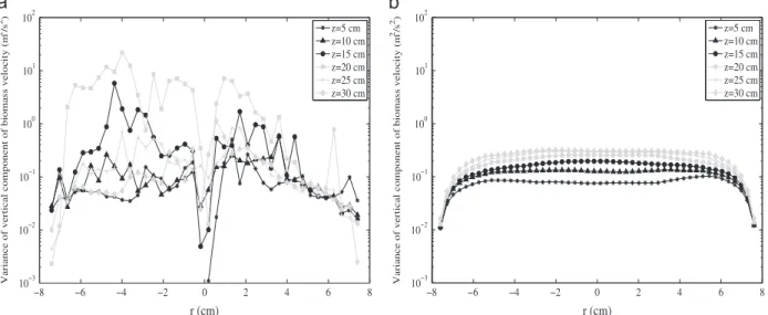
The radial profiles of variance of vertical and radial components of biomass velocity at several heights in the bed are plotted inFigs. 14 and 15, respectively. It can be seen that the corresponding numerical and experimental values have almost the same order of magnitude with a minimum close to the wall region. Moreover, anisotropy of the velocity fluctuations can be observed since the vertical fluctuations are 4 times higher than the radial fluctuations for the numerical simulation and much higher for the experimental data. It is noted that in the vertical direction the numerical results generally underestimate the variance of biomass velocity.

The velocity-related profiles shown inFigs. 13–15 are indeed

the azimuthal-averages of the corresponding parameters when

the tracer traverses the compartments located at a specific height above the distributor (see legend of each figure for the respective heights of the compartments). As indicated earlier, this averaging should be done to drop the azimuthal dependence of the velocity-related profiles and make it possible to exhibit them in a 2-D plot. The numerical radial profiles presented in this section are from

the O–y direction butFig. 16shows that the profiles are

symme-trical in the two perpendicular directions presented. The authors have checked that all time-averaged bed values are axisymmetric. 3.5. Axial biomass segregation: experimental vs. simulation results

Fig. 17presents the time-average axial profile of the normalized mass of biomass for mixtures composed of 8 wt% and 16 wt% biomass. A satisfactory level of consistency is observed between the numerical results and experimental measurements; however, simulation under-estimates the extent of biomass accumulation at the top of the bed, instead, it predicts a more uniform distribution of biomass along the bed. In agreement with the RPT measurements, the simulation results show a slight increase in the normalized mass of biomass at the bottom of the fluidized bed with an increase in the biomass weight

Fig. 14. Comparison between (a) the RPT experimental measurements and (b) the 3-D numerical simulation of the variance of the vertical component of biomass velocity.

(biomass fraction: 8 wt%, U/Umf,s¼ 4).

Fig. 15. Comparison between (a) the RPT experimental measurements and (b) the 3-D numerical simulation of the variance of the horizontal component of biomass velocity.

percentage. On the other hand, simulation seems not able to repro-duce the sharper drop in the biomass content in the freeboard (above the dense bed surface) with increasing the biomass fraction as observed experimentally.

These discrepancies have to be linked to the failure of simulation to predict reduction in the bubble velocity at the top levels of the bed because of the biomass accumulation as discussed above. In fact, due to the high predicted bubble size and velocity at the top of the bed, bubbles are spuriously so energetic that can lift higher quantities of biomass to the freeboard and, as a result, simulation overestimates the mass fraction of biomass in this zone.

3.6. Discussing the plausible reasons of discrepancy between the experimental and simulation results

As discussed above, the numerical simulation approach adopted for this study could successfully predict the key features of sand-assisted biomass fluidization. Nonetheless, some discrepancies were noticed in the profiles of biomass velocity and biomass distribution along the bed. It is believed that the main reason of emergence of

these discrepancies is simulation's incapacity to consider the impact of the large biomass particles on the bubbling characteristics especially at the top half of the bed, where the biomass particles dominate. An evidence for this claim is the higher probabilities of large and fast bubbles obtained from the simulation in comparison with the corresponding experimental results. These bubbles are those that have higher size or velocity than the mean bubble size

or velocity values illustrated inFigs. 7–9.

Additionally, as inferred from the simulated time-average variance of the vertical and horizontal components of biomass

velocity (Figs. 14 and 15), the numerical approach predicts a

monotonous evolution of bubbles as they rise in the bed, while the corresponding experimental results are intensively fluctuating probably because of the interaction between bubbles and biomass particles. This interaction leads to the breakage of the large bubbles as well as a slowdown in the biomass rise velocity.

To improve the simulation approach several tracks can be followed. First of all, the numerical simulations were carried out according to the classical monodisperse drag law. It has been shown in several case studies that the drag law has a significant Fig. 16. (a)Time-averaged and (b) variance of the vertical component of biomass velocity in two perpendicular directions as obtained from the 3-D numerical simulation

(biomass fraction: 8 wt%, U/Umf,s¼ 4).

influence over the qualitative and quantitative nature of the flow

and segregation (Leboreiro et al., 2008a, 2008b). New drag

treat-ment, which has been developed specifically for polydisperse mixtures using Lattice-Boltzmann simulations, may improve the

description of the drag force (Beetstra et al., 2007; Hoef et al.,

2005). However, this bidisperse drag law, which is established for

fixed beds, is only accurate when the size difference between

particles is moderate (Yin and Sundaresan, 2009).Holloway et al.

(2010)combined the fluid–particle drag relation described byYin and Sundaresan (2009)for low Reynolds number flows and that

given byBeetstra et al. (2007)for fixed beds under moderate fluid

inertia and constructed a drag force model that applies to poly-disperse, high Stokes-number and moderate Reynolds number.

The second track is to improve the momentum exchange between particle species. These exchanges are governed by the polydisperse collisions, which are due to the mean particle– particle relative velocity between the solid phases and the particle fluctuating motion represented here by the particle agitation.

From the experimental work point of view, it should be noted that the results may come with some uncertainties. It has been reported that the different sources of noise such as Poisson

statsitcs of the

γ

-ray counts, density fluctuations in the flow and

propagation error through algorithmic computation cause a dis-crepancy between the true tracer location and the tracer position

obtained by RPT (Chaouki et al., 1997). In order to assess the extent

of error in locating the tracer in this study some tests were performed for each experiment by placing the tracer in several

known locations in the bed and measuring the

γ

-ray counts for

twelve hundred times. The average distance between the actual and apparent position of the tracer was less than 4 mm in both axial and radial directions that is acceptably low.

4. Conclusions

Different experimental techniques and an Eulerian n-fluid approach were adopted in this work to shed light on the fluidiza-tion and mixing characteristics of large biomass particles fluidized with sand under the bubbling conditions. By using the fiber optic sensors and the RPT technique, it was noticed that the shape of biomass particles could influence the properties of bubbles and, as a result, the cycling features of the solids in the bed. Formation of relatively smaller bubbles was observed when the shape of biomass changed from sphere to cylinder. As a consequence, the rise velocity of the cylindrical biomass particles was lower than that of the spherical ones. Unlike the mixtures consisted of cylindrical biomass, enhancement of mixing index by increasing gas velocity was correlated to the portion of the spherical biomass in the bed.

Comparison of the axial distributions of the biomass particles revealed that the results of the “frozen bed” technique become less reliable when the bed expansion is considerable, e.g. at high gas velocities or when the biomass fraction is relatively low in the bed. Simulation was successful to reproduce the experimental dis-tribution profiles of bubble size and velocity at h¼175 mm; however, the probability of formation of bubbles that were larger in size or velocity than the corresponding mean values was overestimated with reference to the experimentally detected bubbles. In accordance with the experimental observations, simu-lation predicted much more intense velocity fluctuations of biomass particles in the axial compared to the radial direction. The flotsam behavior of the biomass particles as well as their streamline was properly reproduced by simulation. With Com-pared to the experimental data, simulation predicts a slightly more uniform distribution of biomass in the axial direction. The observed discrepancies between the experimental and simulation results were attributed to the incapacity of the simulation to allow

for the impact of biomass particles on the properties of bubbles, particularly where the biomass accumulation is significant. NomenclatureSymbols

Cd drag coefficient (dimensionless)

H height above the distributor (m)

Ik interphase momentum exchange (kg/m2/s)

MB total mass of biomass (dimensionless)

MIvol volume based mixing index (dimensionless)

N total number of slices in the experiments

(dimensionless)

Pk pressure of phase k (Pa)

Rep particle Reynolds number (dimensionless)

U superficial gas velocity (m/s)

Uk,i mean velocity of phase k (m/s)

Vd,i drift velocity (m/s)

Vrp,i mean relative velocity gas and particle (m/s)

X volume fraction of biomass (dimensionless)

dp particle diameter (m)

ec elasticity coefficient during inter-particle collision

(dimensionless)

g gravitational constant (m/s2₎

g0 particle pair correlation function (dimensionless)

k turbulent kinetic energy (m2_/s2₎

mB,i mass of biomass in ith slice (dimensionless)

mi,N normalized mass of biomass in ith slice (dimensionless)

mp mass of particle p (kg)

np number of particle per volume unit (m% 3)

qfp fluid–particle fluctuating covariance (m2/s2)

qp2 particle fluctuating kinetic energy (m2/s2)

u0

k;i fluctuating velocity of phase k (m/s)

Greek letters

α

k volume fraction of phase k (dimensionless)

ε

turbulent dissipation rate of gas (m2_/s3₎

Σ

k,ij effective stress tensor of phase k (Pa)

ϕ

angle of internal friction rad

μ

k dynamic viscosity of phase k (Pa s)

ρ

k density of phase k (kg/m3)

τ

Fgp mean gas particle relaxation timescale (s)

τ

c

pq particle–particle collision time (s)

τ

tgp interaction time between particle motion and gas

fluctuations (s) Subscripts

B biomass

g gas

i slice index/ith component of a vector

ff full (complete) fluidization

mf minimum fluidization

p,q particle

s sand

Acknowledgments

This experimental work of this study was funded by the Natural Science and Engineering Research Council (NSERC) and TOTAL American Services, Inc. industrial chair. The simulation part was granted due to having access to the HPC resources of CALMIP

under the allocation P11032 and CINES under the allocation gct6938 made by GENCI.

Appendix A

The Eulerian n-fluid approach used is a hybrid approach where the transport equations are derived by phase ensemble averaging for the continuous phase and by using kinetic theory of granular flows supplemented by fluid and turbulent effects for the dis-persed phase thanks to joint fluid–particle probability density function (PDF) approach.

In the following equations, subscript k or m¼g refers to the gas phase and k or m¼p or q to the particle phase.

α

m

ρ

m (m¼p,q) in the particle transport equation represent

nmmm where nmis the number density of m-particle center and

mm is the mass of a single m-particle:

α

m¼ nmmm/

ρ

m is an

approximation of the local volume fraction of particle m.

Hence, gas and particle volume fractions,

α

g,

α

pand

α

qhave to

satisfy

α

gþ

α

pþ

α

q¼ 1 ðA1Þ

A.1. Mass transport equation

∂

∂t

α

k

ρ

kþ

∂

∂x_j

α

k

ρ

kUk;j¼ 0 ðA2Þ

where

ρ

kis density of the k phase and Uk,iis the i-component of its

velocity.

A.2. Momentum transport equation

α

k

ρ

k ∂U_k;i ∂t þ Uk;j ∂U_k;i ∂x_j & ' ¼ %

α

k ∂P_g ∂x_iþ

α

k

ρ

kgiþ X m a k I_m-k;i% ∂P k;ij ∂x_j ðA3Þ

Where Pg is the mean gas pressure and gi is the gravity

i-component. I_g-pand I_g-qare the inter-phase momentum transfer

between particle and gas without the mean gas pressure

con-tribution and Ip-q¼ % Iq-pis the inter-phase momentum transfer

between particle species, and P I_m-k;i is the effective stress

tensor of phase k.

A.3. Interphase transfer modeling

A.3.1. Gas–particle mean momentum transfer

According to the particle to gas density ratio, the dominant forces between the gas phase and p-particles are the drag and Archimede's forces, so the mean momentum gas–particle transfer term may be written

I_g-p;i¼ %

α

p

ρ

p

τ

F gp Vrp;i ðA4Þ 1

τ

F gp ¼3 4

ρ

g

ρ

p 〈j v!rj〉p dp CdðRepÞ ðA5Þ Cd"Rep# ¼ Cd;WY if

α

gZ0:7

min C) d;WY; Cd;Erg* if

α

go0:7

( ðA6Þ Cd"Rep# ¼ 24 Rep 1þ0:15Re 0:687 p ,

-α

% 1:7 g Repo1000 0:44

α

% 1:7 g RepZ1000 8 < : ðA7Þ Cd;Erg¼ 200 1%

α

g " # Rep þ 7 3; Rep¼

α

g

ρ

g〈jv!rj〉pdp

μ

g ðA8Þ

Vrp;i¼ 〈 vr;i〉p¼ Up;i% Ug;i% Vdp;i ðA9Þ

Vdp;i¼ % Dtgp;ij 1

α

p ∂

_α

_p ∂x_j% 1

α

g ∂

_α

_g ∂x_j & ' with Dt gp;ij¼ 1 3

τ

tgpqgp

δ

ij ðA10Þ

Vrp,iis the mean relative velocity written in terms of the mean gas

and p-particle velocities and a turbulent gas–particle drift velocity:

Vdp,i. Vdp,iaccounts for the transport of the p-particles by the gas

turbulent eddies. (Gobin et al., 2003; Simonin et al., 1993) Cd,WY

and Cd,Erg are respectively the Wen and Yu and Ergun drag

coefficients.

A.3.2. q to p-particles mean momentum transfer

FollowingGourdel et al. (1999), the collisions between particles

lead to a mean momentum transfer between classes which can be written I_q-p;i¼ % mpmq mpþ mq 1þec 2 f c

pqH1ð Þ Uz" p;i% Uq;i# ðA11Þ

fc pq¼ g04

π

npnqd2pqgr; dpq¼ d" pþ dq#=2 ðA12Þ np¼

α

p

π

d3_p=6; mp¼

ρ

p

π

d 3 p=6 ðA13Þ g_r¼ ffiffiffiffiffiffiffiffiffiffiffiffiffiffiffiffiffiffiffiffiffiffiffiffiffiffiffiffiffiffiffiffiffiffiffiffiffiffiffi 16

π

2 3q2pqþ Vpq;iVpq;i r

; Vpq;i¼ Up;i% Uq;i; q2pq¼

1 2 q2pþ q2q , -ðA14Þ g0¼ 1 %1%

_α

α

g max & '% 2:5αmax ; if 1%

α

go

α

_max ðA15Þ H1ð Þ ¼z 8þ3z_6þ3z ðA16Þ

A.4. Particle stress modeling

Σ

p;ij¼ Pp%

λ

p ∂U_p;n ∂x_n & '

δ

ij%

μ

p ∂U_p;i ∂x_j þ ∂U_p;j ∂x_i % 2 3 ∂U_p;n ∂x_n

δ

ij & ' ðA17Þ

μ

p¼

α

p

ρ

p

ν

pkinþ

ν

colp þ

ν

f rictp

, -ðA18Þ

ν

kinp ¼ 1 3qgp

τ

tgpþ 1 2

τ

Fgp 2 3q2p"1þ ^

α

pg0

Φ

c# & ' & 1 þ

τ

F gp 2

σ

c ^

τ

cp " #% 1 ðA19Þ

ν

colp ¼ 4 5

α

^pg0ð1þecÞ

ν

kinp þ ^dp ffiffiffiffiffiffiffiffiffi 2 3 q2 p

π

s 2 4 3 5 ðA20Þ

ν

f rictp ¼ Pf sinϕ 2 1 %ð αgÞρp ffiffiffiffiffiffiffiffiffiffiffiffiffiffiffiffiffiffiffiffiffiffiffiffiffiffiffi I2Dþ ð2=3Þðq2 p=d2pÞ p ; Pf¼ Fr 1 %αg ð Þ%αs; min ½ -n αs; max% 1 %ð αgÞ ½ -q; Fr ¼ 0:05;

ϕ

¼

π

4 I2D¼ ∂U_p;i ∂x_j þ ∂U_p;j ∂x_i & _'∂U p;i ∂x_j % 2 3 ∂U_p;i ∂x_i ∂U_p;j ∂x_j ; n ¼ 2; q ¼ 5;

α

s; min¼ 0:6 ðA21Þ

Φ

c¼2 5ð1þecÞ 3eð c% 1Þ;

σ

c¼ 1 5ð1þecÞ 3 % eð cÞ ðA22Þ