HAL Id: hal-02861706
https://hal.univ-lorraine.fr/hal-02861706
Submitted on 9 Jun 2020HAL is a multi-disciplinary open access archive for the deposit and dissemination of sci-entific research documents, whether they are pub-lished or not. The documents may come from teaching and research institutions in France or abroad, or from public or private research centers.
L’archive ouverte pluridisciplinaire HAL, est destinée au dépôt et à la diffusion de documents scientifiques de niveau recherche, publiés ou non, émanant des établissements d’enseignement et de recherche français ou étrangers, des laboratoires publics ou privés.
A Comparative Fluxmetric (CFM) Method for
Apparent Thermal Conductivity Measurement of
Insulating Materials at High Temperature
Yves Jannot, Johann Meulemans, Vincent Schick, Maxime Capp, Isabelle
Bargain
To cite this version:
Yves Jannot, Johann Meulemans, Vincent Schick, Maxime Capp, Isabelle Bargain. A Compara-tive Fluxmetric (CFM) Method for Apparent Thermal Conductivity Measurement of Insulating Ma-terials at High Temperature. International Journal of Thermophysics, Springer Verlag, 2020, 41, �10.1007/s10765-020-02676-x�. �hal-02861706�
1
A Comparative FluxMetric (CFM) method for apparent thermal conductivity
measurement of insulating materials at high temperature
1Y. Jannot1, J. Meulemans2, V. Schick1, M. Capp2,3, I. Bargain1 1 Université de Lorraine, CNRS, LEMTA, F-54000 Nancy, France
2 Saint-Gobain Research Paris, 39 quai Lucien Lefranc, F-93303 Aubervilliers, France 3 Ecole des Mines, 92 Rue Sergent Blandan, 54042 Nancy, France
Abstract This article presents a simple thermal characterization method, noted CFM, for the
measurement of the apparent thermal conductivity of insulating materials at high temperature (i.e., up to 600°C). The CFM method is a steady-state relative measurement method which requires a calibration. The calibration of the experimental apparatus was done with a calcium silicate board of known thermal conductivity. Thermal conductivity measurements were carried out on a low-density compressible fibrous felt and a high-density calcium silicate board between 100 and 600°C. A good agreement was observed with the values obtained with the guarded hot-plate (GHP) method for the low-density fibrous felt and the parallel hot-wire (PHW) method for the high-density calcium silicate board. The measurement of the apparent thermal conductivities of low-density fibrous felts of different apparent densities, combined with a simple conducto-radiative model, allowed to estimate a mean specific extinction coefficient in good agreement with a value derived from transmittance/reflectance measurements.
Keywords Insulating material. High temperature. Thermal conductivity 1 Introduction
Knowledge of the thermal conductivity of insulating materials at high temperature is of great importance for the control of industrial processes. For example, the cooling rate of a liquid metal in a mold (which has a great influence on the mechanical properties of the molding) is highly dependent on the thermal resistance of the surrounding insulation.
Thermal insulation materials are usually porous materials. Their thermal transport properties, at a macroscopic scale, are not intrinsic values since they depend on the local structure of the material (i.e., porosity, tortuosity) [1] and the contributions of several heat transfer modes (i.e., conduction, convection and/or radiation). The term apparent (or effective) thermal conductivity is thus used for porous materials.
The characterization of the thermal transport properties (i.e., thermal conductivity and thermal diffusivity) of materials can be performed with a large variety of methods. The choice of the method depends on the following criteria: the nature of the material, the size and shape of the specimen, the temperature range, the thermal conductivity and thermal diffusivity range, the uncertainty of measurement [2].
1International Journal of Thermophysics (2020) 41:94, https://doi.org/10.1007/s10765-020-02676-x Corresponding author: Y. Jannot, [email protected]
2
The guarded hot-plate (GHP) [3-5] and the heat flow meter (HFM) [6] methods are the most common methods [7] for thermal conductivity measurement of insulating materials. However, the use of the GHP and HFM methods requires specimen of large dimensions (i.e., around 600×600mm2 and 300×300mm2 for the GHP and HFM, respectively). This requirement is not always convenient when investigating the thermal transport properties of new materials (i.e., at the design stage). For measurements at high temperature (i.e., up to 1000 °C), round robin tests carried out between National Metrology Institutes (NMI) such as the “Laboratoire National de Métrologie et d'Essais" (LNE) in France and the National Physical Laboratory (NPL) in UK have shown that significantly higher uncertainties (from the order of 10% to 18%) occur when using the GHP or HFM methods at temperatures from 100 °C up to 600 °C and higher [8, 9]. This might explain why there are currently no Certified Reference Materials (CRM) for thermal insulation materials at high temperatures.
Methods such as the centered-hot plate (CHP) method [10 11], the three-layer (3L) method [12, 13] or the calibrated tiny hot plate (CTHP)method [14] are thus the preferred methods at the design stage of new material because they only need small samples. However, these methods are not suited to high temperature measurements.
The Flash method [15, 16] is not suitable to the thermal diffusivity measurement of insulating materials [2].
The transient plane source (TPS) (or hot disk) [17, 18] method can be used up to 800°C but due to the strain exerted on the sensors, the durability of the mica insulated sensors is limited [19]. Besides, the TPS method is deemed not practical for the characterization of anisotropic (orthotropic) materials since it requires at least two separate experiments:
- A calorimetric experiment to determine the specific heat before carrying out and analyzing a TPS measurement [18].
- Two separate TPS measurements carried out with two different orientations of the hot disk sensor within the sample [20].
The hot-wire (HW) [21, 22] and the parallel hot-wire (PHW) [23, 24] methods allow the measurement of thermal conductivity at high temperatures but only for isotropic materials. Besides, it is well-known that the TPS [25, 26], HW [21] and PHW [24] methods are not accurate for low-density insulating materials.
The state of the art showed that there is currently no experimental method available to characterize the thermal conductivity of (low-density) thermal insulation materials of small sizes, that may be anisotropic, at high temperatures. A novel experimental method for the characterization of the apparent (or effective) thermal conductivity of thermal insulation materials up to approximately 600 °C was thus developed.
The aim of this work is to validate the proposed method through a dedicated experimental study carried out on different thermal insulating materials (i.e., a low-density fibrous felt and a high-density calcium silicate board) which thermal conductivity is deemed well-known.
A second objective is to measure and interpret the apparent thermal conductivity of a low-density fibrous felt as a function of the temperature and its apparent low-density through a simple conducto-radiative model.
2 Principle and model
3
thermal conductivity of thermal insulation materials. Figure 1 represents a schematic overview of the experimental configurations.
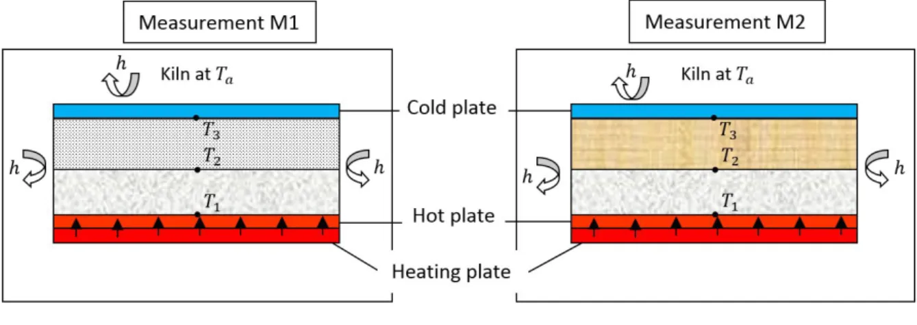
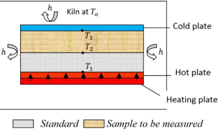
Figure 1: Schematic view of the CFM device
A specimen and a reference material are sandwiched between two metallic plates. A first measurement (Measurement M1) is performed with a specimen which thermal conductivity is well-known (calibration phase). A second measurement (Measurement M2) is then undertaken with a specimen which thermal conductivity is unknown. A heat source is placed at the bottom, below the metallic plate. Three thermocouples are located at the interface between the bottom metallic plate and the reference material ( ), between the specimen and the and the reference material ( ) and between the specimen and the top metallic plate ( ). The metallic plates are needed to ensure a homogeneous temperature on top of the specimen and at the bottom of the reference material. The whole configuration is placed in a kiln. The temperature of the kiln is then adjusted to a temperature .
The CFM method is relative measurement method which requires a calibration with a material (or a set of materials) with known thermal conductivity(ies).
At the initial state, the system is at a uniform temperature (i.e., = = = ). A constant heat source density is then prescribed on the bottom metallic plate. The temperature will thus not be uniform anymore (i.e., ≠ ≠ ). At steady-state, if we assume that the heat transfer is unidirectional at the center and that the contact thermal resistances can be neglected, the thermal resistance of the reference material (Measurement M1) is given by the following formula:
= (1)
where , and are the thermal resistance of the reference material (in m² K W-1), the thickness of the standard material (in m) and the thermal conductivity of the standard material (in W m-1 K-1), respectively.
Conversely, the thermal conductivity of the specimen (Measurement M2) can be determined with the following formula:
4
where and are the thickness of the specimen (in m) and the thermal conductivity of the specimen (in W m-1 K-1), respectively.
The characterization of the thermal conductivity of a specimen is thus a two-step process (measurements M1 and M2). The reference material is used here as a fluxmeter.
An alternative approach is illustrated in Figure 2. This configuration would allow the characterization of the thermal conductivity of a specimen in only one step. However, any difference in the calibration of one of the three thermocouples used would lead to an error in the determination of the thermal conductivity of the specimen. In the chosen configuration, this possible difference is taken into account in the value of the thermal resistance of the reference material without any consequence in the estimation of the thermal conductivity of the specimen.
Figure 2: Schematic view a possible alternative method
3 Measurement device
Figure 3: Views of the device
The experimental setup consists of the following elements (see Figure 3):
- An electric fusing kiln (Enitherm, FC100 model) of internal dimensions 550×550×350 mm3 and controllable temperature up to 1050°C.
- An external mechanical air extraction system to evacuate the potential emissions from the materials.
- An insulation layer (Superwool® HT™ blanket) placed at the bottom of the kiln. - A 300×300×10 mm3 metallic plate (stainless steel 316L) with a 2×2 mm² groove to
insert a 4m long heating wire (Thermocoax Inconel 600).
5
- A 300×300×10 mm3 metallic plate (stainless steel 316L) placed on top of the heating plate in order to ensure a homogeneous temperature on top of the specimen and at the bottom of the reference material. A 0.5×0.5 mm² groove was added in order to insert a sheathed type K thermocouple (diameter 0.5 mm) at the center of the plate (temperature noted in Figure 2).
- A reference material of dimensions 300×300×30 mm3 with known thermal resistance (calcium silicate board LUX500, Final Advanced Materials). A 0.5×0.5 mm² groove was added in order to insert a sheathed type K thermocouple (diameter 0.5 mm) at the center of the top surface of the material (temperature noted in Figure 2).
- A specimen with unknown thermal conductivity is placed on top of the reference material. Its dimensions are either 200×200 mm² or 300×300 mm² with a nominal thickness between 20 and 30 mm. Specimen of dimensions 200×200 mm² are surrounded with four blocks of calcium silicate boards of dimensions 50×250 mm² in order to have a total area of 300×300 mm². For compressible materials, the height of the surrounding frame sets the thickness of the specimen.
- A 300×300×10 mm3 metallic plate (stainless steel 316L) placed on top of the specimen. A 0.5 × 0.5 mm² groove was added in order to insert a sheathed type K thermocouple (diameter 0.5 mm) at the center of the bottom surface of the plate (temperature noted in Figure 2).
- A passive insulating guard made of calcium silicate boards (LUX500, Final Advanced Materials) is placed around the stack.
- The sheathed type K thermocouples are connected to a data logger (Picolog TC-08) in order to record the temperatures with an acquisition rate of 1 s.
- A recorder/controller (Eurotherm nanodac™) allows to record and control the temperature setpoints (kiln and heating plate).
4 Materials and methods
An experimental study was carried out to confirm the theoretical study.
The reference material was a sample of LUX500 (Final Advanced Materials) with a thickness of 30 mm. LUX500 is a calcium silicate based material. Its density, = 770 kg m , was measured by weighing the sample and measuring its dimensions. The values of its thermal conductivity measured by GHP apparatus at LNE [5] are reported in Table 1.
Table 1: Thermal conductivity of LUX500
(°C) 20 200 400 600
(W m-1 K-1) 0.195 0.212 0.210 0.189
The standard material was a sample of SILCAL 1100 (Silca refractory solutions) with a thickness of 30 mm. The thermal conductivity of SILCAL 1100 at various temperatures was measured by several laboratories and the following polynomial fit was established between 300 and 1100 K [27]:
= 0.06797 + 3.699 × 10 + 6.202 × 10 − 8.502 × 10 (3)
Where is the temperature in K.
6
First, the method was validated using two materials with known thermal conductivities: Quartzel felt (Saint-Gobain Quartz) and LUX800 (Final Advanced Materials).
Quartzel felt is made of fused quartz filaments assembled together. The thermal conductivity of Quartzel felt with a density = 26 kg m and a 30 mm-thickness was measured with a guarded hot-plate (GHP) apparatus at LNE between 20°C and 500°C. The values are reported in Table 2.
The measurements of the thermal conductivity of Quartzel felt with the CFM method were carried out with samples having the five following densities: 17, 21, 26, 34 and 42 kg m-3. Their section was 200×200 mm2 and they were surrounded by LUX500 pieces having a 30 mm thickness.
LUX800 is a calcium silicate based material. Its density, measured by weighing the sample and measuring its dimensions, is = 850 kg m . Its thermal conductivity was measured with the parallel hot-wire (PHW) method using the model developed by Jannot and Degiovanni [24]. The values are reported in Table 3. The sample used for the measurements with the CFM method had a 30 mm thickness and a 300×300 mm2 section.
Table 2: Thermal conductivity of a Quartzel felt ( = 26 kg m and = 30 ) measured with guarded hot-plate (GHP) method at LNE
(°C) 20 100 200 300 400 500
(W m-1 K-1) 0.0346 0.0500 0.0803 0.126 0.191 0.273
Table 3: Thermal conductivity of the LUX800 material measured with the parallel hot-wire (PHW) method
(°C) 200 300 400 500 600
(W m-1 K-1) 0.295 0.295 0.291 0.294 0.299
For each sample tested, the temperature of the (bottom) ‘hot’ metallic plate is adjusted to the maximum measurement value desired while that of the (top) ‘cold’ metallic plate is lower than 40°C. For each measurement temperature, the three monitored temperatures reach a stable value before going to a lower measurement temperature.
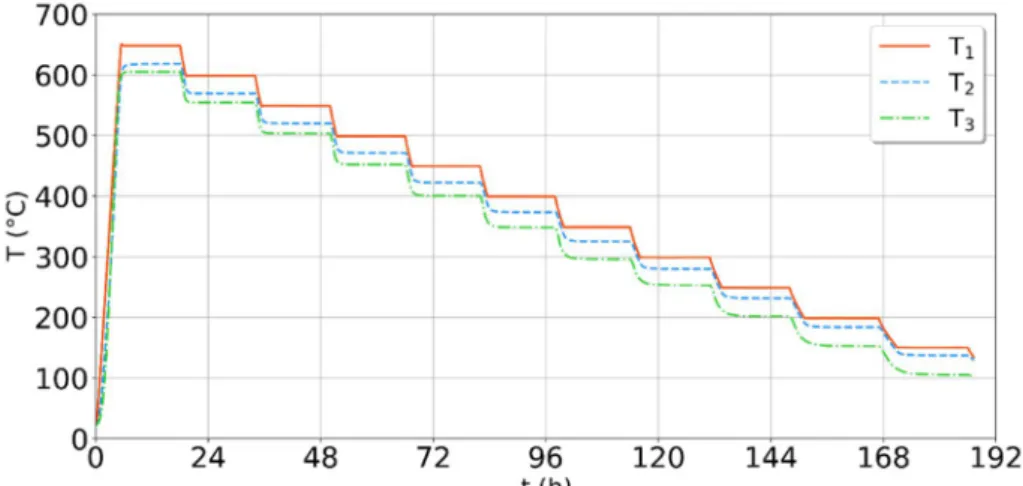
Figure 4: Example of the temperature evolution for a low-density fibrous felt (Quartzel® felt,
7
Figure 4 represents an example of a temperature evolution during a CFM measurement on a low-density fibrous felt (Quartzel® felt, = 26 kg m ). In this example, the measurements were carried out between 600 and 100°C and were completed after 192 hours (8 days).
5 Uncertainty estimation
Calling ( − ) and ( − ) the temperature difference measured during the calibration experiment and combining relations (1) and (2), the estimated value of the thermal conductivity of a sample may be expressed as:
= (( )) (4)
The relative uncertainty on is:
∆ =∆ +∆ +∆ +∆( )
+∆( )+∆(( )) +∆(( )) (5)
The temperatures are measured with the same thermocouples in the two experiments so that if the values of ( − ) and ( − ) on one hand and ( − ) and ( − ) on the other hand are close, then relation (4) shows that the systematic error due to calibration errors of each thermocouple is weak.
Considering the values and the uncertainties of each parameter given in table 4, the relative uncertainty on the estimated value of the thermal conductivity is about 11%. One can note that half of the error is a systematic one due to the uncertainty on the thermal conductivity of the reference sample.
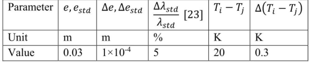
Table 4: Parameters values with their uncertainties
Parameter , ∆ , ∆ ∆
[23] − ∆ −
Unit m m % K K
Value 0.03 1×10⁻⁴ 5 20 0.3
6 Results and discussion
In this section, we will present and discuss measurements carried out on a low-density fibrous felt (Quartzel® felt from Saint-Gobain Quartz, ( = 26 kg m ) and a high-density calcium silicate board (LUX800 from Final Advanced Materials, ( = 850 kg m ). The apparent thermal conductivities measured with standardized methods (i.e., the guarded hot-plate method for the low-density fiber felt and the parallel hot-wire method for the high-density calcium silicate board) will be compared to the values measured with the CFM method.
6.1 Calibration
The first step of the experimental study was to estimate the value of the thermal resistance of the reference sample of LUX 500. The experimental results are presented in table 5. Table 5: Calibration results obtained with a 30 mm thick SILCAL 1100 sample
°C 200 300 400 500 600
8
6.2 Validation
Other measurements have then been realized on a Quartzel® felt sample with a thickness = 30 mm and a density = 26 kg m and on a LUX800 sample with a thickness = 30 mm and a density = 850 kg m .
The results obtained for Quartzel® are reported in figure 5. The apparent thermal conductivity significantly increases with temperature (i.e., a three-fold increase is observed between 150 and 450 °C) as expected for such light-weight fibrous materials.
Two specimen were measured with the CFM method in order to assess the reproducibility of the measurements. The values measured for both specimens were almost identical. The differences between the values obtained with both the GHP and the CFM methods were deemed not significant (i.e., the relative differences were within the uncertainty bounds of the measurement methods).
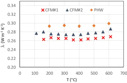
Figure 6 represents the apparent thermal conductivity of the high-density calcium silicate board LUX800 measured with the parallel hot-wire (PHW) method [24] and the CFM method. Concerning the PHW method, 3 measurements were performed for each temperature, reported values are the mean and standard-deviation for each temperature.
The measurements were repeated two times with the CFM method in order to assess their repeatability. The values measured were almost identical. The apparent thermal conductivity is rather constant with the PHW method and the CFM method over the temperature range investigated here. The differences may be explained by the thermal contact resistances on each side of the sample: an air layer thickness of 0.1mm on each side leads to an under-estimation of the thermal conductivity by 8% with the CFM method, that is the order of magnitude of the deviations observed on figure 6. This indicates that the thermal conductivity value = 0.3 W m K can be considered as the measurable upper limit for the CFM method for dense incompressible insulating materials.
Figure 5: Apparent thermal conductivity of a low-density fibrous felt (Quartzel® felt,
( = 26 ) as a function temperature measured by CFM (two measurements series)
and GHP methods 0.00 0.05 0.10 0.15 0.20 0.25 0.30 0.35 0.40 0 100 200 300 400 500 600 (W m -1 K -1) T (°C) CFM #1 CFM #2 GHP
9
Figure 6: Apparent thermal conductivity of a high-density calcium silicate board (LUX800) measured by CFM (two measurements series) and PHW methods
The good agreement observed on the apparent thermal conductivity measurements carried out with standardized methods (GHP and PHW) and the CFM method for different insulating materials (i.e., a low-density fibrous felt and a high-density calcium silicate board) validates thus the CFM method. It also fixed its upper limit to = 0.3 W m K for dense incompressible insulating materials.
6.3 Apparent thermal conductivity of a low-density fibrous felt
The CFM method was used to investigate the influence of the apparent density of Quartzel® felts on their apparent thermal conductivities. Measurements were carried out on samples of dimensions 200×200×30 mm3. The apparent density was adjusted though the mass/weight of the specimen (fixed volume).
Figure 7 shows the apparent thermal conductivities measured for Quartzel® felts with densities of 17, 21, 26, 34 and 42 kg m-3.
Figure 7: Apparent thermal conductivity of Quartzel® felts as a function of temperature for different apparent densities
0.20 0.22 0.24 0.26 0.28 0.30 0.32 0.34 0 100 200 300 400 500 600 700 (W m -1K -1) T (°C) CFM#1 CFM#2 PHW 0.0 0.1 0.2 0.3 0.4 0.5 0.6 0 100 200 300 400 500 600 (W m -1K -1) T (K) 17 kg m-3 21 kg m-3 26 kg m-3 34 kg m-3 42 kg m-3
10
The apparent thermal conductivity decreases when the apparent density increases. This is attributed to a higher contribution of thermal radiation for lower apparent densities (i.e., lower apparent extinction coefficients).
For light-weight fibrous materials, the apparent thermal conductivity can be represented with a parallel model [2] written as follows:
= + + (6)
where:
solid volume fraction (quartz)
thermal conductivity of the solid phase void volume fraction
thermal conductivity of air radiative thermal conductivity
For an optically thick medium (i.e. = ≫ 1 ), the diffusion approximation holds [28] and a thermal “radiative" conductivity can be defined as follows [29]:
= ( ) (7)
Where:
refractive index of the medium
Stefan-Boltzmann constant (in W m-2 K-4) sample thickness (in m)
extinction coefficient of the sample (in m-1) optical thickness of the medium
, emissivities of the walls bounding the medium
3/4 for optically thick media (Deissler approximation) Temperature (in °C)
The density of the bulk material (i.e., quartz) is 2650 kg m-3 so that the void fraction in a Quartzel® felt of apparent density is worth:
= 1 − (8)
For a Quartzel® felt of apparent density of 26 kg m-3, the void fraction = 0.99 and the solid fraction is thus = 0.01.
For the low-density fibrous felts investigated here, the void fraction is greater than 98%, we will thus consider that the refractive index of the medium is the one of air (i.e., = 1).
The thermal conductivity of air between 20°C and 600°C can be calculated with the following formula [30]:
= −3.074 × 10 + 8.171 × 10 + 0.02428 (9)
where is the temperature in °C.
The thermal conductivity of quartz between 0°C and 527°C can be calculated with the following formula [31]:
= 2.996 × 10 − 3.848 × 10 + 2.161 × 10 + 1.303 (10)
where is the temperature in °C.
The thermal conductivity of Quartz exhibits moderate variations (approximately 30% with respect to the mean value over the temperature range investigated here) and the solid volume fraction is smaller than 2% for the low-density fibrous felts investigated here. We can thus
11
consider the thermal conductivity of the solid phase (quartz fibers) as independent of the temperature and write:
= + ( ) + ( ) (11)
We will assume that the medium is grey and that the extinction coefficient can be considered constant, i.e. it does not vary with temperature. The first assumption (grey medium) is consistent with the findings of Maanane et al. [32] based on the estimation of the absorption and scattering coefficients of a Quartzel® felt (with a density = 18.4 kg m ) from transmittance / reflectance measurements carried out at room temperature. The second assumption (invariance of the extinction coefficient with temperature) will be discussed later.
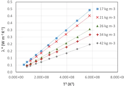
Figure 8 represents the reduced thermal conductivity ( ∗ = − ( )) as a function of (in K3) for different apparent densities. The dashed lines correspond to the (weighted least-squares linear fits). The intercept of the linear fit corresponds to the thermal conductivity of the solid phase ( ). The (mean) extinction coefficient beta can be derived from the slope of the linear fit if both the emissivities and the thickness are known:
= − + − 1 (12)
Here, we will use the following (constant) values for the supposedly known parameters: = 30 ± 0.1 mm and = = 0.9 ± 0.05.
Figure 8: Reduced thermal conductivity ∗ of Quartzel® felts as a function of (in K3) for different apparent densities (empty symbols = measurements, dashed lines = weighted
least-squares linear fits)
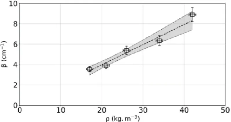
Figure 9 and table 6 present the derived extinction coefficients as a function of the apparent density of the material. The extinction coefficient exhibits a linear variation with the apparent density (the dashed line correspond to the weighted least-squares linear fit). The assumption of the invariance of the extinction coefficient w.r.t. temperature seems valid. It should be noted that the optical thicknesses are greater than 10.6, the media are thus optically thick and the diffusion approximation is valid.
0.0 0.1 0.1 0.2 0.2 0.3 0.3 0.4 0.4 0.5 0.5
0.00E+00 2.00E+08 4.00E+08 6.00E+08 8.00E+08
* (W m -1K -1) T3(K3) 17 kg m-3 21 kg m-3 26 kg m-3 34 kg m-3 42 kg m-3
12
The specific extinction coefficient, noted = (in m2 kg-1), can be calculated and is worth 19.7 m2 kg-1 ± 11.3%. This value is consistent with the estimates obtained by Maanane et al. [32], i.e. 19.8 m2 kg-1 ± 24% for the effective mean extinction coefficient.
Figure 9: Extinction coefficient of Quartzel® felts as a function of apparent density (empty symbols = estimates, dashed line = weighted least-squares linear fit, dash-dotted lines =
lower/upper bounds of the 95% confidence interval)
Table 6: Estimated values of the extinction coefficients and the thermal conductivity of the solid phase
kg m-3 17 21 26 34 42
m-1 342 391 527 656 930
mW m-1 K-1 -4.58 -1.01 -4.57 1.24 6.17
The intercepts of the linear fits are smaller than 10-2 W m-1 K-1 (see Table 5). This was expected given the very low solid volume fraction of the fibrous felts (i.e., smaller than 2%).
7 Conclusion
The CFM method presented in this article is a steady-state relative measurement method for the characterization of the apparent thermal conductivity of insulating materials. It is a relatively simple method to implement which allows the measurement of the apparent thermal conductivity up to 600°C with an accuracy of around 11%. The main advantage of the CFM method compared to conventional methods, such as the guarded hot-plate (GHP) method, is the possibility to characterize specimen of relatively small sizes (i.e., down 200×200 mm²). Measurements carried out on low-density fibrous felts of different apparent densities, combined with a simple conducto-radiative model, allowed to derive the (mean) specific extinction coefficient of the material. The value obtained was consistent with the estimates found in the literature. Further work will include the extension of the CFM method for higher temperatures
(i.e., up to 1000°C).
References
1. S. Whitaker, The Method of Volume Averaging, 1st edn. (Springer, Netherlands,1999) 2. Y. Jannot, A. Degiovanni, Thermal Properties Measurement of Materials, 1st edn. (ISTE,
13
3. ISO 8302:1991, (1991)
4. D.R. Salmon, Meas. Sci. Technol. 12, 12 (2001)
5. B. Hay, J. Hameury, J.R. Filtz, F. Haloua, R. Morice, High Temp. High Press. 39, 3 (2010) 6. ISO 8301:1991, (1991)
7. U. Hammerschmidt, J. Hameury, R. Strnad, E. Turzo-Andras, J. Wu, Int. J. Thermophys. 36, 7 (2015).
8. D.R. Salmon, R.P. Tye, N. Lockmuller, Meas. Sci. Technol. 20 (2009), 1:015101 9. D.R. Salmon, R.P. Tye, N. Lockmuller, Meas. Sci. Technol. 20 (2009), 1:015102 10. Y. Jannot, V. Felix, A. Degiovanni, Meas. Sci. Technol. 21 (2010).
11. Y. Jannot, A. Degiovanni, V. Grigorova-Moutiers, J. Godefroy, Meas. Sci. Technol. 28 (2017)
12. Y. Jannot, A. Degiovanni, G. Payet, Int. J. Heat Mass Transf. 52 (2009) 13. S.A. Bahrani, Y. Jannot, A. Degiovanni, J. Appl. Ph. 116, 14 (2014)
14. Y. Jannot, S. Schaefer, A. Degiovanni, J. Bianchin, V. Fierro, A. Celzard, Rev. Sci. Instrum. 90 (2019)
15. W. J. Parker, R. J. Jenkins, C. P. Butler, G. L. Abbott, J. Appl. Phys. 32 (1961) 16. L. Vozar, W. Hohenauer, High Temp. High Press. 35-36, 3 (2004)
17. S.E. Gustafsson, Rev. Sci. Instrum. 62, 3 (1991) 18. ISO 22007-2:2015 (2015)
19. Hot disk, Mica sensors. https://www.hotdiskinstruments.com/products-services/sensors/mica-sensors/. Accessed 23 Febbruary 2020
20. A. Elkholy, H. Sadek, R. Kempers, Int. J. Therm. Sci. 135 (2019) 21. R. Coquard, D. Baillis, D. Quenard, Int. J. Heat Mass Transf. 49 (2006)
22. C. Kang, Y.H. Park, J.T. Van Lew, A. Ying, M. Abdou, S. Cho, Fusion Sci. Technol. 72 (2017)
23. ISO 8894-2:2007, (2007)
24. Y. Jannot, A. Degiovanni, Int. J. Therm. Sci. 142 (2019)
25. R. Coquard, E. Coment, G. Flasquin, D. Baillis, Int. J. Therm. Sci. 65 (2013) 26. Q. Zheng, S. Kaur, C. Dames, R.S. Prasher, Int. J. Heat Mass Transf. 151 (2020) 27. H.P. Ebert, F. Hemberger, Int. J. Therm. Sci. 50 (2011)
28. M.N. Ozisik, Radiative Transfer and Interactions with Conduction and Convection, (John Wiley & Sons, New York, 1973)
29. R.G. Deissler, J. Heat Transfer 86, 2 (1964)
30. F.P. Incropera, D.P. Dewitt, T.L. Bergman, A.S. Lavine, Fundamentals of Heat and Mass Transfer, 6th edn. (John Wiley & Sons, New York, 2007)
31. O.A. Sergeev, A.G. Shashkov, A.S. Umanskii, J. Eng. Ph. 43 (1982)
32. Y. Maanane, M. Roger, A. Delmas, M. Galtier, F. André, Identification of radiative properties of a Quartzel sample on symbolic Monte Carlo methods. in Proceedings of 9th
International Symposium on Radiative Transfer (RAD19), ISBN: 978-1-56700-479-3
![Figure 6 represents the apparent thermal conductivity of the high-density calcium silicate board LUX800 measured with the parallel hot-wire (PHW) method [24] and the CFM method](https://thumb-eu.123doks.com/thumbv2/123doknet/12519810.341762/9.892.212.667.728.989/figure-represents-apparent-thermal-conductivity-silicate-measured-parallel.webp)