Evaluation of Adaptive FRIFS Method through Several Classification Comparisons

HAL Id: hal-00504757

https://hal.archives-ouvertes.fr/hal-00504757

Submitted on 21 Jul 2010

HAL is a multi-disciplinary open access

archive for the deposit and dissemination of

sci-entific research documents, whether they are

pub-lished or not. The documents may come from

teaching and research institutions in France or

abroad, or from public or private research centers.

L’archive ouverte pluridisciplinaire HAL, est

destinée au dépôt et à la diffusion de documents

scientifiques de niveau recherche, publiés ou non,

émanant des établissements d’enseignement et de

recherche français ou étrangers, des laboratoires

publics ou privés.

Classification Comparisons

Vincent Bombardier, Laurent Wendling, Emmanuel Schmitt

To cite this version:

Vincent Bombardier, Laurent Wendling, Emmanuel Schmitt. Evaluation of Adaptive FRIFS Method

through Several Classification Comparisons.

19th International Conference on Fuzzy Systems,

Abstract — An iterative method to select suitable features for pattern recognition context has been proposed (FRIFS). It combines a global feature selection method based on the Choquet integral and a fuzzy linguistic rule classifier. In this paper, enhancements of this method are presented. An automatic step has been added to make it adaptive to process numerous features. The experimental study, made in a wood defect recognition context, is based on several classifier result analysis. They show the relevancy of the remaining set of selected features. The recognition rates are also considered for each class separately, showing the good behavior of the proposed method.

I. INTRODUCTION

N many pattern recognition applications, a feature

selection scheme is fundamental to focus on most significant data while decreasing the dimensionality of the problem under consideration. The information to be extracted from the images is not always trivial, and to ensure that the maximum amount of information is obtained, the number of extracted features can strongly increase.

The feature selection area of interest consists in reducing the problem dimension. It can be described as an optimization problem where a feature subset is searched in order to maximize the classification performance of the recognition system. Because of specific industrial context, there are many constraints. One constraint is the necessity of working with very small training data sets (sometimes, there is only one or two samples for a defect class because of its rareness). Another difficulty is to respect the real time constraint in the industrial production system. So, low complexity must be kept for the recognition model. Such a classification problem has been relatively poorly investigated in the early years [1], [2], [3].

Thus, this work takes place on a “small scale” domain according to [4], [5] definition because of the weak number of used features. The Fuzzy Rule Iterative Feature Selection (FRIFS) method proposed in [6] is based on the analysis of a training data set in three steps. The first step, representing the initialization of the method, allows for the choice of a first subset of parameters starting from an analysis of the

a _{Vincent Bombardier is with CRAN, Centre de Recherche en}

Automatique de Nancy, CNRS UMR 7039, Université Henri Poincaré – Campus scientifique, BP 239, 54506 Vandoeuvre-lès-Nancy Cedex.

b _{Laurent Wendliung is with LIPADE, Laboratoire Informatique Paris}

Descartes, Université Paris Descartes, 75270 Cedex 06.

c _{Emmanuel Schmitt was with CRAN, Centre de Recherche en}

Automatique de Nancy, CNRS UMR 7039, Université Henri Poincaré – Campus scientifique, BP 239, 54506 Vandoeuvre-lès-Nancy Cedex

data typicality. The second and third steps are the iterative parts of the method. Then an original method combining Fuzzy rule Classifier and feature selection associated to capacity learning has been proposed. Such an approach allows reducing the dimension problem while both keeping a high recognition rate and increasing the system interpretability. Such model has shown its ability to efficiently detect fibre defects in industrial application.

Main drawback of this approach relies on the number of parameters to be handled. According to [13], aggregation methods are not efficient to process with more than around ten criteria. Furthermore the number of rules grows drastically considering increasing number of parameters causing bad behaviour of FRC. We propose here to extend our method to take into account industrial application having numerous parameters to be processed. Improvements are twofold. Firstly a new criterion combing importance and interaction indexes is provided to sort parameters. Secondly it is embedded into a new selection algorithm based on random parameter space partitioning. Then our model is applied to an industrial pattern recognition problem concerning wood defect identification. Comparisons with well-known selection methods as SBFS, SFFS, SVM attest of the good behaviour of our method.

II. FUZZY RULE ITERATIVE FEATURE SELECTION METHOD

The FRIFS method [6] aims at decreasing the number of rules of the global recognition process by discarding weak parameters while keeping the interesting recognition rates. First an initialisation is done (step 0). Then an iterative global feature selection process is performed and can be roughly split into two steps (1 and 2) (see Fig 1 to have an overall description of the system).

1) Step 0. The application of typicality analysis allows to propose a primary set of features, and also to validate this choice by training and testing the recognition model with them. A global recognition rate is obtained and assumed to be a reference set.

2) Step 1. From this first set of features, a feature interactivity process is applied to determine the less representative ones.

3) Step 2. Generate the recognition model without the first

Evaluation of Adaptive FRIFS Method through Several

Classification Comparisons

Vincent. Bombardier

, Laurent Wendling

, Emmanuel Schmitt

.

less representative features and test it. The reached recognition rate is stored. The process is repeated using the k next less representative features.

Fig. 1: Fuzzy Rule Iterative Feature Selection Method (FRIFS). A. Fuzzy Rule Classifier (F.R.C.)

The choice of a fuzzy logic-based method for our application in the wood defect detection field could be justified by three main reasons. Firstly, the defects to be recognized are intrinsically fuzzy (gradual transition between clear wood and defects). The features extracted from the images are thus uncertain (but precisely calculated) and the use of fuzzy logic allows to take it into account. Secondly, the customer expresses his needs under a nominal form; the output classes are thus subjective and often not separated (non strict boundary between the class representing a small knot and the class representing a large knot). Finally, the customer needs and the human operator experience are subjective and mainly expressed in natural language.

The implemented inference mechanism uses a conjunctive rule set [7][8] following the Larsen Max – Product model [9]. Each rule is automatically generated from the learning database according to the iterative form of the Ishibuchi-Nozaki-Tanaka’s algorithm [10][11]. The obtained rules, under a matrix form, are used to classify the different unknwon samples.

The figure 2 represents the rough principle of the Fuzzy Reasoning Classifier (FRC) developed for our application, underlying the training and the generalization steps. The implemented algorithm for the fuzzy recognition can be decomposed into three parts: Input fuzzification (features of the characteristic vector), Fuzzy rule generation and Rule adjustment. Moreover, F.R.C. presents a very good and efficient generalization from a few samples set and is able to provide gradual membership for output classes [12]. Its satisfactory behavior has been also shown in [6] by several comparisons with other classifiers such as k-NN or SVM

Fig. 2: Overall description of the Fuzzy Rule Classfier (F.R.C.). B. Feature Selection Method: Choquet Integral

The Choquet integral was first introduced in capacity theory. Let us consider m classes, C1, … ,Cm, and n Decision

Criteria, denoted DC, X={D1, …, Dn}. By Decision Criteria

a feature description is considered and an associated similarity ratio. Let x0 be a pattern. The aim is to calculate

for each DC, the confidence degree in the statement “According to Dj, x0 belongs to the class Ci”. Let P be the

power of X, a capacity or fuzzy measure µ, defined on X, µ is a set function:

μ: P(X)→ 0,1

[ ]

verifying the following axioms:

1. _μ

( )

( )

( )

( )

Fuzzy measures (or capacities) generalize additive measures, by avoiding the additivity axiom. In this application context of the Decision Criteria fusion, µ(A) represents the weight of importance. The next step is to combine the Choquet integral with the partial confidence degree according to each DC into a global confidence degree. Let µ be a fuzzy measure on X. The discrete Choquet integral of φ = [φ1, . . . , φn]t _{with respect to μ, noted Cμ(x), is defined by:}

C_μ

( )

∑

[

( )

( )

]

where φ(1) ≤ . . . ≤ φ(n). Also A(j)={(j), . . . , (n)} represents the [j..n] associated criteria in increasing order and A(n+1) = ∅.

C. Learning Step

The calculation of the Choquet integral requires the assessment of any set of P(X). Several ways to automatically set the 2n_{-2 values [13] exist. The main problem is giving a}

value to the sets having more than three elements while keeping the monotonic property of the integral.

Generally the problem is translated to another minimization problem which is usually solved using the Lemke method. M. Grabisch has shown that such an

Membership functions Training

samples Fuzzification Generation Rules

Fuzzification Adjustment Matrix translation of fuzzy rules Membership functions Characteristic

Vector inference Fuzzy Decision

Training Generalization

approach may be inconsistent when using a low number of samples and it has proposed an optimal approach based on gradient algorithm [14]. It assumes that in the absence of any information, the most reasonable way of aggregation is the arithmetic mean. This algorithm tries to minimize the mean square error between the values of the Choquet integral with respect to the fuzzy measure being learned and the expected values.

A training pattern yields m training samples _Φ1, …, Φm,

with Φi = (φi1, . . . , φim) where φij represents the confidence

in the fact that the sample belongs to class i, according to DC j. Basically the output is set to 1 (belonging to the class) and 0 otherwise.

D. About Learning Lattice Paths

The more the alternatives, the more the paths in the lattice are followed. So paths can be similar for different alternatives. In order to keep the coherence of the approach and to perform a faster processing, we proposed here to choose median values of samples when existing ambiguities. Series of associated values are studied to decrease the processing time due to the comparison of paths, as follows. Pre-orders ≤ and > are applied between two consecutive values φij and φij+1. Then we code ≤ is encoded as being 0 and > as being 1 in order to calculate a binary number associated to the sample to be learned. A number between 0 and 2n -1 can be assigned to each sample and it is easy to process with similar paths. Then a consistent database of samples is used for lattice learning which warrants a good behavior of the algorithm with regard to the convergence. As real data are used, it is not obvious to consider all the samples drawing the paths of the lattice. Values of paths not taken are modified (last step of [14]) to check the monotonicity, by considering both fathers and childs of current nodes, and so to achieve a more coherent lattice.

Multi-Scale versions of learning steps are studied in next sections. First based learning method is called, FRIFS-MS1 and the second one which removes redundant paths is called FRIFS-MS2.

III. FRIFS-MS:MULTI-SCALE EXTRACTION OF DECISION

CRITERIA A. Capacity Indexes

Once the fuzzy measure is learned, it is possible to interpret the contribution of each decision criterion in the final decision. Several indexes can be extracted from the fuzzy measure, helping to analyze the behavior of DC [15]. The importance of each criterion is based on the definition proposed by Shapley in game theory [16].

Let a fuzzy measure μ and a criterion i be considered:

σ μ

( )

∑

[

]

∑

The Shapley value can be interpreted as a weighted average value of the marginal contribution μ(T_∪i) − μ(T) of

criteria i alone in all combinations. A property worthy to be noted is that _Σi=1,n σ(μ, i)= 1. Hence, a DC with an

importance index value less that 1/n can be interpreted as a low impact in the final decision. Otherwise an importance index greater than 1/n describes an attribute more important than the average. The interaction index, also called the

Murofushi and Soneda index [15] [17] represents the

positive or negative degree of interaction between two Decision Criteria. If the fuzzy measure is non-additive then some sources interact.

The marginal interaction between i and j, conditioned to the presence of elements of combination T ⊆ X\ij is given

by: Δijμ

( )

( )

(

)

( )

(

)

(

)

X\ij the assessment of the interaction index of Decision

Criteria i and j, is defined by (values in [-1,1]):

I

( )

(

)

( )

∑

( )

This continues with any pair (i,j) with i ≠ j. Obviously the index are symmetric, i.e I(_μ,ij)=I(_μ,ji). A positive interaction

index for two DC i and j means that the importance of one DC is reinforced by the second one. In other words, both DC are complementary and their combined use betters the final decision. The magnitude of this complimentarily is given by the value of the index. A negative interaction index indicates that the sources are antagonist.

B. Extracting Weakest Decision Criteria

Once the lattice is known, we analyze the individual performance of each DC in the produced fuzzy measure [18]. We propose to sort with increasing order the DCs by considering their value reached using a linear combination of importance and interaction indexes fi(σ,I)→[0,1] as

follows. fi( )σ,I = n ×σ μ

( )

∑

( )

( )

∑

∑

( )

j=1,n

∑

This analysis is performed using the importance and interaction indexes. The DC having the least influence in the final decision, and interacting the least with the other criteria are assumed to blur the final decision

C. Multi-Scale Algorithm

It is well known that multi criteria aggregating methods do no allow to efficiently handling with more than L=10 criteria [13]. The proposed approach is quite similar to a greedy algorithm combined with a study of indexes. The aim is to iteratively decrease the number of parameters until to reach a realist interpretable level. First step of the method consists in randomly splitting X into N interpretable subsets Xi, such that X=∪{Xi}i=1,N, Xi∩Xj=∅, |Xi| ≅ L and N≥2.

For each Xi, a learning step is performed using Grabisch’s

algorithm. Formula (6) is applied on each capacity µi to sort

the DCs by increasing influence. Then random pairs of sub sets Xi and Xj are considered for which weaker and higher

DCs are permuted while keeping half of initial sets. A new learning is performed and associated sorting of DCs is achieved. If moved weaker DCs are the same statuses considering the new inferior half sets then they are removed from X. In no DC is extracted from any pair then the weakest DC is removed from X to ensure the convergence of the algorithm. And so on until obtaining an interpretable model for using FRIFS.

Step 1: Random partitioning of X into N sub sets Xi

Step 2: For all Xi,

- Capacity learning (2.3)

- Sorting of DC following increasing values of fi(σ,I) (3.2)

End for all

Step 3: Random choice of pair (Xi,Xj)i≠j describing X

Step 4: For each (Xi,Xj)

- Permutation 2 ⇔ 2 (argmin {fi(σ,I)} and argmax {fj(σ,I)}) - Learning and sorting following fi(σ,I), fj(σ,I)

End for each

If DCs are set to weak again then - Extraction of these DCs from X Else

- Extraction from X of the weakest DC considering all the configurations

End if

If no interpretable Go back to step 1 Step 5: Apply FRIFS

IV. APPLICATION IN WOOD DEFECT RECOGNITION

CONTEXT A. Experimental Setup

The results presented in this section are based on a real set of samples collected from a wood industrial case. The objective of this application is to identify wood defects on

boards for quality classification.

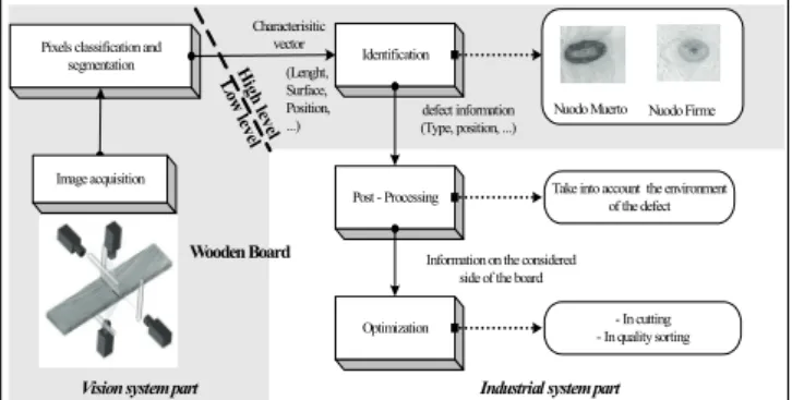
The figure 3 shows an overall description of the industrialist context.

Fig. 3: Wood recognition system.

The classification is performed with the features issued from the segmentation stage which is made by the industrialist. The database is composed of 877 samples divided in nine classes of wood defects (nuodo muerto, grieta, medula, resina …). The industrialist usually works with around 20 features without having any idea about their suitability.

The learning database is composed of 250 samples. The database used to test and validate the feature selection is composed of 627 samples. These databases are relatively heterogeneous, for instance, the 250 samples of the learning database are composed of 8, 56 7, 7, 18, 47, 5, 93, 9 samples of the nine classes. The fuzzy inference engine consists in a single inference where all the features are in input of the model and all the classes to recognize in output.

B. Feature Selection Evaluation

Tests aim to reduce the dimensionality by removing non pertinent parameters until reaching an interpretable model while keeping a “good” recognition rate. Six feature selection methods were used SBFS, SFFS [19], SVM [20] and proposed method FRIF-MS1 and 2.

Classical FRIFS was also applied onto the 10 remaining parameters. At this step recognition rates are 94% for learning and 74.5% for generalization except for SVM where two parameters differ (93.6% and 71%).

Table 1 provides new obtained recognition Tg rates according to removed parameters. Maximal recognition rates are reached with 4-5 parameters ensuring a good interpretability of the model. Until 5 parameters FRIFS-MS1 gives rise to similar results to reference methods (72.25%) and they are close to basic FRIFS method (76.24%) which requires supplementary process.

However as the number of samples per class differs, high recognition rates do no imply a satisfactory recognition for the industrialist. Identification (Lenght, Surface, Position, ...) L ow le_ve l H ig h l_ev el

Pixels classification and segmentation Wooden Board Characterisitic vector defect information (Type, position, ...) Post - Processing Optimization

Information on the considered side of the board

Take into account the environment of the defect - In cutting - In quality sorting Image acquisition Nuodo Firme Nuodo Muerto

TABLE 1. EVOLUTION OF GLOBAL RECOGNITION RATES TG IN

RELATIONSHIP WITH THE NUMBER OF FEATURES.

Table 2 provides obtained results per class with the training data set. The calculated rate Mc represents the means of each class recognition rates Tc. It gives some information about the “good” recognition of each class:

1

1

Mc

Ti

c

=

∑

TABLE 2. COMPARISON OF LEARNING RECOGNTION RATES REACHED PER CLASSES (MC). Method \ Param. Numb. 3 4 5 6 7 8 9 10 FRIFS – MS1 75.4 75.9 79.3 83.2 90.9 95.4 95.4 93.4 FRIFS – MS2 41.8 69.1 74.0 86.6 90.4 95.5 95.4 93.4 FRIFS 66.5 75.9 84.3 91.1 90.9 95.4 95.4 93.4 SBFS/SFFS 33.3 44.4 76.6 86.4 89.8 92.1 92.1 93.4 SVM 71.2 71.2 88.9 88.9 88.8 95.5 94.5 94.5

That shows the good behaviour of our methods following such consideration and that it would be better to keep 6 parameters with FRIFS or 7-8 for others.

C. Classification Comparison

Generalization rates are used to compare the quality of the remaining set of parameters extracted with each method. Such valuation is pointed out by the industrialist: wanted pertinent parameters are those that allow reaching the better recognition rate.

TABLE 3.GENERALIZATION CLASSIFICATION RATES TG OBTAINED USING

THE WHOLE SET OF PARAMETERS (USING FRIFS SELECTED FEATURE SET).

Method \ Param. Numb. 3 4 5 6 7 8 9 10 Bayesian Classifier 41.1 46.0 45.4 46.8 48.1 48.9 49.6 48.9 K-NN 71.7 73.0 75.7 76.7 77.0 79.4 78.1 67.9 Fuzzy K-NN 68.9 72.2 77.0 77.9 78.4 79.1 78.6 69.0 Neural Network 73.3 73.3 75.4 74.8 74.0 77.5 77.1 79.3 Fuzzy Rule Classifier 71.6 75.4 76.2 75.4 75.8 75.3 75.1 71.0 Support Vector Machine 56.8 65.7 64.3 67.2 67.3 68.4 74.5 67.0 The each extracted set obtained using 5 methods (FRIFS, FRIFS-MS1 and 2, SVM [20], SBFS and SFFS [19]) has been provided as an input to several classifiers:

Bayesian (Euclidean distance), K-NN (k=3 or 5), Fuzzy K-NN (K=5), Neural Network (3 hidden layers, 20 neurons/layer), SVM (Gaussian kernel) and FRC (5 Terms) [12] [21].

Table 3 shows the obtained classification rates Tg. It is calculated on the whole database, independently of the classes. They vary from 79.3% using 10 parameters to 73.37% using 3 parameters. A maximum of 80.06% is reached with 6 parameters using NN classifier applied on SFFS parameter set.

However, such recognition rate is not significant because it considers the whole database despite the number of samples is not equal for each class separately. More than the score of 80.06% is only reached by recognizing almost the samples of the classes having the greatest number of samples.

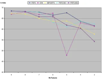
An efficient classifier index Ic is calculated in order to provide a better compromise between the mean (Mc) and the standard deviation (Sc) of class recognition rates Tc and the global recognition rate Tg as follows. Figure 4 shows the variability of Ic.

Ic = Mean ( Mc, Tg, (100 – Sc)) (8) Features /

Methods FRIFS-MS1 FRIFS-MS2 FRIFS SBFS / SFFS SVM

Learn.

Rate 94.0% 94.0% 94.0% 94.0% 93.6% 10

Gener.

Rate 74.5% 74.5% 74.5% 74.5% 71.0% Feat. Sup LR_RE LR_RE LR_RE LR CR3 9

Learn.

Rate 95.2% 95.2% 95.2% 92.0% 93.6% Feat. Sup SURF MJ_AX SURF MJ_AX ORIE 8

Learn.

Rate 95.2% 95.2% 95.2% 92.0% 95.2% Feat. Sup C3 MN_AX C3 DX/DY LR 7

Learn.

Rate 94.4% 94.0% 94.4% 90.4% 87.6%

Feat. Sup C4 C3 MJ_A C3 C3

6

Learn.

Rate 84.0% 93.2% 93.6% 90.0% 88.0% Feat. Sup MJ_A C4 MN_A SURF SURF

Learn.

Rate 82.0% 76.9% 92.4% 84.8% 88.0% 5

Gener.

Rate 72.3% 69.8% 76.2% 71.9% 76.4% Feat. Sup MN_A DX/DY C4 MN_A DX/DY

Learn.

Rate 80.8% 74.8% 80.8% 74.8% 75.6% 4

Gener.

We can notice that remaining features have the same characteristics whatever the underlined method. They refer to the same kind of information even, they are not equal (size, shape, color…).

FRIFS allows achieving in most of the cases the best results which is coherent with others applications based on Fibre [6].

FRIFS-MS1 is the proposed improvement which gives the closer results to the optimal set of features, but FRIFS-MS2 provides very similar results while requiring few learning samples

Fig. 4: Feature selected set comparison with It index.

V. CONCLUDING REMARKS

A “Multi Scale” enhancement of a Fuzzy Rule Iterative Feature Selection method FRIF-MS has been presented in this paper. Performed tests on industrial data confirm the interest of decreasing the number of feature to increase the recognition rate. The results obtained in this wood industrial context are similar with the previously ones obtained in fabric industrial context [6]. Moreover, these results show that the FRIFS method is very efficient in this specific wood context too. Furthermore remaining parameters seems to be more representative of all the classes. The global recognition rate is better than provided by other methods and the recognition is also better for each class. The FRIFS method and its Multi-Scale extensions seem to be efficient in case of both small and heterogeneous data sets.

Actually, the extension of our model to provide features selection per class is under consideration.

REFERENCES

[1] Abdulhady M., Abbas H., Nassar S.: Performance of neural classifiers for fabric faults classification, in proc. IEEE International Joint Conference on Neural Networks (IJCNN '05), Montreal, Canada, (2005) 1995-2000.

[2] Yang X., Pang G., Yung N.: Fabric defect classification using wavelet frames and minimum classification error training, 37th IAS Industry Application Conference, Pittsburgh, PA, USA, vol 1 (2002) 290–296. [3] Murino V., Bicego M., Rossi I.A.: Statistical classification of raw

textile defects in Proc. of the 17th Int. Conf. on Pattern Recognition (ICPR’04), Cambridge, UK, vol 4 (2004) 311- 314.

[4] Kudo, M., Sklansky, J.: Comparison of algorithms that select features for pattern classifiers. Pattern Recognition 33 (2000) 25–41.

[5] Zhang, H., Sun, G.: Feature selection using Tabu Search method. Pattern Recognition 35 (2002) 701–711.

[6] Schmitt E., Bombardier V., Wendling L.: Improving Fuzzy Rule Classifier by Extracting Suitable Features from Capacities with Respect to the Choquet Integral, IEEE Trans. On System, Man and Cybernetics 38 vol 5 (2008) 1195-1206.

[7] Dubois D., Prade H., Fuzzy rules in knowledge-based systems – Modelling gradedness, uncertainty and preference, An introduction to fuzzy logic application in intelligent systems, Kluwer, Dordrecht (1992), 45-68,.

[8] Dubois D., Prade H, What are Fuzzy rules and how to use them?, Fuzzy Sets and Systems, vol. 84 (1996), 169-185.

[9] Mendel J.M., Fuzzy logic systems for engineering: A tutorial, Proceedings of the IEEE vol. 83 (1995), 345–377.

[10] Ishibuchi, H., Nozaki, K., Tanaka, H.: Distributed representation of fuzzy rules and its application to pattern classification. Fuzzy Sets and Systems 52 (1992) 21-32.

[11] Ishibuchi H., Nozaki K.,Tanaka H., A Simple but powerful heuristic method for generating fuzzy rules from numeric data, Fuzzy sets and systems, vol. 86 1997), 251-270.

[12] Bombardier V., Schmitt E., Charpentier P., A fuzzy sensor for color matching vision system, Measurement, Vol 42 (200), 189-201. [13] Grabisch, M., Nicolas, J.M.: Classification by fuzzy integral -

performance and tests. Fuzzy Sets and Systems, Special Issue on Pattern Recognition 65 (1994) 255-271.

[14] M. Grabisch, A new algorithm for identifying fuzzy measures and its application to pattern recognition, Proc. 7th IEEE Int. Joint Conf. Fuzzy Syst., Yokohama, Japan, (1995).

[15] Grabisch, M.: The application of fuzzy integral in multicriteria decision making. Europ. journal of operational research 89 (1995) 445-456.

[16] Shapley, L.: A value for n-person games. Contributions to the Theory of Games, Annals of Mathematics Studies. Khun, H., Tucker, A., (ed.). Princeton University Press (1953) 307-317.

[17] Murofushi, T., Soneda, S.: Techniques for reading fuzzy measures(iii): interaction index. in proc. 9th Fuzzy System Symposium, Sapporo, Japan (1993) 693-696.

[18] Rendek, J., Wendling, L.: Extraction of Consistent Subsets of Descriptors using Choquet Integral. in Proc. 18th Int. Conf. on Pattern Recognition, Hong Kong, Vol. 3 (2006) 208-211.

[19] Pudil P., Novovicova J., Kittler J., Floating search methods in feature selection, Pattern Recognition Letters, vol. 15 (1994), pp. 1119–1125. [20] Grandvalet Y., Canu S., Adaptative Scaling for Feature Selection in

SVMs, Neural Information Processing System (2002).

[21] Michie D., Spiegelhalter D.J.,Taylor, C.C., Machine Learning Neural and Statistical Classification, Ellis Horwood, (1994).

40 45 50 55 60 65 70 9 8 7 6 5 4 3 Nb Features