HAL Id: hal-00996956
https://hal.archives-ouvertes.fr/hal-00996956
Submitted on 27 May 2014HAL is a multi-disciplinary open access archive for the deposit and dissemination of sci-entific research documents, whether they are pub-lished or not. The documents may come from teaching and research institutions in France or abroad, or from public or private research centers.
L’archive ouverte pluridisciplinaire HAL, est destinée au dépôt et à la diffusion de documents scientifiques de niveau recherche, publiés ou non, émanant des établissements d’enseignement et de recherche français ou étrangers, des laboratoires publics ou privés.
HF radar detection of infrasonic waves generated in the
ionosphere by the 28 March 2005 Sumatra earthquake
Alain Bourdillon, Giovanni Occhipinti, Jean-Philippe Molinié, Véronique
Rannou
To cite this version:
Alain Bourdillon, Giovanni Occhipinti, Jean-Philippe Molinié, Véronique Rannou. HF radar de-tection of infrasonic waves generated in the ionosphere by the 28 March 2005 Sumatra earth-quake. Journal of Atmospheric and Solar-Terrestrial Physics, Elsevier, 2014, 109, pp.75-79. �10.1016/j.jastp.2014.01.008�. �hal-00996956�
1
HF radar detection of infrasonic waves generated in the ionosphere by the 28 March 1 2005 Sumatra earthquake 2 3 Alain Bourdillon 4
Institut d’Electronique et Télécommunications de Rennes, Université de Rennes 1,
5
Rennes, France
6
Email : abourdil@free.fr Phone : +33620495756
7 8
Giovanni Occhipinti
9
Institut de Physique du Globe de Paris, Paris, France
10
Email : ninto@ipgp.fr Phone : +33157275307
11
12
Jean-Philippe Molinié
13
Office National d’Etudes et de Recherches Aérospatiales, Palaiseau, France
14
Email : jean-philippe.molinie@onera.fr Phone : +33180386234
15 16
Véronique Rannou
17
Office National d’Etudes et de Recherches Aérospatiales, Palaiseau, France
18
Email : veronique.rannou@onera.fr Phone : +33180386202
2 Abstract
1
Surface waves generated by earthquakes create atmospheric waves detectable in the
2
ionosphere using radio waves techniques: i.e., HF Doppler sounding, GPS and altimeter
3
TEC measurements, as well as radar measurements. We present observations performed
4
with the over-the-horizon (OTH) radar NOSTRADAMUS after the very strong
5
earthquake (M=8.6) that occurred in Sumatra on March 28, 2005. An original method
6
based on the analysis of the RTD (Range-Time-Doppler) image is suggested to identify
7
the multi-chromatic ionospheric signature of the Rayleigh wave. The proposed method
8
presents the advantage to preserve the information on the range variation and time
9
evolution, and provides comprehensive results, as well as easy identification of the waves.
10
In essence, a Burg algorithm of order 1 is proposed to compute the Doppler shift of the
11
radar signal, resulting in sensitivity as good as obtained with higher orders. The
multi-12
chromatic observation of the ionospheric signature of Rayleigh wave allows to extrapolate
13
information coherent with the dispersion curve of Rayleigh waves, that is, we observe two
14
components of the Rayleigh waves with estimated group velocities of 3.8 km/s and 3.6
15
km/s associated to 28 mHz (T~36 s) and 6,1 mHz (T~164 s) waves, respectively. Spectral
16
analysis of the RTD image reveals anyway the presence of several oscillations at
17
frequencies between 3 and 8 mHz clearly associated to the transfer of energy from the
18
solid-Earth to the atmosphere, and nominally described by the normal modes theory for a
19
complete planet with atmosphere. Oscillations at frequencies larger than 8mHz are also
20
observed in the spectrum but with smaller amplitudes. Particular attention is pointed out
21
to normal modes 0S29 and 0S37 which are strongly involved in the coupling process. As
22
the proposed method is frequency free, it could be used not only for detection of
23
ionospheric perturbations induced by earthquakes, but also by other natural phenomena as
3
well as volcanic explosions and particularly tsunamis, for future oceanic monitoring and
1
tsunami warning systems.
2
3
Keywords: HF skywave radar; effects of earthquakes in the ionosphere; Rayleigh wave;
4
atmospheric normal modes
5 6
Highlights 7
We observe large scale oscillations of the ionosphere induced by an earthquake.
8
We suggest a method to identify the multi-chromatic components of the
9
oscillations.
10
We identify the main atmospheric normal modes at frequencies between 3 and 8
11
mHz.
12
Weaker atmospheric modes are observed at higher frequencies, at least up to 30
13
mHz.
14 15
4 1. Introduction
1
Dynamic coupling between the solid and fluid part of the Earth system clearly shows that
2
the vertical displacement of the ground and the ocean following seismic events creates
3
acoustic-gravity waves propagating in the neutral-atmosphere, which are detectable in the
4
ionosphere using radio waves techniques (Peltier & Hines, 1976; Lognonné et al., 1998;
5
Occhipinti et al. 2008). Several mechanisms are able to excite atmospheric
acoustic-6
gravity waves, for instance explosions at/or under the surface of the Earth (Broche, 1977;
7
Blanc, 1985; Calais et al., 1998), volcanic eruptions (Kanamori and Mori, 1992; Hao et
8
al., 2006), tsunamis (Occhipinti et al., 2006, 2008, 2011; Rolland et al., 2010), and
9
earthquakes at both the source region (Rolland et al., 2011, Astafyeva et al., 2011) or at
10
the teleseismic distances induced by Rayleigh waves propagation (Najita and Yuen, 1979;
11
Tanaka et al., 1984; Ducic et al., 2003; Artru et al., 2005; Hao et al., 2006; Occhipinti et
12
al., 2010). Though the Rayleigh wave is the main contributor to the acoustic-wave
13
excitation, it has been reported by Chum et al. (2012) that the seismic P and S waves
14
could also play a role. For a clear review of the post-seismic ionospheric perturbations,
15
highlighting the difference between observations in the far-field and observations close to
16
the epicenter, we refer to Occhipinti et al. (2013).
17
The seismic Rayleigh wave created by an earthquake propagates at the ground-surface
18
covering several times the Earth’s circumference (figure 1). The vertical displacement
19
induced by Rayleigh waves at the teleseismic distance induces, by dynamic coupling, an
20
acoustic wave propagating vertically in the atmosphere. During the upward propagation,
21
this acoustic wave is strongly amplified by the double effect of the conservation of energy
22
and the exponential decrease of the atmospheric density with altitude. At ionospheric
23
altitudes this growing acoustic wave induces strong perturbation in the plasma density and
5
plasma velocity which could be detected by Doppler soundings, Total Electron Content
1
(TEC) measurements by GPS or altimeters, and HF skywave radars.
2
Doppler sounding is a very sensitive method and it has been extensively used to study the
3
ionospheric signature of Rayleigh waves (Najita and Yuen, 1979; Artru et al., 2005;
4
Occhipinti et al., 2010). The Global Positioning System (GPS) allows the estimation of
5
Total Electron Content (TEC) fluctuations, that is, the variation of the plasma density
6
integrated between a ground receiver and the GPS satellite (Mannucci et al., 1998).
7
Additionally, the dense GPS network allows the imaging with high resolution maps of
8
TEC perturbations showing the signature of Rayleigh waves over large areas (Ducic et al.,
9
2003; Rolland et al., 2011). The capability of an over-the-horizon (OTH) radar to detect a
10
Rayleigh wave signature in plasma velocity has been already proved by Occhipinti et al.
11
(2010) during the Sumatra earthquake (M=8.6) on 28 March 2005 at 16:09:36 UT,
12
therefore validating the signature on the OTH radar by comparison with modeling and
13
Doppler sounder data.
14
In this work we present an additional and self-sufficient method to analyze the
15
Nostradamus HF radar data collected on the 28 March 2005 event, which is based on
16
Range-Time-Doppler (RTD) imaging. The presented methodology shows a richer spectral
17
signature of the detected wave and allows a direct estimation of the wave speeds. In
18
addition, large scale oscillations of the ionosphere are reported for first time, which
19
correspond to the atmospheric normal-modes excited by the Rayleigh waves mainly in the
20 frequency range 3-8 mHz. 21 22 2. Radar data 23
6
Nostradamus is a mono-static OTH radar located in Normandy, west of Paris. Following
1
the characteristic of OTH radar, the electromagnetic HF signal emitted by the radar is
2
reflected by the ionosphere, and then backscattered by the ground and, following the same
3
path, it travels back to the radar. The emission/reception antenna-array comprises 288
4
antennas organized in three arms oriented at 120° and allowing emission beam forming
5
capability with 10°-80° elevation and 360° azimuth freedom (Bazin et al., 2006). If the
6
time interval between two different measurements is long enough, a double reflection (2F)
7
is also detectable. On 28 March 2005, the radar was not operational at the onset of the
8
earthquake. Consequently, the measurements started only after the reception of a seismic
9
alert, but not early enough to catch the signature of the first Rayleigh wave (R1) reaching
10
the Nostradamus sounding area (Figure 1). Rayleigh waves generated after the rupture
11
propagate several time around the Earth surface; the radar emission beam was oriented in
12
azimuth 270° W and elevation 30° in order to catch the arrival of the Rayleigh wave (R2)
13
reaching the Nostradamus sounding area by the longest path (Occhipinti et al., 2010). For
14
the R2 path the spherical distance on the Earth surface between the earthquake epicenter
15
and the radar is about 29750 km. The frequency of the wave transmitted by the radar was
16
set at 7.85 MHz with a pulse repetition frequency (PRF) fixed at 50 Hz.
17
The energy backscattered at the ground and received by the Nostradamus radar in March
18
28, 2005 between 18:11:43 to 18:48:28 UT, is shown in the Range-Time-Intensity (RTI)
19
image of Figure 2. We observe two main energetic responses consisting of a double
20
reflection: a one hop propagation mode (1F), observed with group paths between
820-21
1000 km, followed by a second hop (2F) that correspond to group paths larger than 1600
22
km (Figures 1 and 2). Weak echoes are also observed between the two main echoes.
23
To analyze the propagation modes of the radio wave, a quasi-parabolic layer was
24
introduced into the ray-tracing program developed by Mlynarczyk et al. (2000). The
7
ionospheric parameters were obtained from the Fairford ionosonde (UK): critical
1
frequency foF2=6 MHz, height of maximum plasma density hm=250 km. At that time of
2
the day during March at midlatitudes, the E layer can be neglected so that a single F2
3
layer may represent the ionosphere with sufficient accuracy for oblique ray-tracing. The
4
half-thickness was fixed at ym=100 km. The results of ray-tracing are summarized in table
5
1. In essence, for a 30° elevation angle the radio wave reflection occurs at 179 km height,
6
the group path is GP=811 km and the ground range is GR=680 km. For smaller elevation
7
angles the range increases which is the reason for the observed range-spread of radar
8
echoes (up to 1000 km in figure 1 for a one hop mode). Neglecting horizontal density
9
gradients in the ionosphere, the group path and ground ranges for a double hop are twice
10
the values obtained for a single hop mode: GP=1622 km and GR=1360 km at 30°
11
elevation angle. Consequently, the difference in ground range of the sub-ionospheric
12
reflection points for 2F and 1F at 30° elevation angle is GR(2F)-GR(1F)=680 km. Table 1
13
shows that for elevation angles varying between 20° and 35° the reflection height varies
14
between 164 km and 189 km.
15
Although figure 2 does not display a clear signature of a wave pattern in the RTI image,
16
we show in the next paragraph that wave patterns do exist in the RTD image. This is
17
because, in this case, the power of the radar echoes is largely insensitive to ionospheric
18
waves contrary to the Doppler shift which is rather sensitive.
19
20
3. The ionospheric waves 21
In order to highlight the presence of the atmospheric Rayleigh wave signature in the
22
Nostradamus data, we analyze the RTD plot produced using the Burg algorithm with an
23
order 1 (Figure 3). The Burg algorithm estimates the spectral content by fitting an
8
regressive (AR) process of a given order. Here we used the algorithm provided in the
1
MATLAB signal processing toolbox. In every range resolution cell the Doppler shift at
2
the maximum of spectral power is plotted using a color scale spanning between +0.3 and
-3
0.5 Hz. An oscillation in the Doppler shift is observed in the first half of the image,
4
forming patterns with tilted striations on the 2F mode (A) and also on the 1F mode (B).
5
The Doppler shift oscillates approximately with 0.2 Hz peak to peak amplitude and a 28
6
mHz frequency. The oscillation appears first on the 2F mode and later in the 1F mode
7
after being delayed by approximately 180 s. For a 680 km range difference between the
8
two reflection points (2F-1F), the group velocity estimate is Vg~ 3.8 km/s, which is in
9
accordance with the speed of Rayleigh waves.
10
The presence of two reflection points (1F and 2F) could easily explain the two waves
11
observed by Occhipinti et al. (2010). We highlight that Occhipinti et al. (2010) only
12
explain the wave observed at around 18:40 UT by comparing it with modeling and
13
Doppler sounder data.
14
As the Rayleigh waves R2 move from the West to the East (Figure 1), they are observed
15
earlier on the 2F mode at 18:20 UT. For the 28 mHz wave the propagation time for the R2
16
path is 7824 s. A smaller frequency wave with f~ 6.1 mHz appears at 18:32 UT on the 2F
17
mode (C) with a 8484 s propagation time and at 18:35 UT on the 1F mode (D). The
18
propagation time of the waves includes 2 contributions: the propagation time of the
19
Rayleigh wave excited at the earthquake epicenter plus the propagation time of the
20
infrasonic wave from the ground up to the observation point (~180 km altitude). The
21
propagation time of the infrasonic waves, estimated from the results published by Najita
22
and Yuen (1979) were assumed to be 6 min for the 28 mHz wave and 10 min for the 6.1
23
mHz wave. With a 28730 km distance between the epicenter and the subionospheric point
24
of the 2F mode, the group velocity estimates of the Rayleigh waves are 3.8 km/s and 3.6
9
km/s for these two waves, respectively. These estimates are in agreement with the
1
Rayleigh wave dispersion curve and previous observations by ionospheric sounding
2
(Najita & Yuen, 1979; Ducic et al., 2003).
3
The vertical air particle motion Un producing the Doppler shift fD is given by: 4
5
where f is the radar frequency, c the speed of light, I the Earth magnetic field inclination
6
and E the elevation angle of the radar beam. For f=7.85 MHz, I=63° and E=30°, a 0.2 Hz
7
Doppler shift corresponds to a 4.8 m/s vertical velocity. The ratio of the air particle
8
velocity at ground level to the air particle velocity in the atmosphere depends
9
mainly on wave frequency, altitude and atmospheric conditions. If we assume a ratio
10
in the range 2-4 104 at 180 km altitude (Artru et al., 2001), the vertical velocity of 11
the ground during the event is estimated to be between about 0.12 to 0.24 mm/s. Here we
12
assumed only advective motions of the layer but we neglected the contribution of the
13
compression term which could play a role for the low period infrasound waves (Chum et
14
al., 2012). We additionally highlight that the amplitude of the oscillation observed by
15
OTH radar was already reproduced numerically by normal mode summation by
16
Occhipinti et al. (2010), validating the accord with the seismic displacement in the
17
observation zone as well as the sources parameters of the event.
18 19
4. Solid Earth-Atmosphere coupling 20
10
A more accurate spectral analysis of the Doppler time series by FFT processing confirms
1
that several components are clearly visible close to the main signature at 6.1 mHz.
2
The coupling theory between solid Earth and atmosphere under normal mode formulation
3
(Lognonné et al., 1998, Artru et al., 2001), which is supported by different observations
4
(Kanamori and Mori, 1992; Nishida et al., 2000; Occhipinti et al., 2010), clearly shows
5
that the energy of surface Rayleigh waves is mainly transferred into the
6
atmosphere/ionosphere following the preferential modes 0S29 and 0S37 at 3.7 and 4.4
7
mHz, respectively.
8
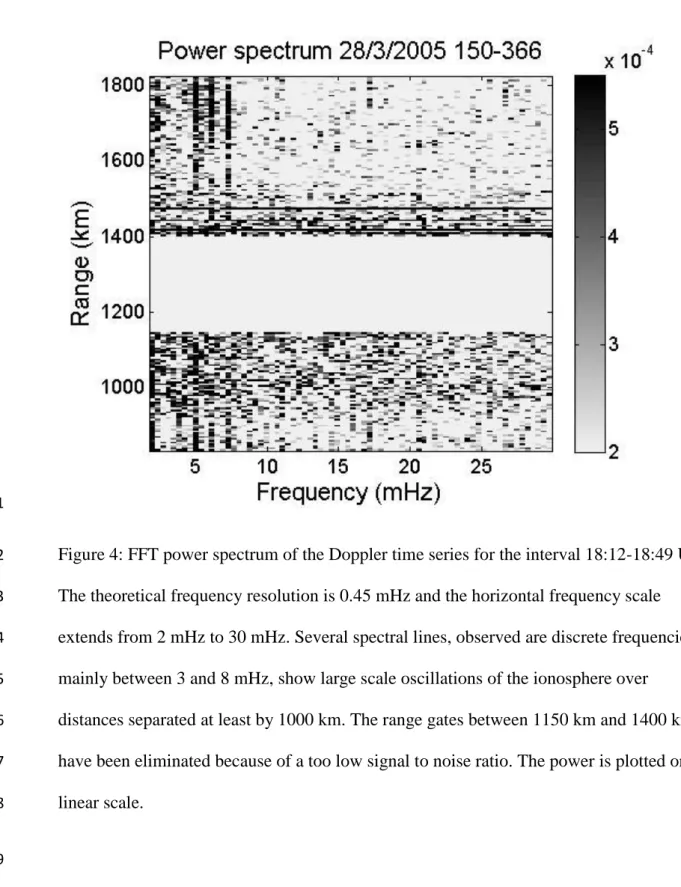
By performing FFT analysis of the time series obtained with the Doppler values at a given
9
radar range, and repeating the computation for every line of RTD, we obtained the
10
spectrum presented in figure 4. Since the time series have 2205 seconds duration, the
11
theoretical frequency resolution is 0.45 mHz. As seen, several spectral lines are observed
12
between 3 and 8 mHz at frequencies which are independent of range. This simply
13
highlights the fact that the radar observes large scale oscillations coherent over, at least,
14
1000 km: in essence the signature of the Rayleigh wave propagating on the Earth surface
15
and its signature in the ionosphere. Note that for ranges between 1150 and 1540 km the
16
values are set to zero because of the too low signal to noise ratio.
17
The power spectrum averaged for ranges between 823 km and 1823 km is presented in
18
figure 5. As described by the coupling theory a large amount of the energy is observed
19
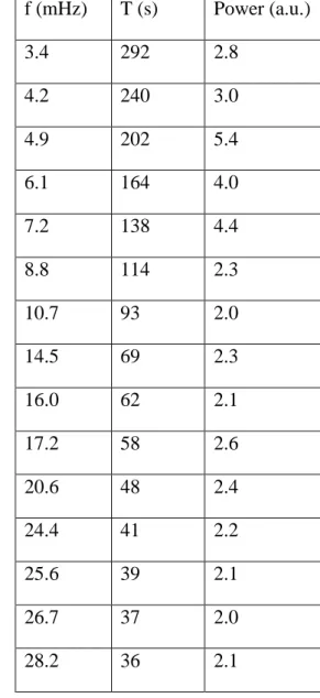
between 3 and 8 mHz. Table 2 lists the frequency, the period and the power of the main
20
peaks in the band 2-30 mHz. This table highlights the presence of oscillations at
21
frequencies close to the theoretical values 3.7 mHz and 4.4 mHz, corresponding
22
respectively to the normal modes 0S29 and 0S37 and directly linked to the atmospheric
23
signature of Rayleigh waves. The five strongest peaks are observed at 3.4 mHz, 4.2 mHz,
11
4.9 mHz, 6.1 mHz and 7.2 mHz thus the smallest frequency oscillations found in the radar
1
observations are close to the values obtained by normal mode modeling (i.e., Artru et al.,
2
2001). Large-scale oscillations also exist at frequencies above 8 mHz but with weaker
3 amplitudes. 4 5 5. Discussion - conclusion 6
Doppler analysis of HF radar signal provides information on waves propagating in the
7
ionosphere over large areas. Based on the RTD and spectral analysis we highlight the
8
presence of waves propagating in the ionosphere that represent the plasma signature of
9
Rayleigh waves generated by the seismic event in Sumatra (M: 8.6; 28 March, 2005). Two
10
main waves are observed: (1) one wave with a frequency 28 mHz frequency (T~36 s) and
11
a group velocity of Vg= 3.8 km/s, (2) and a second wave with a 6.1 mHz frequency
12
(T~160 s), moving with a group velocity of Vg= 3.6 km/s. These values are consistent
13
with the dispersion curve of Rayleigh waves. The delay between the time of arrival of the
14
two waves is of the order of 11 min; this delay contains the difference in the propagation
15
time of the two infrasonic waves in the atmosphere (~4 min), as well as the difference (~7
16
min) in the propagation time of the Rayleigh wave propagating on the Earth surface due to
17
the dispersion of Rayleigh waves and the consequent variation of the group velocities at
18
frequencies 28 mHz (36 s) and 6.1 mHz (160 s), respectively.
19
Occhipinti et al. (2010) have already studied the NOSTRADAMUS data of the 28 March
20
2005 event. They highlight the presence of the signature of a Rayleigh wave in the
21
ionosphere by comparison with modeling and Doppler sounding measurements, but they
22
consider only one range gate, consequently the signal arriving at around 18.20 UT
23
remained unexplained. Moreover, the radar signal was filtered in the 3-7 mHz band,
12
eliminating the 28 mHz (36 s) wave and leaving only the long period wave. Our work
1
clearly highlights the presence of a double hop and a consequent double range gate,
2
clearly showing that the ionospheric signature of Rayleigh waves is observed twice by the
3
OTH radar. As a result, it was possible to measure the local speed of Rayleigh wave by
4
comparison between the two observed echoes linked to the two hops.
5
Additionally, a more detailed spectral analysis clearly showed a multi-chromatic signal on
6
both range gates, showing that the same waves are observed on both hops. Most of the
7
common excited frequencies with high energy were observed between 3 mHz and 8 mHz
8
in agreement with the theory of the solid-Earth/atmosphere coupling. With particular
9
attention, two signals were observed at 3.4 mHz and 4.2 mHz, that is, at frequencies close
10
to the 0S29 and 0S37 modes, which are mainly involved in the Rayleigh wave transfer of
11
energy from the solid Earth to the atmosphere.
12
In the ionosphere, there exist different sources of short period Doppler fluctuations which
13
may not relate with infrasonic waves, for instance the geomagnetic pulsations (Sutcliffe
14
and Poole, 1984, Bourdillon et al., 1989, Liu and Berkey, 1993, Anderson and
15
Abramovich, 1998). Therefore, it is important for such studies to identify that the source
16
of the waves observed by the radar are in association with infrasonic waves generated by
17
earthquakes and therefore exclude magneto hydrodynamic effects or other sources of
18
perturbations. This is not an easy task which requires other sources of data.
19
A Burg algorithm with an order 1 was applied here with a 10.24 s integration time to
20
generate RTD images. Higher orders (up to 7) have been tried but without a significant
21
improvement in both the RTD images and FFT processing. Since this method can reveal
22
effectively wave propagation effects on RTD images regardless of any frequency range
23
limits, we conclude that it can potentially be extended also in tsunami detection.
13
Obviously, the detection of tsunami waves is still of major concern for countries close to
1
active seismic regions. Tsunamis, which are usually generated by submarine earthquakes,
2
are supposed to produce internal gravity waves, with periods 8-40 min, propagating
3
obliquely upward in the atmosphere and consequently perturbing the ionosphere. Though
4
the wave amplitude at sea surface is small (few centimeters) the atmosphere provides an
5
amplification mechanism by a factor of about 104 when the wave reaches the lower F
6
layer.
7
The detection of tsunamis by ionospheric monitoring was theoretically proposed initially
8
by Peltier and Hines (1976) and extensively validated by Occhipinti et al. (2006, 2008,
9
2011) by the comparison between observations and numerical mode predictions for the
10
tremendous Sumatra 2004 and Tohoku 2011 events. The generalization to moderate
11
events has been recently proposed by Rolland et al. (2010). Most of the tsunami
12
observations by remote techniques have been performed by Altimeters and GPS observing
13
the TEC variations, and more recently by measurements of airglow (Makela et al., 2011,
14
Occhipinti et al., 2011).
15
The potential detection of tsunamis by OTH radar and by ionospheric monitoring has been
16
explored theoretically by Coïsson et al. (2011) and a more direct observation of tsunamis
17
by HF skywave radar has been addressed by Anderson (2011) in a chapter book. In
18
particular, Anderson (2011) discussed the possibility that tsunami-generated infrasonic
19
emissions and tsunami-generated magneto hydrodynamic perturbations could have a
20
signature on HF skywave signals, which, if identified, could be exploited in tsunami
21
warning systems. In this context, spectral analysis of RTD images could be evolved as a
22
powerful tool to help identify the ionospheric waves associated with earthquakes and
23
tsunamis.
14 1
Acknowledgments 2
Funding for this study was provided by the ONERA – MASCOTH/2012 research
3
program. G.O. is also supported by the CNES and the PNTS/INSU program. We thank P.
4
Dorey for useful discussions about the processing of radar data. This is IPGP contribution
5 3476. 6 7 References 8
Anderson, S., 2011. HF skywave radar performance in the tsunami detection and
9
measurement role, in: The tsunami threat - research and technology, ISBN:
978-953-307-10
552-5.
11
Anderson, S., Abramovich, Y.I., 1998. A unified approach to detection, classification and
12
correction of ionospheric distortion in HF skywave radar systems. Radio Sci., 33, 1055–
13
1067.
14
Artru, J., Lognonné, P., Blanc, E., 2001. Normal modes modelling of post-seismic
15
ionospheric oscillations. Geophys. Res. Lett., 28, 697-700.
16
Artru, J., Ducic, V., Kanamori, H., Lognonné, P., Murakami, M., 2005. Ionospheric
17
detection of gravity waves induced by tsunamis. Geophys. J. Int., 160, 840-848.
18
Astafyeva, E.I., Lognonné, P., Rolland, L., First ionospheric images of the seismic fault
19
slip on the example of the Tohoku-oki earthquake. Geophys. Res. Lett., 38, 2011, L22104,
20
DOI: 10.1029/2011GL049623.
15
Bazin, V., Molinié, J.P., Munoz, J., Dorey, P., Saillant, S., Auffray, G., Rannou, V.,
1
Lesturgie, M., 2006. Nostradamus: An OTH Radar. Aerosp. and Elec. Sys. Mag., IEEE,
2
21, 3-11.
3
Bourdillon, A., Delloue, J., Parent, J., 1989. Effects of geomagnetic pulsations on the
4
Doppler shift of HF backscatter radar echoes. Radio Sci., 24, 183-195.
5
Blanc, E., 1985. Observations in the upper atmosphere of infrasonic waves from natural or
6
artificial sources: A summary. Ann. Geophys., 3, 673-688.
7
Broche, P., 1977. Propagation des ondes acoustico gravitationnelles excitées par des
8
explosions. Ann. Geophys., 33, 281-288.
9
Calais, E., Minster, J.B., Hofton, M.A., Hedlin, M.A.H., 1998. Ionospheric signature of
10
surface mine blasts from Global Positioning System measurement. Geophys. J. Int., 132,
11
191-202.
12
Chum, J., Hruska, F., Zednik, J., Lastovicka, J., 2012. Ionospheric disturbances
13
(infrasound waves) over the Czech Republic excited by the 2011 Tohoku earthquake. J.
14
Geophys. Res., 117, A08319, doi: 10.1029/2012JA017767.
15
Coïsson, P., Occhipinti, G., Lognonné, P., Molinié, J.P., Rolland, L.M., 2011. Tsunami
16
signature in the ionosphere: A simulation of OTH radar observations. Radio Sci., 46,
17
RS0D20, doi:10.1029/2010RS004603.
18
Ducic, V., Artru, J., Lognonné, P., 2003. Ionospheric remote sensing of the Denali
19
earthquake Rayleigh surface waves. Geophys. Res. Lett., 30, 1951-1954.
20
Hao, Y.Q., Xiao, Z., Zhang, D.H., 2006. Response of the ionosphere to the great Sumatra
21
earthquake and volcanic eruption of Pinatubo. Chin. Phys. Lett., 23, 1955-1957.
16
Kanamori, H., Mori, J., 1992. Harmonic excitation of mantle Rayleigh waves by the 1991
1
eruption of Mount Pinatubo, Philippines. Geophys. Res. Lett. ,19, 721-724.
2
Liu, J. Y., Berkey, F.T., 1993. Oscillations in ionospheric virtual height, echo amplitude
3
and Doppler velocity: theory and observations. J. Geomag. Geoelectr., 45, 207-217.
4
Lognonné, P., Clévédé, E., Kanamori, H., 1998. Computation of seismograms and
5
atmospheric oscillations by normal-mode summation for a spherical Earth model with
6
realistic atmosphere. Geophys. J. Int., 135, 388-406.
7
Makela, J. J., Lognonné, P., Hébert, H., Gehrels, T., Rolland, L., Allgeyer, S., Kherani, A.,
8
Occhipinti, G., Astafyeva, E., Coïsson, P., Loevenbruck, A., Clévédé, E., Kelley, M. C.,
9
Lamouroux, J., 2011. Imaging and modelling the ionospheric response to the 11 March
10
2011 Sendai Tsunami over Hawaii. Geophys. Res. Lett., 38, L00G02,
11
doi:10.1029/2011GL047860.
12
Mannucci, A.J., Wilson, B.D., Yuan, D.N., Ho, C.H., Lindqwister, U.J., Runge, T.F.,
13
1998. A global mapping technique for GPS-derived ionospheric electron content
14
measurements. Radio Sci. 33, 565–582.
15
Mlynarczyk, J., Caratori, J., Nowak, S., 2000. Analytical calculation of the radio wave
16
trajectory in the ionosphere. XXIV International Conference IMAPS – Poland, Rytro 25–
17
29 September 2000, p. 347–353.
18
Najita, K., Yuen, P.C., 1979. Long-period Rayleigh wave group velocity dispersion curve
19
from HF Doppler sounding of the ionosphere. J. Geophys. Res., 84, 1253-1260.
20
Nishida, K., Kobayashi, N., Fukao, Y., 2000. Resonant oscillations between the solid
21
Earth and the atmosphere. Science, 287, 2244-2246.
17
Occhipinti, G., Lognonné, P., Alam Kherani, E., Hébert, H., 2006. Three-dimensional
1
waveform modeling of ionospheric signature induced by the 2004 Sumatra tsunami.
2
Geophys. Res. Lett., 33, L20104, doi:10.1029/2006GL026865.
3
Occhipinti, G., Alam Kherani, E., Lognonné, P., 2008. Geomagnetic dependence of
4
ionospheric disturbances induced by tsunamigenic internal gravity waves. Geophys. J. Int.,
5
doi:10.1111/j.1365- 246X.2008.03760.x.
6
Occhipinti, G., Dorey, P., Farges, T., Lognonné, P., 2010. Nostradamus: The radar that
7
wanted to be a seismometer. Geophys. Res. Lett., 37, L18104,
8
doi:10.1029/2010GL044009.
9
Occhipinti, G., Coïsson, P., Makela, J.J., Allgeyer, S., Kherani, A., Hébert, H., Lognonné,
10
P., 2011. Three dimensional numerical modeling of tsunami related internal gravity waves
11
in the Hawaiian atmosphere. Earth Planets Space, 63, doi:10.5047/eps.2011.06.051.
12
Occhipinti, G., Rolland L, Lognonné P, Watada S., 2013. From Sumatra 2004 to
Tohoku-13
Oki 2011: The systematic GPS detection of the ionospheric signature induced by
14
tsunamigenic earthquakes, J. Geophys. Res. Space Physics, 118, doi:10.1002/jgra. 50322.
15
Peltier, W.R., Hines, C.O., 1976. On the possible detection of tsunamis by a monitoring of
16
the ionosphere. J. Geophys. Res., 81, 1995-2000.
17
Rolland, L., Occhipinti, G., Lognonné, P., Loevenbruck, A., 2010. The 29 September
18
2009 Samoan tsunami in the ionosphere detected offshore Hawaii. Geophys. Res. Lett.,
19
37, L17191, doi:10.1029/2010GL044479.
20
Rolland, L.M., Lognonné, P., Munekane, H., 2011. Detection and modeling of Rayleigh
21
wave induced patterns in the ionosphere. J. Geophys. Res., 116, A05320,
22
doi:10.1029/2010JA016060.
18
Sutcliffe, P.R., Poole, A.W.V., 1984. Low latitude Pc3 pulsations and associated
1
ionospheric oscillations measured by a digital chirp ionosonde. Geophys. Res. Lett., 11,
2
1172-1175. doi:10.1029/GL011i012p01172.
3
Tanaka, T., Ichinose, T., Okuzawa, T., Shibata, T., Sato, Y., Nagasawa, C., Ogawa, T.,
4
1984. HF-Doppler observations of acoustic waves excited by the Urakawa-Oki earthquake
5
on 21 March 1982. J. Atmos. Terrest. Phys., 46, 233-245.
19
Table 1: Range, group path and height of reflection versus site angle.
1
Site angle (°) Range (km) Group Path (km) Height (km)
20 25 30 35 882 760 680 629 964 863 811 795 164 171 179 189 2 3
Table 2: Spectral components measured on the averaged spectrum: frequency (mHz), period
4
(s), power (arbitrary unit).
5 f (mHz) T (s) Power (a.u.) 3.4 292 2.8 4.2 240 3.0 4.9 202 5.4 6.1 164 4.0 7.2 138 4.4 8.8 114 2.3 10.7 93 2.0 14.5 69 2.3 16.0 62 2.1 17.2 58 2.6 20.6 48 2.4 24.4 41 2.2 25.6 39 2.1 26.7 37 2.0 28.2 36 2.1 6
20 1
2
3
Figure 1: schematic vision of the propagation of the Rayleigh waves and its signature in
4
the atmosphere, respectively, around the planet (small figure, from Occhipinti et al. 2010),
5
and on the European continent for the phase R2 in the zone sounded by Nostradamus at
6
the two reflection points 1F and 2F (main figure). The blue and red curves show a
7
schematic of a wave front on the ground (R2) and in the atmosphere (R2 atmo) with
8
eastward propagation (red arrow). R indicates the radar location.
9
10 11
21 1
2
Figure 2: RTI plot recorded on 28 March 2005 in azimuth 270° and site 30°. The vertical
3
axis represents the group path (GP) with a 5 km resolution and the horizontal axis
4
represents the universal time with a 10.24 s resolution. A one hop propagation mode (1F)
5
is first observed with group paths between 820-1000 km and a second hop (2F) is obtained
6
for group paths greater than 1600 km. Weak echoes are also observed between the two
7
main echoes. The color scale represents the received power in dB.
8 9
22 1
2
Figure 3: RTD image recorded on 28 March 2005 in azimuth 270° and site 30°. The
3
vertical axis represents the group path (GP) with a 5 km resolution and the horizontal axis
4
is universal time with a 10.24 s resolution. The color represents the Doppler shift
5
computed using the Burg algorithm with an order 1. A negative Doppler shift oscillating
6
with a 36 s period is observed to start at 18:20 UT on the 2F mode (A) and at about 18:23
7
UT on the 1F mode (B). An oscillation in the Doppler shift is observed in the first half of
8
the image, forming patterns with tilted striations on the 2F mode (A) and also on the 1F
9
mode (B). Due to the weak signal to noise ratio the time of arrival is not precisely
10
determined. A lower frequency wave with f~ 6.1 mHz appears at 18:32 UT on the 2F
11
mode (C) and at 18:35 UT on the 1F mode (D).
12
13 14
23
1
Figure 4: FFT power spectrum of the Doppler time series for the interval 18:12-18:49 UT.
2
The theoretical frequency resolution is 0.45 mHz and the horizontal frequency scale
3
extends from 2 mHz to 30 mHz. Several spectral lines, observed are discrete frequencies,
4
mainly between 3 and 8 mHz, show large scale oscillations of the ionosphere over
5
distances separated at least by 1000 km. The range gates between 1150 km and 1400 km
6
have been eliminated because of a too low signal to noise ratio. The power is plotted on a
7
linear scale.
8 9
24 1
Figure 5. Spectrum of the Doppler time series averaged for ranges between 834 km and 1823
2
km, for the time interval 18:12-18:48 UT. The intermediate zone, for ranges between 1150 km
3
and 1400 km, where the S/N ratio is too low, has been excluded from the average. The
4
horizontal frequency scale extends from 2 to 30 mHz. The strongest peaks are observed
5
between 3 mHz and 8 mHz. Weaker peaks are observed at larger frequencies, up to 30 mHz.
6 7