MINISTÈRE DE L’ENSEIGNEMENT SUPÉRIEUR ET DE LA RECHERCHE SCIENTIFIQUE
Université des Sciences et de la Technologie d’Oran Mohammed Boudiaf
USTO-MB
FACULTÉ DE GÉNIE MÉCANIQUE DÉPARTEMENT DE GÉNIE MÉCANIQUE
THÈSE
En vue de l’obtention du diplôme de doctorat en sciences en génie mécanique
SPÉCIALITÉ: GÉNIE MÉCANIQUEOPTION: GÉNIE MÉCANIQUE Présentée par:
Mr. Lakhdar AIDAOUI
INTITULÉE
Soutenu publiquement le: 24.06.2015 devant le jury composé de:
Mme. Amina SABEUR Pr USTO-MB Oran Présidente
Mr. Abbès AZZI Pr USTO-MB Oran Rapporteur
Mr. Alberto MAURIZI Dr ISAC-CNR Bologne (Italie) Co-Rapporteur
Mr. Nouredine SAD CHEMLOUL Pr UIK Tiaret Examinateur
Mr. Ahmed Zineddine DELLIL Pr U Oran Examinateur
Mme. Fadela NEMDILI Dr USTO-MB Oran Examinatrice
MODÉLISATION DE LA POLLUTION PHOTOCHIMIQUE
DE L'AIR À L'ÉCHELLE LOCALE ET MÉSO
Evaluation of the spatial and temporal distribution of nitrogen dioxide (NO2) and Ozone (O3) concentration at local-scale and meso-scale has attracted much interest from the scientific community, from both monitoring and modelling points of view. Photochemical air pollution modelling and simulation in different atmospheric scales was performed during this study.
In the first part of this work, the photochemical smog formation over a heavily industrialized area with complex terrain was investigated. A prognostic meteorological and air pollution model was used in combination with data, which were collected by in situ and remote monitoring stations. The results showed a considerable skill of the model in predicting the major local scale features affecting the pollutants’ dispersion and concentrations in the area of interest. Numerical simulation data of photochemical pollutants were significantly correlated with meteorology during the simulation period. The correlation reveals the most important factors of ozone production, such as solar radiation, temperature, wind speed and topography.
In the second part of the study, NO2 tropospheric vertical column density (VCD) was simulated at different resolutions using the online-coupled BOLCHEM model, with focus to high-polluted regions. High and low-resolution model output are compared to ozone monitoring instrument (OMI) data from the Tropospheric Emission Monitoring Internet Service (TEMIS) over selected areas for the year 2007. For this purpose, satellite data were averaged and regridded on daily basis, onto a common analysis grid with the same model resolutions. Moreover, model simulation results were processed using the averaging kernel (AK) information. The same criteria used to select satellite data, were used as a mask that is applied to model results to make the satellite and model datasets fully consistent. Standard statistical analysis reveals good model performances, even in highly polluted regions, with spatial correlation that ranges from 0.74 to 0.91, depending on the region and model resolution considered. Seasonal analysis shows some dependency on time, with lowest scores in winter, when the satellite product also suffers weaker statistical significance due to the presence of clouds. The increase in resolution is found to affect the spatial correlation of the two high-polluted regions differently, 5% and 23%. This difference is likely to depend on the very different meteorology of the two hot-spots.
Keywords: Photochemical simulation, Tropospheric NO2 column, Model resolution effect,
زوحي مييقت عزوتلا يعضوملا و ينمزلا راشتنﻻ زيكارت يئانث ديسكأ نيجورتينلا NO2 اذكو نوزوألا O3 ىلع نييوتسملا يلحملا و ,طسوتملا ىلع مامتها ناجل ثحبلا ةيملعلا ءاوس نم ةيحان ةبقارملا ىلإ قرطتلا مت ةساردلا هذه لالخ .ةجذمنلا وأ .يوجلا فالغلا يف تايوتسم ةدع ىلع ءاوهلل يئايميكوتوفلا ثولتلا ةاكاحم و ةجذمن .ةدقعم سيراضت تاذ ةيعانص ةقطنم ىوتسم ىلع ةيئايميكوتوفلا مويغلا لكشت ةسارد مت ,عورشملا اذه نم لوألا ءزجلا يف ةرفوتملا تاطحملا نم ةذوخأملا سايقلا تانايب بناج ىلا ,ةيوجلا داصرألا و ءاوهلا ثولتب صاخ جذومن مادختسا مت ثيح مهأب ؤبنتلا يف جمانربلل ةيلاع ةقد لمعتسملا جذومنلا فرط نم اهيلع لصحتملا جئاتنلا ترهظأ .ةقطنملا سفن ىوتسم ىلع نيب ةقالعلا تحضو ةزجنملا ةيمقرلا ةاكاحملاو .مامتهإلا تاذ ةقطنملا ىوتسم ىلع اهزيكارتو تاثولملا عزوت يف ةرثؤملا لماوعلا يف ةرثؤملا لماوعلا مهأ ةقالعلا هذه ترهظأ ثيح ,ةاكاحملا ةرتف لالخ ةيوجلا داصرألا رصانع و يئايميكوتوفلا ثولتلا نوزوألا نوكت O3 .ةقطنملل ةبعصلا سيراضتلا ىلإ ةفاضإلاب حايرلا ةعرس ,ةرارحلا ةجرد ,يسمشلا عاعشإلا لثم , ةيناكم سيياقم ةدع لامعتساب نيجورتينلا ديسكأ يناثل ةيدومعلا ةفاثكلا ةاكاحم تمت ,ةساردلا هذه نم يناثلا ءزجلا لالخ جمانربلا مادختساب كلذ و ةقدلل BOLCHEM ةيداعلا و ةيلاعلا ةقدلا نم لك جئاتن .اثولت رثكألا قطانملا ىلع زيكرتلا عم , يعانصلا رمقلا تانايب ىلإ اهتنراقم مت جمانربلل OMI زكرم نم ةذوخأملا TEMIS ةنسل ةراتخملا قطانملا ىوتسم ىلع كلذ و 2007 سفنل اقبط كلذ و ,يموي ساسأ ىلع يعانصلا رمقلا تانايب ةجلاعم تمت هيلإ راشملا فدهلا قيقحت لجأل . ةمولعم لامعتساب جذومنلل ةيمقرلا ةاكاحملا ةجلاعم تمت كلذ ىلإ ةفاضإ .ةاكاحملا جمانرب يف ةلمعتسملا صئاصخلا
Averaging kernel (AK) يعانصلا رمقلا تانايب ةيفصت يف تلمعتسا يتلا ريياعملا سفن ذخأ مت ,ةجلاعملا لالخ ثيح , .ةمئالم رثكأ يعانصلا رمقلا و ةيمقرلا ةاكاحملا نم لك تانايب لعجل كلذ و ,ةجذمنلا جئاتن باسحل عانقك اهلامعتسا مث رثكألا قطانملا ىوتسم ىلع ىتح ,لمعتسملا جذومنلل ةيلاع ةقد ةاكاحملاب اهيلع لصحتملا جئاتنلل ةيئاصحإلا ليلاحتلا ترهظأ يناكم طابترا عم ,اثولت spatial correlation نيب حوارتي 0.74 و 0.91 ةقد اذك و ةراتخملا ةقطنملل اعبت كلذ و ةرثأتم نوكت ةيعانصلا رامقألا تانايب ثيح ءاتشلا يف ةضفخنم جئاتن عم ,قورفلا ضعب رهظأ جئاتنلل يلصفلا ليلحتلا .جمانربلا فلتخم لكشب يلاعلا ثولتلا تاذ نيتقطنملا يف يناكملا طابترإلا ىلع ترثأ جمانربلا ةقد يف ةدايزلا .مويغلا دوجوب 5 و % 23 .نيتينعملا نيتقطنملا نم لكل ةيوجلا لاوحألا طورش يف فالتخإلا ىلإ حجرألا ىلع عجري قرفلا اذه %
(NO2) et l'ozone (O3) à l’échelle locale et méso, a suscité beaucoup d'intérêt de la communauté scientifique, des points de vue: contrôle et modélisation. La modélisation et la simulation de la pollution photochimique de l'air dans différentes échelles atmosphériques ont été effectuées au cours de cette étude.
Dans cette étude, la première partie a fait l’objet d’étude de formation de brouillard photochimique sur une zone fortement industrialisée avec un terrain complexe. Il s’agit d’un modèle de pollution de l'air et de météorologie qui a été utilisé en combinaison avec les données des stations de surveillance à distance. Les premiers résultats ont montrés une grande habileté du modèle, il peut prédire les principaux éléments qui affectent la dispersion et la concentration des polluants à l'échelle locale au niveau de la région sélectionnée. Les données de la simulation numérique des polluants photochimiques étaient significativement corrélées avec la météorologie au cours de la période de simulation. Cette corrélation a révélé les facteurs les plus importants de la production d'ozone, tels que le rayonnement solaire, la température, la vitesse du vent et la topographie.
La seconde partie de l’étude consiste en la simulation de la densité verticale du NO2 troposphérique à des résolutions différentes et par l’utilisation du modèle couplé en ligne BOLCHEM, ainsi que par la prise en considération des régions très polluées. Les résultats des différentes résolutions du modèle ont été comparés aux données satellitaires d’OMI (Ozone Monitoring Instrument) de TEMIS (Tropospheric Emission Monitoring Internet Service) sur les régions sélectionnées durant l'année 2007. A cet effet, les données satellitaires ont été moyennées et re-maillées quotidiennement sur des grilles d'analyse communs avec les mêmes résolutions du modèle. De plus, les résultats de simulation numérique ont été traités en utilisant les informations du averaging kernel (AK). Les mêmes critères utilisés pour sélectionner les données satellite, ont été utilisés comme un masque qui est appliqué aux résultats du modèle, pour en faire à la fois les données satellitaires et du modèle pleinement compatible. L'analyse statistique révèle de bonne performance du modèle, même dans les régions les plus polluées, avec un coefficient de corrélation spatiale allant de 0.74 à 0.91, selon la région et la résolution du modèle considéré. L'analyse saisonnière montre une certaine dépendance dans le temps avec des scores plus faibles en hiver, lorsque le produit du satellite subit une grande incertitude due à la couverture nuageuse. L'augmentation de la résolution se trouve à affecter la corrélation spatiale des deux régions très polluées, différemment, 5% et 23%. Cette différence est probablement due à la différence de la météorologie qui affecte les deux régions.
First and foremost, praises and thanks to ALLAH almighty who has been giving me everything to accomplish this study.
There is not enough space, here, to mention all the people who have helped me, with scientific discussions, or with their friendship and encouragement, during this thesis work. I would like to thank all of them.
Nevertheless, I will mention some of the people who have played a major role. I would like to to express my sincere acknowledge to my advisors Pr. Abbes Azzi and Dr. Alberto Maurizi, for their guidance and knowledge, their support and confidence for the development of this thesis.
I would like to thank my colleagues in the laboratory of development in mechanics and materials LDMM, University of Djelfa and at the University of sciences and technology of Oran (USTO-MB) for their help.
Besides, my thanks goes to the Atmospheric Dynamics and Turbulence Modelling Group team, at ISAC-CNR Bologna, Italy and the LAPEP laboratory team, Kozani Greece, for their collaboration and scientific support.
I thank in advance all members of the jury for taking the time to read this work and for their comments.
I am grateful to all my friends in Algeria and abroad for their great company and support. Last but not least, I would like to thank my parents, my big and small families, for always being supportive, also for their comprehension, patience and prayers.
My big and small families and all who knows me.
TABLE OF CONTENTS
Abstract ……….... i صخلم …... ii Résumé ………. iii Acknowledgements …... iv Table of contents ………...…………... vi Nomenclature………...……... ix List of figures ………... xiList of tables ………. xiii
Chapter One. INTRODUCTION………...………...…... 14
Chapter Two. PHOTOCHEMICAL AIR POLLUTION 2.1 Structure and chemical composition of the atmosphere………... 20
2.2 Air pollution definitions ……...……… 21
2.2.1 Pollutants types...……… 23 2.2.1.1 Primary Pollutants……..………..……….. 23 2.2.1.2 Secondary Pollutants……..………... 24 2.2.2 Sources of pollutants……….……… 24 2.2.2.1 Mobility……….………... 24 2.2.2.2 Origin………...………. 25 2.2.3 Pollutant measures...……… 26 2.2.3.1 Concentration...………. 26 2.2.3.2 Mixing ratio...……….. 26 2.2.3.3 Residence time……....………...………... 26
2.3 Effects on pollutants dispersion………..……….. 27
2.3.1 Effects of wind speed and direction………...……….. 27
2.3.2 Effects of atmospheric turbulence...………... 28
2.3.3 Effects of atmospheric stability…………....……… 28
2.3.4 Effects of topography on air motion and pollution……… 29
2.4 Photochemical pollution formation.………. 29
2.4.1 Diurnal and seasonal variation of photochemical smog……….…….. 30
2.4.1.1 Diurnal variation of ozone...……… 30
2.4.1.2 Seasonal variation of ozone...………... 31
2.5.1 Introduction…………...………. 32
2.5.2 Air Quality Models………...……….. 32
2.5.3 Air quality models uncertainties………...……….. 33
2.5.4 Air Quality management………...……….. 34
2.5.5 3D Photochemical models requirements……….. 36
2.5.6 Model formulation steps……...………. 37
2.6 Consequences of photochemical pollution……...……… 38
2.6.1 Damage on human health…………...………... 38
2.6.2 Damage on the environment and ecosystems……….. 41
Chapter Three. DYNAMICS IN THE ATMOSPHERIC BOUNDARY LAYER 3.1 Introduction………...………... 42
3.2 Time and space scales…………...……….. 42
3.3 Basic Equations of Atmospheric Fluid Mechanics…………...……… 44
3.3.1 Equations for the Mean Quantities………...………... 46
3.3.2 Mixing-Length Models for Turbulent Transport……...………. 47
3.3.3 Variation of wind with height in the atmosphere……….……… 48
3.3.3.1 Mean Velocity in the Adiabatic Surface Layer over a Smooth Surface………... 49
3.3.3.2 Mean Velocity in the Adiabatic Surface Layer over a Rough Surface……….……….. 50
3.3.3.3 Mean Velocity Profiles in the Nonadiabatic Surface Layer….…………...……….. 50
3.4 Atmospheric stability………...………... 53
3.5 Air pollution modelling ……….……….. 54
3.6 3D atmospheric chemical transport models... 55
3.6.1 Coordinate System-Uneven Terrain... 56
3.6.2 Initial conditions... 58 3.6.3 Boundary conditions... 59 Chapter Four. MODELLING METHODOLOGY 4.1 Introduction ……….. 61 4.2 Local-scale simulation………...……… 61
4.2.1 Study area and dataset description………...………. 62
4.2.2 Air pollution model………...………... 64
4.2.2.1 Model description………...………... 64 4.2.2.2 Model configuration... 65 4.2.3 Data analysis...………….. 65 4.3 Meso-scale simulation... 67 4.3.1 Model description... 68 4.3.2 Experimental set-up... 69
4.3.3 Satellite data (OMI sensor)... 70
4.3.4 Satellite tropospheric NO2 VCD level-3 production... 71
4.3.5 Computation of tropospheric NO2 VCD... 72
4.3.6 Statistical metrics... 73
4.3.7 Data processing... 74
Chapter Five. RESULTS AND ANALYSES 5.1 Introduction ……….. 75
5.2 Photochemical air pollution modelling in local-scale…...……… 75
5.2.1 Meteorology………...………. 75
5.2.2 Model’s results and validation of chemistry……...……… 78
5.2.3 Effect of meteorology on O3, NO2 formation…………..……….…………. 81
5.3 Tropospheric NO2 vertical column densities simulation...………. 84
5.3.1 Low-resolution results...………...………. 84
5.3.2 High-resolution results...…....……… 91
CONCLUSIONS 95
NOMENCLATURE
Acronyms & Latin symbols
AK Averaging kernel
Alt Altitude [o]
C Concentration of a pollutant [µg.m-3]
CDO Climate Data Operators
CO Carbon monoxide
cp Specific heat at constant pressure [J kg-1 K-1]
cv Specific heat at constant volume
E Turbulence kinetic energy [J.kg-1]
Ei Emission fluxes g/ m². s
EGM Eulerian Grid Module
g Gravitational constant [m.s-2]
HDF Hierarchical Data Format
hr Reference height m
hv Photosynthetically active radiation.
IOA Index of Agreement
K Diffusion coefficient
k Von karman constant (0.41)
Lat Latitude [o]
L The Monin-Obukhov length m
Lon Longitude [o]
M The molecular weight of the substance [µg.mol-1]
AMF The air mass factor
MB Mean bias
MS Monitoring Station
netCDF Network Common Data Form
NO2 Nitrogen dioxide
NO Nitric oxide
O3 Ozone
P The Pressure [hPa]
PM Particulate Matter
ppb Part per billon
ppm Part per million
ppmm Part per million mass
ppmv Part per million volume
PS Power station
Q Heat flux W/m²
qz The sensible heat flux W/m²
r Correlation coefficient
R Gas constant [j/mole.K]
Rf The flux Richardson number
Si Removal fluxes g/ m². s
Sigma Sigma coordinate system
SO2 Sulphur dioxide
TAPM The air pollution model
T Temperature [K]
t The time [s]
TM4 The chemistry transport model
u1 Horizontal velocity (x) [m.s-1]
u2 Horizontal velocity (y) [m.s-1]
u3 Vertical velocity (z) [m.s-1]
UV Ultraviolet
vd The deposition velocity [m.s-1]
VDC Vertical Column Density Molcs/cm2
VOC Volatile Organic Compounds
Greek symbols
Potential temperature [K]
The kinematic viscosity m2 /s
Stability universal function
λ Thermal conductivity [W/m. K]
The dynamic viscosity kg/(m.s)
The density of the fluid Kg/m3
ε The height of the roughness element m
The terrain-following coordinate
Represent the ratio (z/L)
The shear stress Pa
Vertical wind speed for the terrain
following system
[m.s-1]
Nabla operator
Δz The vertical grid spacing [m]
A scalar
δij Symbol of Kronecker (=1 if i=j, =0
2-1 Vertical temperature distribution in the atmosphere (Roulet 2004) ... 21
2-2 Evolution of world's population, vehicle fleet, fossil fuel consumption and GNP from 1950 to 1990.( J.Kubler 2001)... 23
2-3 Simplified schematic representation of the photochemical smog formation... 30
2-4 Diurnal cycle of O3 and its precursors... 31
2-5 Schematic representation of the seasonal variation of ozone and a primary pollutant (CO)... 32
2-6 Eulerian three-dimensional photochemical model.(From. J.Kubler 2001)... 33
2.7 Diagram of the basic concepts on the role of air quality modelling... 35
2.8 Schematic diagram of the general structure of a photochemical model... 37
3.1 Daily evolution of the atmospheric boundary layer (Stull, 1988)... 43
3.2 Eddy transfer in a turbulent shear flow... 47
3.3 Wind profile modification due to stability (Thom, 1975)... 53
3.4 Scheme of processes described in a chemistry transport model (Sportisse, 2007)... 55
3.5 Coordinate transformation for uneven terrain... 57
4.1 Topography of the area covered by the inner grid with the Power Stations (PS) Triantafyllou et al, 2013)... 63
4.2 Street canyon covered by DOAS light path, and the measurement station location... 64
4.3 Selected regions for analysis: Europe (yellow), Po Valley (red), BeNeLux (blue) and Gibraltar (green), overlapped to average NO2 emission rates sample (unit: mol /m2 /h)... 67 4.4 BOLCHEM flow chart (http://bolchem.isac.cnr.it/projects:bolchem.do)... 69
4.5 Difference between satellite grid and fixed regular grid... 71
5.1 Meteorological monitoring station MS compared to TAPM results for: a) Wind direction, b) Temperature, c) Wind speed and d) Solar radiation (SR)... 78
5.2 Observed and predicted mean hourly Ozone concentrations (ppb), obtained by TAPM, Measurement station and DOAS, during the simulated period; 23-29 June 2006... 79
5.3 Comparison between measured and simulated Ozone, where r is the correlation coefficient and S is the slope... 80
5.4 Concentrations of NO2, obtained by TAPM, Measurement station and DOAS, during the simulated period between 23 and 29 June 2006... 81
5.5 The variation of Ozone, NO 2 concentrations with solar radiation (a), temperature (b) and wind speed (c), during the simulated period... 83
5.6 Annual average of NO2 VCD (Unit: ×10 13 molecules cm −2 ) over Europe: left (model), centre (difference: model-satellite) and right (satellite)... 85
5.7 Area-averaged over Europe (see Figure 4.3) of the monthly mean tropospheric columns for 2007... 86 5.8 Seasonal average of NO2 VCD (Unit: ×10 13 molecules cm −2 ) over Europe: left
(top) and high-resolution (bottom)...
5.10 Annual average of NO2 VCD (Unit: ×10 (model), centre (difference: model-satellite) and right (satellite), for low-resolution 13 molecules cm −2 ) over BeNeLux: left
(top) and high-resolution (bottom)... 93 5.11 Annual average of NO2 VCD (Unit: ×10 13 molecules cm −2 ) over Gibraltar: left
(model), centre (difference: model-satellite) and right (satellite)... 89 5.12 Area-averaged over Gibraltar (see Figure 4.3) of the monthly mean tropospheric
columns for 2007 (left panel). In the right panel, relative differences are shown... 90 5.13 Scatter plots between BOLCHEM and OMI NO2 columns: a) Europe, b) Gibraltar at
low-resolution, c) Po Valley and d) BeNeLux at high-resolution. r is the correlation coefficient and S is the slope...
90
5.14 Area-averaged over Po Valley (see Figure 4.3) of the monthly mean tropospheric columns for 2007 with different model resolutions (left panel). In the right panel, relative differences are shown...
92
5.15 Area-averaged over BeNeLux (see Figure 4.3) of the monthly mean tropospheric columns for year 2007 with different model resolutions (left panel). In the right panel, relative differences are shown...
2.1 Examples of sources of primary pollutants... 25
2.2 Orders of magnitude of the atmospheric pollutants' concentrations and their typical time of stay in the atmosphere.(Atmosphère météorologique et air humide J-F Sini, 2005 ))... 27 2.3 Scale definitions and different processes with characteristic time and horizontal scales. (After Atkinson, 1981)... 36
2.4 Sources, health and welfare effects for selected Pollutants (Ref: US EPA website)... 40
3.1 Time and distance magnitude scales for atmospheric layers (adapted from San-tamourisand Dascalaki, 2003)... 43
3.2 Monin-Obukhov Length L with Respect to Atmospheric Stability... 52
3.3 Coordinate Systems for Solution of the Atmospheric Diffusion Equation... 58
5.1 Model performance statistics for meteorology... 76
5.2 Model performance statistics of mean hourly Ozone concentrations during the considered period... 79
5.3 Model performance statistics of ozone's daily variation computed from the hourly averages values of the whole period... 80
5.4 The correlation coefficient r of chemical and meteorological TAPM results... 82
5.5 Annual and seasonal statistical indices computed over Europe and selected regions. Units for RMSE and MB is ×10 13 molecules cm −2 …... 86
CHAPTER 1
INTRODUCTION
Evaluation of the spatial and temporal distribution of nitrogen dioxide (NO2) and Ozone (O3) concentration in local and meso scales has attracted much interest from the scientific community, from both monitoring and modelling points of view. Pollutants directly emitted from sources (primary pollutants) include NOx (NO + NO2), SO2, volatile organic compounds (VOCs), or formed in the atmosphere as the result of chemical transformation (secondary pollutants) e.g. ozone (O3), are harmful to human health (Latza et al., 2009; Vlachokostas et al. 2010a). The combination of chemical substances and specific meteorological parameters are the cause for the formation of the ground-level ozone layer. The formation and accumulation of ozone at the ground level is dangerous for people with respiratory disorders (Bernard et al. 2001). Moreover, crop damages from photochemical air pollution constitute one of the most serious problems in the agricultural sector at the present time (Vlachokostas et al. 2010b). Ozone has also a negative impact on forests, materials and ecosystems (Wang et al. 2005; Linkov et al. 2009). High temperature, sunlight and increased surface pressure have been proved to cause ozone formation (Chen et al. 2003). In addition, local circulations e.g. see breeze (Moussiopoulos et al. 2006) may assist in ozone formation by creating adequate dilution conditions that accelerate photochemical reactions. Wind speed and direction have also been considered as important factors in the formation of ozone (Brulfert et al. 2005).
Besides, NO2 is one of the most important atmospheric pollutants, due to its effect on human health (see, e.g., Latza et al, 2009), and, specifically, its influence on mortality (see, e.g., Chen et al, 2012). Furthermore, it plays a basic role in the formation of ground ozone which is known to be harmful, not only for human, but also for ecological health (Ashmore, 2005). As a
consequence, it is one of the few pollutants that are regulated by the environmental policy and, accordingly, it is considered to be one of the main indexes of local pollution (Richter et al, 2005; Monks et al, 2009).
It also affects the climate by increasing the levels of greenhouse gases (Solomon et al, 1999). A small fraction of NO2 is directly emitted while the largest part is a secondary product and derives basically from emitted NO. NO + NO2 constitutes the NOx family. NOx originates from different sources (combustion of fossil fuel, biomass burning, microbiological processes in soil, lightning, wildfires ...) but it is mainly of anthropogenic origin, being the result of high temperature combustion processes.
As a consequence, the quantification of both: NO2 and O3 atmospheric levels are important for understanding tropospheric pollution and provide information for air pollution monitoring, modelling and management. Different classes of tools are available for this purpose. Ground-level measurement networks furnish detailed information on local surface concentration, while satellite instruments gives information at a large scale with global coverage (low earth orbit satellites - LEO), although limited to vertically integrated properties and also typically limited to one measurement per day (for LEO). Coupled models of atmospheric dynamics and chemistry are used in combination with measurements to obtain further information concerning the spatial and temporal distribution of pollutants (Yen-Ping Peng et al. 2011; Lalitaporn et al., 2013), forecast pollutant concentrations (see, e.g., Dias de Freitas et al. 2005; Kukkonen et al., 2012, for a recent review), and perform scenario studies (see, e.g., Colette et al., 2012). Photochemical air quality models take data on meteorology and emissions, couple the data with descriptions of the physical and chemical processes that occur in the atmosphere, and numerically process the information to yield predictions of air pollutant concentrations as a function of time and location.
In the last decade, an increasing number of studies have used both model simulations and observations (satellite retrieved data and surface monitoring stations) for different purposes. In some cases, the two types of information are used in combination to give a more comprehensive picture and study specific features, as in Im et al. (2014) where the major pollutant levels are simulated over Europe for the year 2008, the model simulations are compared with surface observations stations, ozone (O3) soundings, ship-borne O3 and nitrogen dioxide (NO2) observations in the western Mediterranean, NO2 vertical column densities from the SCIAMACHY instrument, and aerosol optical depths (AOD) from AERONET. The obtained
results reveal differences in the model performance between the different simulated regions, suggesting significant differences in the representation of anthropogenic and natural emissions in these regions.
Also in Curier et al. (2014), the tropospheric NO2 concentration trends during 2005-2010 over Europe were derived from the Ozone Monitoring Instrument (OMI) and LOTOS-EUROS models and compared to reported NOx emissions, or Wang and Chen (2013), where a combination of model results and satellite data were used to derive surface concentrations of NO2. However, a large part of the literature deals with model verification using satellite data as a reference, with the assessment of different simulation parameters on the model results. Huijnen et al. (2010) compared the ensemble median of the Regional Air Quality (RAQ) models in the Global and regional Earth-system (Atmosphere) Monitoring using Satellite and in-situ data (GEMS) Project with the tropospheric NO2 vertical column density (VCD) from Dutch OMI NO2 (DOMINO) 1.0.2, for the period July 2008–June 2009, over Europe. The spatial distribution was found to agree well with OMI observations, displaying a correlation of 0.8. A comparative study between OMI observations and CMAQ model simulations of tropospheric NO2 VCD in East Asia (Han et al., 2011), was carried out over seasonal episodes in 2006, to evaluate the accuracy of the NOx emissions over the Korean peninsula, with correlation that ranges from 0.52 to 0.85, depending on the region and season considered. In Zyrichidou et al. (2013), the CAMx model is used to simulate NO2 tropospheric VCD at high-resolution, which were evaluated and compared against both a previous study and OMI measurements over South-eastern Europe. The annual spatial correlation between OMI and the high resolution model turned out to be 0.6, somewhat improved compared to a previous study (Zyrichidou et al., 2009). When using satellite data for model evaluation, it must be borne in mind that the satellite product itself is the result of an inversion process which, in turn, relies on model results. In fact, tropospheric vertical column density VCD is the result of direct observation of the bulk radiative effect of the observed quantity at given wavelengths, combined with a retrieval algorithm involving the use of a priori profiles derived from model results (Richter and Burrows, 2002; Boersma et al., 2007). This is largely discussed when satellite products are compared (see, e.g. , Zyrichidou et al., 2013) and taken into account when model performances are verified against satellite data (Zyrichidou et al., 2009; Yamaji et al., 2014). However, satellite products have become more reliable also as a consequence of the improvements in the inversion procedure.
Since the mid-nineties, satellite remote sensing has been used to derive tropospheric NO2 concentrations on different atmospheric scales (Schaub et al., 2007; Hilboll et al., 2013), starting with GOME-1, then SCIAMACHY, OMI and GOME-2. Among these satellite instruments, OMI has a better spatial resolution (13 × 24 km2 at nadir) than GOME (320 × 40 km2 ) and SCIAMACHY (60 × 30 km2 ), which makes it suitable for use in modelling studies where resolution can be relatively high.
Two research studies were conducted during the present thesis. Within the first part, the photochemical smog formation over a heavily industrialized area with complex terrain was investigated. Pollutants’ concentrations and meteorological parameters reveal the most important factors of ozone production were discussed. A coupled local-scale prognostic meteorological and air pollution model is used, in combination with data, which were collected by a conventional ground monitoring station (MS) and a differential optical absorption spectroscopy (DOAS) system. A seven-day period in the summer of 2006 was selected for simulation and, in particular, the 23–29 of June 2006. This period of the year was recorded as a period with high temperatures and elevated air pollutant concentrations in the region of interest. For the same period, experimental data from the MS and DOAS system have also been collected. The analysis of pollutants’ concentrations and meteorological parameters reveals the most important factors of ozone production, such as solar radiation, temperature, wind speed and topography. The methodological advance in the first work is the combined use of in situ and remote sensing measurements and the outputs of the local-scale simulations with the air pollution model TAPM. The second part of the current doctorate research activity deals with the simulation of NO2 tropospheric vertical column density (VCD), at different resolutions versus OMI satellite data. Satellite data were regridded on daily basis, onto a common analysis grid with the same model resolutions. In the regridding procedure, data with cloud cover larger than 0.2, surface albedo larger than 0.3 and solar zenith angle larger than 85◦ are discarded. This filter produces a mask of valid measurements that is applied also to model results to make the satellite and model datasets fully consistent. The model output was sampled at the same satellite overpass time over Europe (13:30 UTC). The modelled VCD was computed using the averaging kernel (AK) corrected by the ratio between the total and the tropospheric AMF (Eskes and Boersma 2003). Because model simulation reach a height of about 500 hPa, the upper NO2 content was extrapolated linearly from the upper model value to zero at the tropopause (where O3 exceeds
150 ppb which, above Europe, corresponds to about 200 hPa) (Huijnen et al. 2010). The linear extrapolation to zero is well-supported by the climatological fields used in CITYZEN (Colette et al. 2011) and the analysis about the application of the AK found in Huijnen et al. (2010).
Additionally, in this part, the BOLCHEM model (Mircea et al., 2008; Maurizi et al., 2010) is employed to simulate NO2 VCD with the aim of verifying the model’s performances in highly polluted areas affected by different meteorological conditions, using different model resolutions. The OMI DOMINO product v2.0 (Boersma et al., 2007) will be used for comparison. BOLCHEM started as an online coupled meteorology and composition model (Baklanov et al., 2014) in 2003 (Butenschoen et al., 2003), when this approach was relatively new. It was successfully used in the GEMS Project for operational forecasts of gas phase pollutants as a member of the GEMS-RAQ ensemble, for over 1.5 years. In the same framework, it was compared indirectly, as part of the GEMS-RAQ ensemble, to satellite-retrieved NO2 VCD (Huijnen et al., 2010) and, directly, with IASI tropospheric O3 columns (Zyryanov et al., 2012). Moreover, an upgraded version (2.0) was also verified in a 10-year experiment against surface data measurements as part of “megaCITY - Zoom for the Environment” (CITYZEN) project (Colette et al, 2011), showing good skills particularly for NO2 surface concentration.
This partial work focuses on two main aspects: beside the analysis of the general behaviour over Europe, one of the main interests is on the ability of the model to capture the NO2 content in the two most polluted European areas (PoValley and BeNeLux). In those highly populated regions, emissions of NOx change rapidly over very fine spatial scale (size of roads). This fact combined with the non-linear nature of NO2, makes the model resolution an important parameter. The evaluation of the effects of resolution change is the second objective of the present work.
Model simulations were performed throughout 2007 (the last year of the 10-year CITYZEN experiment) over Europe and the two main hot-spots therein: the Po Valley and the BeNeLux area. In addition, the area of Gibraltar is also considered since, in the absence of other important pollutant sources, shipping emissions have a major role. Analyses will be discussed on annual and seasonal bases and the effect of resolution will be also addressed.
The thesis is organized as follow: Chapter 2 describes the structure and chemical composition of the atmosphere and the important issues in the development of photochemical pollution in the Tropospheric level. A large part of the chapter deals with general aspects such as
the composition and sources of photochemical pollution, in addition to the different parameters affecting the pollutants dispersion in the atmospheric boundary layer. The effects of photochemical pollution on human health and ecosystem are discussed. The second part of this chapter deals with the numerical modelling of photochemical pollution. The structure of photochemical models is presented in general.
Chapter 3 presents the fundamental equations of fluid mechanics governing the atmosphere dynamics, mainly in the atmospheric boundary layer. Meteorology conditions affecting the atmospheric stability are also discussed in the second part of the current chapter. Additionally, fundamentals of the air pollution modelling in the atmospheric boundary layer are presented. In chapter 4, the modelling methodology for both: local scale modelling and meso-scale modelling were described. Concerned the local scale modelling, a general illustration of the study area and the emission sources existing in the selected region was mentioned. The model description and configuration over the region of interest is also presented, in addition to some information about the measurement tools used in this part: monitoring station (MS) and DOAS system. At the end of this phase, the data analysis method used for the comparison and combination between simulation and measurements was described.
The second part of chapter 4 was devoted to the meso-scale modelling of NO2 tropospheric vertical column densities (VCDs) with BOLCHEM model and retrieved data from OMI satellite, including the model description and experimental set-up, satellite retrieval algorithm, tropospheric NO2 VCD characteristics and selected regions and the NO2 VCD computation procedures.
In the last chapter (results and analyses), obtained results for photochemical air pollution modelling and simulations in local and meso scales are presented. The simulations results are evaluated with measurements from monitoring station and DOAS system for the first part and against satellite databases for the second one. Appropriate statistical performance measures (IOA, RMSE, MB and Pearson’s correlation coefficient r) are used in the comparison and analyses. Finally some conclusions and perspectives for future studies are drown.
CHAPTER 2
PHOTOCHEMICAL AIR POLLUTION
2.1.Structure and chemical composition of the atmosphere
The atmosphere can be viewed as a very thin layer in comparison to the volume of the Earth, which protecting the Earth and our life. Nearby 75% of the lower 7-16 km of the atmosphere's mass consists of the four chemical species: nitrogen (N2 , 78 %), oxygen (O2 , 21 %), argon (Ar, 0.93 %), and carbon dioxide (CO2 , 0.03 %), which maintain these constant proportions up to about 80 km above the Earth’s surface. The last few hundredths of a percent consist of trace elements, which can have concentrations that are constant in time, as for instance methane (CH4 ), carbon monoxide (CO), and hydrogen (H2 ), or variable, as ozone (O3 ), sulphur dioxide (SO2 ), and the nitrogen oxides (NOx = NO + NO2). In addition, water (H2O) is present in highly variable proportions and totalling about 1 % of the atmosphere’s volume, either as a gas or condensed as clouds (Roulet 2004).
The atmosphere decomposed in the vertical direction into four separate layers of different thicknesses, which related with a specific vertical temperature profile and chemical composition of its species (Figure 2.1). The thermosphere is the upper layer in the atmosphere, which is far from the Earth’s surface by about 500-600 km, in this layer it exists the very high temperature of the atmosphere, which varied from 1000 to 2000 k according to the solar activity. After the thermosphere layer, the temperature of the air decreases very much where it gets the lowest value in the total atmosphere (193 K) in the mesopause layer, the mesopause is situated about 80 km above the Earth’s surface. The next atmospheric layer is the mesosphere, it is located in between the two layers: mesopause and the stratopause layer, which about 50 km above the Earth’s surface. In the mesosphere we find a high temperature increase from 193 K at the mesopause to about 273 K at the stratopause. The absorption of UV rays in addition to
the ozone formation in the stratosphere are the main reasons of the highest temperature at this level. The highest boundary of the stratosphere is defined as: stratopause. In addition to that the stratospheric layer is very dry, and the temperature in the top half of this layer decreases remarkably down to about 20 km far from the Earth's surface. Then in the lower boundary part of the stratosphere or the ozone layer and the tropopause. A very strong winds characterised the the tropopause region. The troposphere is the lowest layer in the atmosphere, its height latitudes vary from 8 km to 18 above the Equator. Also this layer is characterised by a high gradient of temperature toward the surface of the Earth, 6 k per km. In addition to high concentrations of water vapour and condensed water (Roulet 2004).
Figure 2.1 Vertical temperature distribution in the atmosphere (Roulet 2004).
2.2.Air pollution definition
Air pollution can be defined by the contamination of the atmosphere by different types of wastes (solid, liquid and gaseous). Those outputs are harmful to human life, animals and
many types of air pollutants in the atmosphere: solid, liquid or gaseous. Origins of pollutants can come from human sources for example: urban heating, transportation, industrial emissions ...) or natural sources like: fire forestry, emissions from volcanoes, particle matters and dust ...etc).
The atmosphere of the Earth comprises a lot of types of air pollutants. The effects of a substance depend on three factors [J.Kubler, 2001]:
Concentration: The pollutant is a component existing in many location with high
concentration. A substance may not be a pollutant at a normal concentration, but if a substance presents with high concentration, it can causes and adverse effect: For example, the CO2
(carbon dioxide) is necessary for our life, but it is considered as as pollutant if exist with high quantity.
Location: A pollutant present is maybe good in a location and considered as pollutant in an
other place. for example, the ozone O3 is one of the main pollutant causing photochemical pollution in low level, in the same time it protect us from UV radiation.
Time: The period of change of a substance is essential factor. When the increase of a pollutant
is not fast, its effect can not be harmful to ecosystems, for example the formation of the oxygen in the atmosphere since the previous e time. Nevertheless, with the industrial growth with high rates the ecosystems can not resist to this changes, which menace the life equilibrium in the planet. During the past time the human-mad activities were not important against the natural-mad, but since the increase of industry in the last few decades, the pollutants emissions increased. As an example: the energy transformations caused by the human activity is approximately 40% from the those of the ecosystem.
In order to better understand the variation and the relationship between the economic and demographic variation in our world, figure 2.2 give us a quick opinion about their changes and magnitudes during the last 50 years. While the population multiplied by two, the GNP (Gross National Product) which is the Indicator of economic development was multiplied by six, in the same time the consumption of the fossil fuel quadrupled [J.Kubler, 2001].
Figure 2.2 Evolution of world's population, vehicle fleet, fossil fuel consumption and GNP from 1950 to
1990.( J.Kubler 2001)
2.2.1.Types of pollutants
Generally, two types of air pollutants have been known in the atmosphere, the primary pollutants and the secondary pollutants.
2.2.1.1.Primary Pollutants
Primary pollutant continues in the first chemical form as it is emitted to the atmosphere from the source. The primary pollutants involve materials (solids, gases and liquids), they come in the atmosphere because of human activities and naturel-made. The most important primary pollutants affecting the atmosphere are:
CO (Carbon monoxide). It is an odorless, colorless, poisonous gas. Also is resulted from the incomplete combustion in the vehicles and the organic matter decomposition. It affects oxygen-carrying capacity of blood and generates headaches and fatigue.
NO (Nitric oxide). This pollutant comes from transportation and industry, it is also created from secondary reactions like the formation of ozone.
SO2 (Sulphur dioxide). It is mainly formed from the combustion of the full in immobile
sources. It affect the respiration mainly.
VOCs (Volatile Organic Compounds). The VOC is an organic molecule formed of carbon and hydrogen atoms. It is produced during the incomplete combustion and industrial emissions.
PM (Particulate Matter). The particle matter released mostly from solid emissions by industry. It causes mainly the reduction of visibility.
NH3 (Ammonia). It is usually related with the formation of aerosol. 2.2.1.2.Secondary Pollutants
When the primary pollutants react with each other and with the atmospheric substances, this reactions form new toxic chemical spaces, named secondary pollutants. In urban areas, the combination between emissions from transport and industry from one side and the sun light in the other side produce the photochemical smog. Photochemical pollution is very toxic to planet life (animal and human life, materials).
Nitrogen dioxide, NO2, forms a brownish color in the atmosphere and is also the reason of lung
damage.
Ozone, O3, is the main chemical substance forms the photochemical smog, it is a colorless gas
causing lung damage, eye irritation and damage to vegetation.
Sulphuric acid, H2SO4, it is related with the formation of aerosol in addition to respiratory
problems acid rain and the reduction of visibility.
2.2.2.Sources of pollutants
The air pollution sources can be divided in many types (David H.F Liu, 2000), depending on their:
2.2.2.1.Mobility
Stationary. Can be an area or point sources. Area sources include vehicular traffic in an area in addition to fugitive dust emissions from open air stock piles of resource materials at industrial plants. Point sources describe pollutant emissions from stacks (industrial and fuel combustion). Table 2.1 shows examples of sources of air pollution. Included in these categories are transportation sources, fuel combustion in stationary sources, industrial process losses, solid waste disposal, and miscellaneous items. This organization of source categories is basic to the development of emission inventories (David H.F Liu, 2000).
Mobile (e.g. line sources) involve heavily transport highway facilities and the
2.2.2.2.Origin
Natural. Which means the activities happened without the humans intervention.
Including: Volcano emissions are natural sources. Biogenic processes, involving those that related to a living makes.
Anthropogenic. Or man-mad sources, which is caused by the human activities . These
are mostly related to the burning of multiple types of fuel. As example, the humans activities increase the dust in the ground and thus the wind will raise dust from the ground into the air.
Sources. Pollutants.
Natural. Volcanic eruptions
Forest fires Dust storm Ocean waves Vegetation Hot springs Particle(dust,ash),gases(SO2 CO2)
Smoke, unburned hydrocarbons (CO2,NOx, ash)
Suspended particulate matter Salt particles
Hydrocarbons (VOCs), pollen Sulfurous gases Human caused Industrial. Personal. Paper mills Power Plants-coal Oil Refineries Manufacturing-H2SO4 PO4 fertilizer
Iron and street mills
Automobiles, fireplaces, home Furnaces,
Particulate matter, sulfur oxides Ash sulfur oxides, nitrogen oxides Sulfur oxides, nitrogen oxides, CO Hydrocarbons sulfur oxides CO SO2, SO3 and H2SO4
Particulate, matter gaseous fluoride Gaseous resin
CO NOx VOCs particulate matter
2.2.3.Pollutant measures 2.2.3.1.Concentration
It relates on the number of molecules of the particular gas or the mass of the gas molecules are in the sample volume of gas, and the total volume of the sample:
Concentration = Amount of substance / Volume occupied by the substance.
2.2.3.2.Mixing ratio
It gives the ratio of a particular substance to the sum of all of the other substances (e.g., "1 part in 10 parts", where there is, say, 10 grams of "A" and 100 grams of everything else): Mixing ratio = Amount of a substance in a mixture / Amount of all substances in the Mixture Typical mixing ratios for pollutants result in extremely small fractions. For this reason, fractions such as parts per million (ppm) or parts per billion (ppb) are often used. Specifications of whether we are referring to mass (ppmm) or volume (ppmv) mixing ratios are also determined: ppmv = N
(
cm 3)
106(
cm3)
(2.1) ; ppmm = N ( kg) 106(kg ) (2.2)The transition from concentration unit µg/m3 to mixing ratio unit ppb is performed through: C
[
μg.m−3]
=C[ppb]
RTPM (2.3)
Where:
R = 0.08314 hPa.m3.K-1.mol-1
T is the temperature [K] P is the pressure in [hPa]
2.2.3.3.Residence time
It is the average time where a molecule or aerosol stay in the atmosphere after its emission from the source. For substances with well defined emission and sources rates, this is estimated by the ratio of the average global concentration of a substance to its production rate on a global scale. It is a function of not only the emission rates but the loss rates by chemical and physical removal processes. The residence time gives an indication of the accumulation of pollutants. (Table 2.2).
Species. Concentration [ppm] Residence time in the atmosphere
CO2 355 15 years CH4 1.7 7 years NO2 0.3 10 years CO 0.05-0.2 65 days SO2 10-5-10-4 40 days NH3 10-4-10-2 20 days O3 10-2-10-1 Few days NOx 10-6-10-2 1day HNO3 10-5-10-3 1 day
Table 2.2 Orders of magnitude of the atmospheric pollutants' concentrations and their typical time of stay in the
atmosphere.(Atmosphère météorologique et air humide J-F Sini, 2005 )
2.3.Effects on pollutants dispersion
several parameters can affect the pollutants dispersion in the atmospheric from point or area sources, including atmospheric turbulence and stability, wind speed and direction, topography, atmospheric turbulence and atmospheric stability (David H.F. Lin, 2000).
2.3.1.Effects of wind speed and direction
Horizontal wind speed and direction play an important role in the dispersion and transformation of pollutants. When the wind speed increases, the air volume moving by a source during a given time also increases. If we have a constant emission rate, the double of wind speed value, halve the pollutant concentration, as the concentration is an inverse function of the wind speed. If we have a wind speed relatively constant, a similar area can be affected by high high pollutant concentration. If we have a shifting wind direction, the pollutants propagated a long a big area, and as results the concentrations over large area are lower. Big changes of the wind direction can happen during short periods of time.
2.3.2.Effects of atmospheric turbulence
Near the surface of the Earth, air does not flow smoothly, it follows patterns of three-dimensional movement or the turbulence regime. Turbulence eddies are formed by two specific processes: the first one, thermal turbulence, resulting from atmospheric heating, and the second one: mechanical turbulence caused by the movement of air past an obstruction in a wind stream. Ordinarily the two types of turbulence happened in any atmospheric state. In a clear and sunny days with low wind speed, the thermal turbulence is dominant. While the mechanical turbulence appears with several atmospheric conditions, for example in windy nights and neutral atmospheric stability the mechanical turbulent dominant. Turbulence increase the dispersion operation although in mechanical turbulence, downwash from the pollution source can result in high pollution levels immediately downstream (David H.F. Lin, 2000).
2.3.3.Effects of atmospheric stability
In the troposphere, the vertical profile of temperature decreases with height to a level of about 10 km. this decrease is because of the reduced heating processes with vertical levels and radiative cooling of air and gets its maximum in the tropospheric higher levels. Temperature decrease with vertical level is described by the lapse rate. Temperature decreases by an average of -0.650C/100 m. which is the normal lapse rate. If warm dry air is lifted in a dry environment,
it undergoes adiabatic expansion and cooling. These adiabatic cooling outcomes in a lapse rate of -10C/100 m, the dry adiabatic lapse rate.
Measured individual vertical temperature change from the dry or normal adiabatic lapse rate. This variation of measured temperature with height is the environmental lapse rate. The stability of the atmosphere is characterized by the values for the environmental lapse rates, which profoundly affect vertical air motion and the pollutants dispersion.
The characteristics of dispersion are good to excellent if the environmental lapse rate is greater than the dry adiabatic lapse rate. From the other side the atmosphere becomes stable, and the dispersion becomes more limited, if the environmental lapse rate is less than the dry adiabatic lapse rate. (David H.F. Lin, 2000).
2.3.4.Effects of topography on air motion and pollution
Micro and mesoscale air motioncan be affected by topography near point and area sources. Circulations produced due to the complex topography in a region are very depended with trapping of photochemical air pollution. The temporal and spatial variation of pollutant dispersion and concentration are very affected by the complex airflow configuration in a valley in the valley and also the surrounding mountains. In regions where the topography may limit or stop surface winds under anticyclonic conditions, the movement of pollutants can be trapped within confined or semi-confined air-sheds, which develop a serious pollution episodes. Because of previous conditions, a serious aspect relative to atmospheric chemistry is that air-mass aging can go on for days in the valleys, under oscillatory movements of limited amplitude, when new emissions are stay being added to the air-mass. These locally driven thermal circulations will be weaker in the winter time.
Urban areas located in valleys are, therefore, more affected by photochemical smog. Mountains and hills surrounding them reduce the air motion, permitting the concentration of pollutant to increase. Because strong temperature inversions can repeatedly develop in valleys , Valleys are sensitive to photochemical smog. During the day the air close to the ground is heated and as it warms it rises, taking the pollutants with it to higher levels. Temperature inversions can continue from a few days to many weeks. However, if a temperature inversion develops pollutants can be trapped near the ground. The reduction of atmospheric mixing is caused by the temperature inversions and therefore reduce the vertical dispersion of pollutants. (David H.F. Lin, 2000).
2.4.Photochemical pollution formation
Photochemical pollution is the air pollution which arises from the interaction of sunlight with various constituents of the atmosphere. The coupling of big human activities producing large amount of pollutants in the atmosphere with meteorology conditions as temperature, high solar radiation and weak wind, allow several chemical reactions in the lower atmosphere and producing large quantities of hazardous substances for health and environment
[J.Kubler, 2001]. In the presence of nitrogen oxides NOx ( NO + NO2) and hydrocarbons. The
complex chemistry including the Volatile Organic Components and NOx results the formation of ozone, in addition to a variety of other oxidizing species, the “photochemical oxidants”. The
photochemical smog also consists of organic nitrates, oxidized hydrocarbons, photochemical aerosols, SO2 and CO. Most of present species in a smog phenomena are gases, in addition to
some others, such as aldehydes, which present as small droplets. The following figure summarise the complex reaction chain:
Photochemical smog (figure 2.3) is one of the most dangerous effects of pollution in the atmosphere. It usually often arise over cities and urban areas as a gases chemical mixture that products a brownish-yellow haze. In very urbanised areas, with clear weather and trapping smog, serious air quality problems will appear. Photochemical smog is common in regions with high complex topography such as mountains that block air movement and meteorology conditions like temperature inversions in the troposphere contribute the air pollutants trapping.
2.4.1.Diurnal and seasonal variation of photochemical smog 2.4.1.1.Diurnal variation of ozone
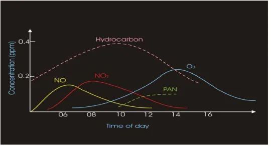
A very important factor is the time of day which affect the amount of photochemical smog present (Figure 2.4).
Early morning traffic increases the emissions of VOCs and NOx when the people
drive to go to work. An oxidation of NO to form NO2.
After that in the morning, traffic dies down and the VOCs and NOx start to react
forming NO2, and increasing its concentration.
When the sunlight becomes more intense later in the day, NO2 amount is broken down
and its by-products form increasing concentrations of O3.
At the same time, few amount of NO2 react with the VOCs and produce toxic
components such as PAN (peroxyacetyl nitrate).
As the sun goes down, there is no production of O3. The O3 that remains in the
atmosphere is then consumed by several different reactions.
Figure 2.4 Diurnal cycle of O3 and its precursors.
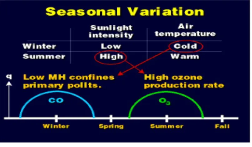
2.4.1.2. Seasonal variation of ozone
The ozone O3 production rate during a seasonal cycle directly relates on the variations in sunlight intensity. Ozone O3 obtains highest levels, and primary pollutants reach low
concentrations when the sun is most intense (i.e., in the summer), On the other hand, there is reduced of o3 production in the winter, when the sun intensity is weak.
Primary pollutants, such as CO, obtain seasonal maxima during the winter. That is because the lower mixing heights during this season in addition to the reduced sunlight intensity. The low mixing heights effect is to reduce the volume of dispersion in which pollutants can mix, which increases the concentration if the source rate is the same.
Figure 2.5 Schematic representation of the seasonal variation of ozone and a primary pollutant (CO).
2.5. Photochemical air quality modelling 2.5.1. Introduction
The large spectrum of atmospheric phenomena describing pollutants dispersion and concentration variate in time from seconds to years and in space scales from meters to thousand kilometers. It is very known to divide the atmospheric phenomena to micro, local, meso and global scale phenomena [J. Fenger, 1999].
Because of the numerous physical and chemical processes happen in the same time, the atmosphere is a very complex system. Measurements of atmospheric and chemical parameters lead to a momentarily view of the atmospheric conditions at a specific time and location. The numerical models allow the study of the atmospheric phenomena and chemical conditions and processes in a full integrated way. Through the spatial and temporal solution of equations describing the combination of all processes inside a model, we can understand each individual process in addition to the interactions between different processes. The best way to understand
and study the atmosphere, is the combined use of state-of-the-art models and state-of the-art measurements.
2.5.2. Air Quality Models
Air quality models represent the good theoretical approach available currently in order to understand the atmosphere variation, and mainly the ozone levels to different air pollution control measures. These models include most of the physico-chemical processes governing formation, transport and fate of photochemical pollutants and allow reproducing and understanding multi-day air pollution episodes [J.Kubler, 2001] (Figure 2.6).
The air quality models inputs can summarised in different groups based on: meteorology, emissions, topography, atmospheric concentrations and grid structure. Using those inputs an air quality model compute the spatial and temporal evolution of air pollutant concentrations, considering the main parameters affecting the pollutants dynamics, such as: diffusion, transport, the chemical and photochemical transformations and dry deposition.
The photochemical air quality model outputs are the resolved air pollution fields in time and space, describing the area response to an emission level. In order to evaluate the model ability to describe well the air pollution dynamics in a selected area, the model results are compared to a good documented historical episode. When the model assessment is finished it can be used to determine the airshed response to different emission control strategies.
2.5.3. Air quality models uncertainties
Even the huge number of developments in numerical field, modelling and simulations of air quality still suffer from many uncertainties due to the large range of scale and the complexity of physico-chemical phenomenon to be considered:
Problem of uncertainties due to initial conditions, a lot of input data are not enough
known like: ozone, VOC and Nox emissions, biogenic emissions, rainfall amount, cloud liquid water content. In addition to meteorological fields, which computed with numerical models that may be uncertain.
Physico-chemical parametrizations produce a high sensitivity to the processing way and
to the parameter values used to represent sub-grid processes.
The numerical algorithms and the discretization can provoke uncertainties, manly for
low resolution because of the computational charge, especially for aerosols.
Even for a validated models, we must keep in mind that the amount of degrees of freedom is large manly in parameterizations, and it is possible to measure only a small number of model outputs. For instance, most of the used chemical transport models have been extensively tuned to meet acceptable model-to-data error statistics for ozone peaks at ground. It does not ensure that the model outputs are satisfactory for 3D fields and other trace substances. There is therefore a problem of applying “overtuned” models, mainly for impact studies or long-term scenario studies (Sportisse, 2007).
2.5.4. Air Quality management
The physico-chemical processes side is not enough to develop an emission control strategy in order to decrease photochemical pollutants ambient concentrations, but also from the technological, social and economical point of view. The air quality management is a complex subject involving diverse topics [J.Kubler, 2001]. A collaboration must be done between the specialists of all topics in order to choose the most acceptable control strategy from a techno-economic and a social point of view. This process shown as a feedback loop in Figure 2.7, first the estimation of temporal and spatial of emission inventory distribution is required in the considered region. The air quality model is then applied to transform the emissions distribution into a pollutant dispersion through numerical simulation of the chemical transformation and physical transport of substances leans on meteorological description of
selected previous episodes. Then the pollutant distribution resulted is evaluated, and if the planned objective is not met, the devloped control strategy is modified taking into account techno-economical feasibility and the political affects, next the new developed emission inventory is tested with the air quality model. This process will repeated until air quality aims are satisfied; regulations are after that considered to meet the emission goal in the control strategy analysis.
Figure 2.7 Diagram of the basic concepts on the role of air quality modelling.
Photochemical models are used in Eulerian, Lagrangian or Hybrid, Eulerian and Lagrangian mode. Lagrangian models describe the motion of an air parcel in the atmosphere and the chemical transformation that happened during the advection. In a Lagrangian model there is no mass exchange between the parcel and its surroundings, except for the emissions that can enter the substance. A Lagrangian model simulates concentrations at various regions and times.
Eulerian models describe the concentration of substance in an array of fixed computational cells. The concentration in an Eulerian model simulated at all locations in function of time. In general Eulerian models are examined that it is technically better and permit comprehensive, explicit processing of physical and chemical treatment. In addition in an Eulerian framework, the interactions of different sources are permitted. These models need good solution methods, using discrete time steps and operator splitting, they use a computational grid which is very cost to apply for a long time. Subgrid resolution can be a limitation because when the size of the grid and the time step areas grid size and time step are
reduced precision increases, in the same time the computation time is increases. Advanced grid models use variable grid spacing or nesting which ameliorates the precision in critical regions and permits the application of cost effective on the atmospheric scales from urban to regional. In a Hybrid model characteristics of Lagrangian types are mixed into an Eulerian framework. These models overcome many of the sub-grid model limitations and many of the prior practical advantages of Lagrangian models, by the development of nested grid resolution and techniques of source apportionment.
Models can also be distinguished according to the computational domain, the model use and duration. Table 2.3 presents different types of models based on the domain size and time scale. The domain of computational consists of cells with specific sizes. The cells size, is the volume in which the components concentration is averaged, determines the spatial resolution of the model. Concerning the resolution in space, with the use of a photochemical model different scales of phenomena can be analyzed.
Table 2.3 Scale definitions and different processes with characteristic time and horizontal scales. (After Atkinson,
2.5.5. 3D Photochemical models requirements
several input parameters are required during the use of a photochemical air quality model, such as meteorological fields parameters: wind speed and direction, humidity, temperature, pressure, stability, substances emissions, in addition to initial and boundary concentration for each components.
Modules used in photochemical model are:
1. Emissions modelling system to create emissions fields for every substances.
2. Meteorological Modelling system to produce meteorological fields.
3. Preprocessors for other initial conditions to the photochemical model.
4. The Air Quality Model.
5. Post-Processors and Visualization.
Figure 2-18 shows a diagram describing the general structure of a photochemical model. The quality of the photochemical model results depend to the initial parameters, the inputs parameters are:
Meteorology: 3-D temperature, winds, humidity, turbulence. Emissions: Temporally and spatially defined.
Topography: Landuse, surface roughness, altitude.
Initial and Boundary Conditions: Gridded array of species concentration for the 1st hour of
the simulation, array of substances concentration for each hour of the simulation at the the domain boundaries.
Photolysis rates file: Photolysis rates for the photochemical reactions in the model.
PHOTOCHEMICAL MODEL
METEOROLOGY
(Wind, temperature, pressure, terrain, precipitation, Humidity etc)
EMISSION INVENTORY PHOTOLYSIS RATES INITIAL CONDITIONS BOUNDARY CONDITIONS PREDICTED CONCENTRATION OF SELECTED POLLUTANTS