Walking and steering control for a 3D biped robot considering ground contact and stability

HAL Id: hal-00794617

https://hal.archives-ouvertes.fr/hal-00794617

Submitted on 26 Feb 2013

HAL is a multi-disciplinary open access

archive for the deposit and dissemination of

sci-entific research documents, whether they are

pub-lished or not. The documents may come from

teaching and research institutions in France or

L’archive ouverte pluridisciplinaire HAL, est

destinée au dépôt et à la diffusion de documents

scientifiques de niveau recherche, publiés ou non,

émanant des établissements d’enseignement et de

recherche français ou étrangers, des laboratoires

Walking and steering control for a 3D biped robot

considering ground contact and stability

Ting Wang, Christine Chevallereau, Carlos Rengifo

To cite this version:

Ting Wang, Christine Chevallereau, Carlos Rengifo. Walking and steering control for a 3D biped

robot considering ground contact and stability. Robotics and Autonomous Systems, Elsevier, 2012,

60 (7), pp.962-977. �10.1016/j.robot.2012.02.007�. �hal-00794617�

Walking and Steering Control for a 3D Biped Robot

Considering Ground Contact and Stability

Ting, Wanga,∗_{, Christine, Chevallereau}a_{, Carlos F., Rengifo}b a

IRCCyN, CNRS, Ecole Centrale de Nantes, 1 Rue de la No¨e, 44321, Nantes, cedex 03,

France b

Universidad del Cauca, Calle 5 No 4-70, Popay´an, Colombia

1. Introduction

The walking of a bipedal robot is composed of different phases such as sin-gle support (SS) with flat foot, SS with foot rotation around the metatarsal axis and double support. During every walking phase there is a dynamic model and a contact with the ground. Thus, an appropriated control law has to be implemented for each phase. Generally, the type of contact with the ground is imposed but it is obtained only if the conditions on ground reaction forces, friction cone and zero moment point (ZMP) are satisfied. The ZMP, firstly in-troduced by Vukobratovic [1], is the most important factor in achieving stable walking of an humanoid robot. The ZMP is defined as a point where the result-ing horizontal reaction moment generated by the ground reaction forces equals to zero. If this point is inside of the support polygon, the robot will not rotate around the edges of its stance foot so it remains flat on the ground. The ZMP can be used to measure instantaneous balance at each time step but it does not contain notion of stability in the future [2].

In earlier studies many bipedal robots adopted a control strategy in which the desired trajectories of joint angles are firstly designed based on the ZMP condition and after that a feedback control tracks the desired trajectories [1]. However, contact conditions could not be satisfied in presence of perturbations.

Most of the recent research on ZMP control can be divided into two general approaches. One method is the periodical replaying of trajectories for the joint motions recorded in advance, like [1], which are then applied to the real robot with a little computed on-line modification [3], [4], [5]. This strategy explicitly divides the problem into subproblems of planning and control. Another method generates a joint-motion in real time, feeding back the present state of the system to be in accordance with the pre-provided goal of the motion, where planning and control are managed in a unified way [6], [7], [8], [9], [10], [11]. Two of the more famous users of these methods are Honda Robot Asimo [3] and Kawada’s humanoid HRP-2 [12], [13].

Almost all of the computed on-line walking controllers are applied to com-pensate the ZMP error. However, the general weakness of the previous methods is that they require considerable experimental hand tuning and the proposed methods are poorly documented. As a preliminary study of our robot, the con-trol law proposed in this paper belongs to the first family of methods. The reference trajectory of the joint angles and ZMP have been computed off-line in [14]. Our first objective is to propose a new control law to satisfy the con-straint of contact and to study the stability of walking, that is, the convergence towards a periodical walking. The computed on-line control modification is not based on experimental tests but on a rigorous stability study.

The proposed control law consists of ZMP controller, swing ankle rotation controller and partial joint angles controller. In the first one, the positions of ZMP in the horizontal plane are regulated to the desired ZMP. This controller creates 2 constraints on joint accelerations and by consequence not all of the joints can track the desired motion. If the obtained joint motion differs from the desired one, a flat-foot impact for the swing foot cannot be assured. In such a case, the stance foot will not be in ”flat-foot-contact” with the sole at the beginning of the next single-support phase. In order to avoid this problem a swing ankle rotation controller is used. In this one, the pitch and roll angle of the swing foot are controlled in order to be equal to their desired values. Like the ZMP controller, the swing ankle rotation controller creates 2 constraints on

joint accelerations. Consequently, for a 3D robot with n actuated joints, n − 4 controlled outputs can be chosen. For simplicity, these n − 4 controlled outputs, which are noted as u, are defined as a linear combination of the n actuated joints. The partial joint angles controller is applied to make u track its desired value ud_{. As a result, the three controllers can offer n dynamic equations to resolve} the acceleration of n actuated joints, then the input torque can be obtained by the inverse dynamics.

It is important to note that in the partial joint angles controller the choice of controlled outputs u depends on the stability analysis of the walking gait under closed-loop control, which is evaluated with the linearisation of the restricted Poincar´e map of the hybrid zero dynamics [15]. In our previous studies [16] and [17], it has been showed through examples, that the choice of controlled outputs will influence the walking stability and with an appropriate selection of these variables a stable walking cycle can be obtained.

In short, the ZMP and swing ankle controllers are used to ensure the stable condition of supported foot and transfered foot respectively. The partial joint angles controller is used to track the reference trajectory and satisfy the stable condition of the overall control law. This control strategy is original for the bipedal robot with feet. Compared to the general control law in recent studies, our control law has some advantages as follows. The proposed method can be viewed as a computed on-line modification of the reference trajectory in order to ensure the satisfaction of the contact constraint. The effect of this modification on walking stability is based on a rigorous stability analysis, and not by testing on the robot which requires considerable experimental hand tuning.

With the proposed control law, the robot can achieve an asymptotically stable and periodic walking along a straight line. The second objective of this paper is adjusting the net yaw rotation of the robot over a step in order to steer the robot along paths with mild curvature. An event-based (or stride-to-stride) feedback controller is appended to distribute set point commands to all the actuated joints in order to achieve a desired amount of turning, as opposed to the continuous corrections used in [18]. This work is an extention from the previous

study for a 3D underactuated bipedal robot [19] and an interesting feature is the ability to control the robot’s motion along paths with mild curvature using only a single predefined periodic motion.

This paper is organized as follows. Section 2 is a description of the biped robot and its dynamic models during different walking phases. Section 3 presents the reference trajectory of the joint angles and ZMP. Section 4 introduces the principle of control law including ZMP controller, swing ankle rotation controller and partial joints controller, and it also introduces the modification of the ref-erence motion after the impact phase to create a continuous and cyclic desired trajectory. In Section 5, the hybrid zero dynamic is explained and stability analysis based on Poincar´e method is proposed. Section 6 gives the comparison of our method with a classical control law for the same robot walking on the rigid ground model and the soft ground model respectively. In Section 7, a supplemental event-based control law used to regulate the walking direction of the robot is presented. Some examples of walking direction control are given. Concluding remarks are made in Section 8.

2. Model 2.1. Biped Model

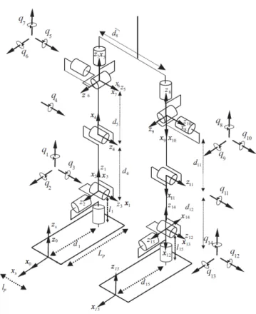
As shown in Fig. 1, the 3D robot is comprised of a torso and two identical legs that are independently actuated and terminated with flat-feet. Each hip and ankle consists of a revolute joint with 3 DOF and the knee is a 1 DOF revolute joint, and each DOF is independently actuated. As a result, it has 14 DOF in the single support phase and 14 actuators. The vector q = [q1, . . . , q14]T contains the relative joint positions of the biped, and the torques are grouped into a torque vector, Γ = [Γ1, . . . , Γ14]T, where qj, j ∈ (1, . . . , 14) corresponds to the rotation about zj. It’s worth noting that the coordinate system x0y0z0 is fixed on the support foot while the coordinate system xsyszs is fixed on the ground and it is called the absolute coordinate system. The origins of them are the same only during the first walking step.

Figure 1: Biped Model

The length and mass of each body are given in Table 1 and Table 2. All links are assumed to be massive and rigid. The inertia of the links is also taken into account, and other parameters of the robot in detail are shown in [14].

Table 1: length parameters(m)

d1, d15 d4, d12 d5, d11 d8 l1, l15 lp Lp 0.185 0.392 0.392 0.190 0.05925 0.08 0.207

Table 2: mass parameters body f oot shin thigh torso

2.2. Dynamic model

The walking gait consists of single support phases where the stance foot is flat on the ground separated by impacts, that is, instantaneous double support phases where leg exchange takes place. The dynamic models for every walking phase are derived here by assuming support on right leg, which is noted as leg 1. They are described as follows, and the models for support on leg 2 can be written in a similar way.

2.2.1. Dynamic model of single support phase

The Newton Euler algorithm presented in [20] is used to calculate the dy-namic model of 3D biped robot during the single support phase [14]. The ac-tuator torques and the ground reaction (forces and torques) to the stance foot can be computed as soon as the joint position, velocity and acceleration q, ˙q, ¨q are known, and they are linear functions of the acceleration ¨q. Consequently, the dynamic model is represented as:

     F M Γ      = N E(q, ˙q, ¨q) = N E1(q)¨q + N E2(q, ˙q) (1)

N E1(q) being the positive definite inertia matrix of the robot and N E2(q, ˙q) a vector containing the gravitational, Coriolis and centrifugal forces. F and M compose the wrench vector exerted by the ground on the stance foot. Both quantities are expressed in the reference frame x0y0z0and they will be used to calculate the position of ZMP. The calculation of the torque vector Γ will be used in the control law.

2.2.2. ZMP dynamics

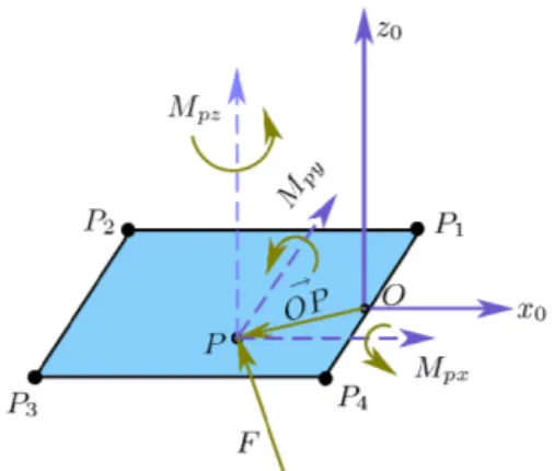
When leg-1 is on the ground, a ground reaction force and moment can be expressed about any point in the support plane. If a point P is in the plane of the foot-1 (see Fig. 2), the ground reaction moment Mp of P can be calculated by:

Mp= M − →

Figure 2: The support foot

where →

OP is the distance vector of the point P in the reference frame x0y0z0. Considering F, M are functions of q, ˙q, ¨q and linear functions of the acceleration ¨

q (see (1)), the components of Mpalong the axes x0 and y0 can be written as:   Mpx Mpy   = f (q, ˙q, ¨q, → OP ) = W ¨q + H (3)

where the function f () in (3) depends on (1) and (2), and W , H can be obtained by: H = f (q, ˙q, ¨q = 014×1, → OP ), (4) and W (:, i) = f (q, ˙q, ¨q = ei, → OP ) − H (5) e_i being the column i of an identity matrix of dimension 14. According to the definition of zero moment point (ZMP), if P is ZMP, the horizontal ground reaction moment of the ground reaction force about this point equals to zero. Thus (3) can be used to constrain the ZMP which is such that:

Mpx= Mpy = 0 (6)

to be a desired point P which is time-varying and depends on the precomputed reference trajectory [1].

2.2.3. Dynamic model of impact phase

An impact exists at the end of the single support phase. After that, the legs swap their roles from one step to the next. Considering the robot is symmetric, we only study a single step to deduce the complete behavior of the robot over a sequence of steps on alternating legs. During the impact, the biped’s config-uration variables do not change, but the generalized velocities undergo a jump. As shown in [15], this jump is linear with respect to the joint velocity before the impact. The moments just before and after impact are denoted by − and + respectively, the impact model can be written as (see [14]):

   q+= E · q− ˙q+= E · I(q− ) · ˙q− (7)

where E is the permutation matrix describing leg’s exchange and I(q− ) repre-sents the linear jump of the joint velocity after impact.

3. The reference trajectory

Starting from a reference trajectory of joint angles described as function of time qd_{(t) which has been calculated off-line through the minimization of the} energy consumption in [14], a new parametrization is proposed. Here and in the following subsections the superscript d denotes the desired value. Function qd_{(t) is parametrized by a quantity depending on the state of the robot that is} strictly monotonic like time t during a complete walking phase of one step. By using this method, only the kinematic evolution of the robot’s state is regulated but not its temporal evolution. This means the control law is defined to follow a joint path but not a joint motion. It was used successfully for the walking of bipeds with point feet [21], [22], [23], [16] and the walking of planar biped with foot rotation [24]. Especially in [24], this method allows the simultaneous control of the joint path and the ZMP. Therefore, it is still used for the 3D biped robot with flat feet. The parametrized reference trajectory is given as follows.

In a forward walking motion, the x-coordinate of the hip increases monoton-ically. Hence, if the virtual stance leg is defined by the line that connects the

xs

zs

q3

q4

θ

Figure 3: The definition of θ.

stance foot to the stance hip, the angle of this leg in the sagittal plane, denoted by θ, is monotonic and it can replace the time t to parametrize qd _{and ZM P}d_. As shown in Fig. 3, the shin and the thigh have the same length, thus θ can be computed by:

θ = q3+ q4/2. (8)

Then the reference path written as hd_{(θ) is such that:}          qd_{(t) = h}d_(θ) ˙qd_{(t) =}∂hd_(θ) ∂θ ˙θ ¨ qd_{(t) =}∂2 hd_(θ) ∂θ2 ˙θ2+ ∂hd_(θ) ∂θ θ¨ (9)

where hd_{(θ) is designed in order to be compatible with a periodic solution of} the biped model. According to a known reference trajectory qd_{(t), ˙q}d_{(t), ¨q}d_(t), in (9) hd_(θ), ∂hd_(θ)

∂θ and ∂2

hd_(θ)

∂θ2 can be deduced and they are assumed to be known in the following contents. Similarly, for every qd_{(t), there is a correspond} θ and ZM Pd_{(t), then the desired ZMP can be described by θ and it is written} as: ZM Pd_(θ).

4. The proposed control law

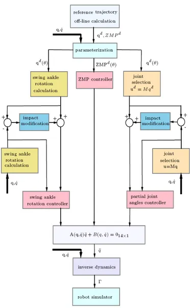
As shown in Fig. 4, the overall control law consists of ZMP controller, swing ankle rotation controller and partial joint angles controller. The former two

controllers are used to achieve ZM P = ZM Pd_{(θ) and make the swing foot} keep flat at impacts respectively, which are helpful to insure the stable contact. The third controller implements the joint path control and it is partial since some contraints on torques are imposed by the former two controllers.

4.1. ZMP controller

The objective of this controller is to have:

ZM P = ZM Pd(θ). (10)

ZMP tracking can be quite conservative but insure to avoid unexpected rotation of the stance foot. Another posibility is to limit the minimal and maximal values of ZMP [25]. According to the definition of ZMP, if P in Fig. 2 is ZMP, (3) can be rewritten as:

W (q, ˙q)¨q + H(q, ˙q) = 02×1 (11)

where W and H are recalculated by (4) and (5) with →

OP = ZM Pd_{(θ). This} equation clearly shows that the acceleration ¨q must satisfy two constraints to produce ZM P = ZM Pd_(θ).

4.2. Swing ankle rotation controller

With the reference trajectory qd_{, ˙q}d_{, ¨q}d_{, the sole of the transfered foot} par-allels to the ground at each impact phase. As stated in the Introduction, this controller is necessary because not all of the joint angles q are controlled. We propose to control the orientation of the swing foot in the frontal and sagittal plane such that the robot will touch the ground with flat foot and to insure that the next impact will occur in a good way.

As shown in Fig. 1, the angle q14 is the rotation angle of the 14th joint around the axes z14. It only affects the yaw motion of the swing foot, so only the previous 13 joints are constrained. Defines_R

13, the 3 × 3 orientation matrix from the coordinate system xsyszs to x13y13z13 :

s_R 13= h s n a i , (12)

where s3×1, n3×1 and a3×1 are unitary vectors defining x13y13z13 in framesR respectively, and they only depend on the first thirteen joint angles of q, exactly, q1, q2, . . . , q13. Using the reference trajectory qd, we define sRd13 = [sd, nd, ad] to denote the desired orientation of transformation matrixs_R

13. If there exists tracking error between q and qd_{, there will be small error in the orientation of} the swing ankle which can be defined as ξ [26]:

ξ =1 2(s × s

d_{+ n × n}d_{+ a × a}d_{). (13)}

The derivatives of the orientation error are :    ˙ξ =s_ω 13d−sω13 ¨ ξ =s_˙ω 13d−s˙ω13 (14) wheres_ω

13ands˙ω13are the angular acceleration and velocity of the joint 13 in the absolute coordinate system xsyszs. sR13,sω13 ands˙ω13 in (12) can be effi-ciently computed by the forward recursive equations of the general serial robot with q1, . . . , q13, their velocity and acceleration [20] (see Appendix Appendix A).

Because the orientation in the frontal and sagittal plane of the swing foot doesn’t depend on the rotation components around zsaxis (see Fig. 1), only the first two components of ξ have to be regulated to zero:

ξxy = 02×1 (15)

Here and in the following subsections the subscript xy denotes the first two lines of the vector, which correspond to the rotation around xsdirection and ys direction respectively. (15) can be achieved by the PD controller:

¨ ξxy+ K1 ε ˙ξxy+ K2 ε2 ξxy= 02×1. (16)

with K1> 0, K2> 0, and ε > 0. The above equation imposes two constraints on q, ˙q and ¨q. Such constraints read as:

Ws(q, ˙q)¨q + Hs(q, ˙q) = 02×1. (17) where Ws(q, ˙q) denotes all the coefficient terms of ¨q and Hs(q, ˙q) denotes all the terms without ¨q in (16). The detail is presented in Appendix Appendix B.

4.3. Partial joint angles controller

Besides of the former two controllers, the control law is also designed to track the joint reference path qd_{= h}d_{(θ). However, (11) and (17) have offered 4} restrictions about the states of robot q, ˙q, ¨q, so we can’t control q = qd _directly and we can only choose 10 targets to track with. Thus, how to choose 10 controlled outputs from 14 actuated joints is presented at first.

From the principle of swing ankle rotation controller, we know that the pitch and roll angle of the swing foot are constrained to be their desired values. It means that 2 joint angles can be determined by the other 11 joint angles in q1, q2, . . . , q13 according to the definition of ξxy in (12) and (13).

Because the swing ankle is actuated by the 12th _{and 13}th _{joint (see Fig. 1),} so we can suppose that q12and q13have been defined according to q1, q2, . . . , q11. Thus there is no need to consider them again in the partial joint angles con-troller. In addition, section 3 has presented that all the reference trajectory are parametrized by θ and θ = q3+ 0.5q4, so q3and q4are not independent of each other and q3 is excluded here. Therefore, the independent joint angles are:

Qr= [q1, q2, q4, . . . , q11, q14]T11×1 (18) Qr has 11 elements but only 10 controlled outputs can be defined. Since the second joint influences the position of ZMP in the frontal plane directly, in order to distinguish q2 from other joints in Qr and avoid singularity, the controlled joint angles are chosen as:

u = Q + M1q2 (19)

with

Q = [q1, q4, . . . , q11, q14]T. (20) Where M1is a 10×1 constant matrix to be determined by the stability analysis. The next section will show that the choice of M1affects the stability of the robot, in the sense of the convergence toward cyclic motion. The stability condition will be a criteria used to select M1.

Next, the objective of this controller is to regulate u to track its desired value ud_{(θ). It is achieved by a PD control:} ¨ u − ¨ud₊Kd ε ( ˙u − ˙u d_{) +}Kp ε2 (u − u d_{) = 0} 10×1, (21)

where ud_{, ˙u}d_{, ¨u}d _{can be calculated using the definition of u in (19) and the} referenced trajectory qd_{, ˙q}d_{, ¨q}d _{in (9). Because the controlled partial joint} angles u is a linear function of the joint angles q (see (19)), obviously, ¨u in (21) is a linear function of ¨q, so (21) can be written as the same format as (11) and (17):

Wj(q, ˙q)10×14q + H¨ j(q, ˙q)10×1= 010×1, (22) where Wj(q, ˙q) denotes all the coefficient terms of ¨q and Hj(q, ˙q) denotes all the terms without ¨q in (21).

It is worth mentioning that if u = ud_{(θ), according to (19), Q is such that:} Q = Qd_{− M}

1(q2− qd2). (23)

(23) implies that this controller can also be regarded as an on-line modification of the joint reference motion, which is like many existent methods. However, the advantage of our controller is that the effect of this on-line modification (or the choice of M1 in (23)) on stability will be studied.

4.4. Modification of the tracked errors caused by impact

Based on the proposed three controllers, the desired properties respectively

are: _         y1= ZM P − ZM Pd(θ) = 0 y2= ξxy= 0 y3= u − ud(θ) = 0 (24)

These controllers act only in the single support phases. The original reference trajectory is defined by taking into account the impact phase. The impact con-dition is a geometric concon-dition. Thus, it can occur with some errors, especially with some errors on θ and q2 because they are not controlled directly as other states in u. As a result, large errors on the joint position and velocity will be created after impact, that means discontinuity of errors will exist.

In order to avoid the discontinuity, the reference trajectory in (24) are mod-ified stride to stride so that they are compatible with the initial state of the robot at the beginning of each step [16]. It is not necessary to modify ZM Pd_(θ) because the position of ZMP acts directly at the acceleration level where the discontinuities are acceptable. The new output for the feedback control design

is: _         y1= ZM P − ZM Pd(θ) = 0 y2c= ξxy− ξxyc= 0 y3c= u − ud(θ) − uc= 0 (25)

Here ξxyc and uc are modification terms of the original reference motions. The calculation of them is presented as follows.

The function ucis taken to be a four-order continuously differentiable poly-nomial function of θ:

uc= a0+ a1θ + a2θ2+ a3θ3+ a4θ4, (26) where the coefficients a0, . . . , a4 are defined such that1

         uc(θi) = y3i ∂uc ∂θ(θi) = ˙ y3i ˙ θi uc(θ) ≡ 0, θ ≥ θi+θ₂ f. (27)

where y3i and ˙y3i denote the initial values of y3 and ˙y3, and they are updated at the beginning and held constant throughout the step. Specifically, y3i = ui− ud(θi) and ˙y3i= ˙ui− ˙ud(θi). Here θi and θf are the initial and final value of θ from qi to qf respectively, and they can be calculated by (8).

As shown in Fig. 19, by using uc defined in this way the new reference trajectory starting from the current state just after the impact are smoothly joined to the original reference trajectory at the middle of the step. In particular, for any initial error, the initial reference trajectory ud _{is not modified in the} second part of the step : θ ≥ θi+θf

2 .

1_{The four order polynomial is used for θ}

i≤ θ ≤

θi+θf

2 ; Continuity of position, velocity

and acceleration is ensured at θ =θi+θf

Similarly, the function of ξxycin (25) is defined as the same format as (26) and all the coefficients are determined using the value of y2 in (24) and its derivative at the beginning of each step. As a result, these modification terms are supplemented in the PD control expressions (16) and (21):

¨ ξxy− ¨ξxyc+ K1 ε ( ˙ξxy− ˙ξxyc) + K2 ε2 (ξxy− ξxyc) = 02×1 (28) ¨ u − ¨ud_{− ¨u} c+ Kd ε ( ˙u − ˙u d_{− ˙u} c) + Kp ε2(u − u d_{− u} c) = 010×1 (29) 4.5. Torque calculation

With the proposed three controllers, 14 equations about q, ˙q, ¨q are obtained by (11), (17) and (22), and they are affine functions of ¨q. Considering the impact modifications, the latter two controllers (17) and (22) are recreated using (28) and (29) to satisfy (25), and they are also affine functions of ¨q. Thus, 14 new equations about q, ˙q, ¨q can be combined as:

A(q, ˙q)¨q + B(q, ˙q) = 014×1, (30) Next, the ¨q is resolved directly:

¨

q = −A−1_{B (31)}

Then, the desired torques Γ can be calculated with ¨q, ˙q and q by the inverse dynamics via Newton Euler algorithm (1).

5. Stability analysis

The stability of the control law is defined in the sense of the convergence toward a periodic motion. As proposed in [21], [22], [23], [16] and [15, Chap. 4], the stability of the closed-loop system can be studied in a reduced-dimensional state space based on Hybrid Zero Dynamics (HZD). For a system modeled by ordinary differential equations (in particular, without impact dynamics), the maximal internal dynamics of the system that is compatible with the output being identically zero is called the zero dynamics [27], [28]. HZD is a zero dynamics of the full hybrid model, i.e., the dynamics at impact is included.

Next we will present how to study the stability of the closed-loop system in a reduced-dimensional state space.

5.1. Using HZD to obtain reduced-dimensional states

According to the definitions of HZD, the controller with impact modifications (11), (28) and (29) creates the HZD, with which the behavior of the robot is completely defined by the impact map and the swing phase zero dynamic model (25). The stability analysis of walking can be obtained by using the Poincar´e method. Different Poincar´e section can be considered. Here it is chosen at θ = 0.4θi+0.6θf. At this instant the swing foot has not yet touched the ground, and since θ ≥ θi+θf

2 the values of the controlled variables u and ξxy are not affected by ucand ξxyc(see Fig. 19). A restricted Poincar´e map is defined from Sθ∩Z to Sθ∩ Z, where Z = {(θ, q, ˙q)|y1= 0, y2c = 0, ˙y2c = 0, y3c = 0, ˙y3c= 0} describes the zero dynamics manifold (see (25)) and Sθ = {(θ, q, ˙q)|θ = 0.4θi+ 0.6θf} is the Poincar´e section. The key point is that the state of the robot can be parametrized by three independents variables x = [q2, ˙q2, ˙θ]T in Sθ∩ Z. The reduction of the states dimension is explained as follows.

In Sθ∩ Z, from the third line of (25), the definition of u in (19) and uc in (27), we have:

Q = ud(θ) − M1q2. (32)

It shows Q is determined by θ, q2and M1. The second line of (25) and the defini-tion of ξxyin (12), (13) show that q12and q13can be calculated by q1, q2, . . . , q11. In fact, according to the definition of Q and θ (see (20), (8) and (32)), we can deduce that q12 and q13 depends on q2, θ and M1. Thus the calculation of q12 and q13 can be denoted as a function fq():

[q12, q13] = fq(q2, θ, M1). (33) (20) and (8) show that there exists a linear relation between q and Q, q12, q13, θ, q2:

q = Mh[Q, q12, q13, θ, q2]T14×1 (34) where Mh is a 14 × 14 constant matrix.

Therefore, (34) shows the full state of the robot q is determined by q2, θ and M1. Consequently, a simplified expressions of q, ˙q is defined as:

[q, ˙q] = fHZD(q2, θ, ˙q2, ˙θ, M1, Cqd) (35) where Cqd denotes all the known terms such as the reference trajectory qd and its derivatives.

In consequence the acceleration ¨q can be expressed as function of q2, θ, ˙q2, ˙θ, ¨q2, ¨θ and it depends on M1 and Cqd. Thus (25) corresponds to:

         WHZD(q, ˙q)   ¨ q2 ¨ θ  + HHZD(q, ˙q) = 02×1 [q, ˙q] = fHZD(q2, θ, ˙q2, ˙θ, M1, Cqd) (36)

where the first line of (36) is deduced by the ZMP controller (11). WHZD(q, ˙q) denotes all the coefficient terms of ¨q2 and ¨θ, and HHZD(q, ˙q) denotes all the terms without these terms.

Obviously, with definition of HZD, the first line of (36) can replace the original resulted dynamic equation (30) to describe the behavior of the robot from the Poincar´e section until the impact. Just before the impact the complete states of the robot are calculated by using the second line of (36). Then the model of impact is used and uc, ξxyccan be calculated. The behaviour of the robot from the beginning of the next step to the Poincar´e section is then calcu-lated by equation of HZD that is similar to (36) but includes the modification terms of the reference trajectory uc, ξxyc.

5.2. Stability analysis at a fixed-point

The known cyclic motion qd_{(θ) gives a fixed-point x}z∗_{= (q}

2d(θ∗), ˙qd2(θ ∗

), ˙θ∗ ) for the proposed control law for any value of M1, where θ∗= 0.4θi+ 0.6θf.

The restricted Poincar´e map Pz_{: S}

θ∩ Z → Sθ∩ Z induces a discrete-time system xk+1= Pz(xk). [29] states that, for ε sufficiently small in (28) and (29), the linearization of Pz _{about a fixed-point determines exponential stability of} the full order closed-loop robot model. Define δxk = xk− x∗, the Poincar´e map

linearized about the fixed-point x∗

gives rise to a linearized system,

δxk+1= Azδxk, (37)

where the (3 × 3) square matrix Az _{is the Jacobian matrix of the Poincar´e} map, and it can be calculated as shown in [16]. A fixed-point of the restricted Poincar´e map is locally exponentially stable, if, and only if, the eigenvalues of Az _{have magnitude strictly less than one [15, Chap. 4].}

6. Examples

(36) shows that the dynamic property of the system is influenced by the choice of M1, exactly, the choice of joint angles to be controlled or the modifi-cation of reference motion (see (23)). One objective of this part is to study the influence of choice of M1on the stability and to obtain some M1to stabilize the walking. The other objective is to compare the robustness of our control law with that of a classical method.

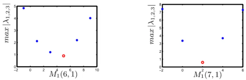
6.1. The effect of different controlled partial joints on the walking stability An exploration technique is used to illustrate the effect of the choice of M1. First, arbitrary 9 components of M1are fixed to zero, then the largest magnitude of the eigenvalues of Az _{are drawn as function of the 10}th _{component of M}

1. If they are less than 1, the resulted walking is stable. The analysis results of M1(j, 1), j = 6, 7 are shown in Fig. 5, where the red circles denote the largest magnitude of eigenvalues of Az _{is less than one, that means the stable} cases exist. It also shows that the eigenvalues of Az _{are large than 1 when} M1 = 010×1, that means the walking is not stable. In fact, in this case the controlled joint angles are u = [q1, q4, . . . , q11, q14]T (see (19)) and the reference motion Qd _{is not modified by the tracking error of q}

2(see (23)).

6.2. The robustness of the control law with M1(6, 1) = 5 for the rigid ground model

According to Fig. 5, when we choose M1(6, 1) = 5, the walking should be stable. In order to prove the validity and superiority of our control law, an

−2 0 2 4 6 8 10 0 1 2 3 4 5 m a x |λ 1 ,2 ,3 | M1(6, 1) −2 0 2 4 6 0 1 2 3 4 5 6 7 8 m a x |λ 1 ,2 ,3 | M1(7, 1)

Figure 5: max |λ1,2,3| versus M1(j, 1), j = 6, 7, when the other 9 components of M1 are zero.

example of this stable walking case is compared with a classical control law, in which all the joint angles are controlled and the desired properties of the closed loop system is:

¨

q = ¨qd− Kd( ˙q − ˙qd) − Kp(q − qd), (38) where Kd > 0 and Kp > 0. The joint torques can be obtained by (1) using q, ˙q and ¨q. Next, the same reference trajectory, the same simulator of the robot and the same simulation parameters are used for the two control laws. For the control law (38), in order to limit the influence of errors at the beginning of the step, the reference trajectory in (38) is also modified as presented in section 4.4. Computation of impact and contact forces between foot and ground is an es-sential task for the simulation of a bipedal robot walking cycle. In our simulator, foot is supposed rigid and composed of four contact points P1, P2, P3 and P4 (see Fig. 2). If one of these points is in contact with the ground the correspond-ing reaction force is computed by solvcorrespond-ing a linear complementarity problem (LCP) [30]. Since the punctual contact at each corner of the foot P1, . . . , P4 is considered, the slipping, rolling or take-off of the foot can be modeled. An initial error of 0.01rad is introduced on q2 and a velocity error of 0.01rad/s is introduced on ˙q2 and ˙θ, the errors on the other joints are introduced to have a double support configuration.

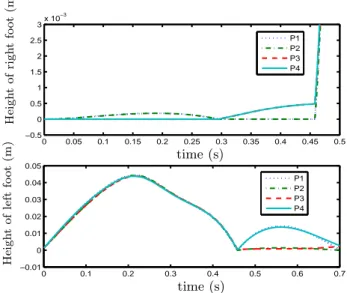
The flat rigid ground model is used at first. For the proposed control law since the ZMP is controlled, the position of ZMP can track its desired value ZM Pd _{as shown in Fig. 6, thus the stance foot can remain flat on the ground}

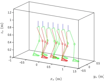
during single support phases. Moreover, it has been presented that the trans-fered foot is flat at each impact phases with the reference trajectory, that means the height of four points P1, P2, P3 and P4 of the swing foot are the same. Thanks to the swing ankle rotation controller, this condition is satisfied al-though not all the joint angles q are controlled to track qd _{in the design of the} overall control law, see Fig. 7. It describes the height of four points P1, . . . , P4 for two feet respectively and it shows that the traces of P1, . . . , P4are almost the same, that means the supported foot remains flat on the ground and the swing feet is also flat before impact as prescribed for the reference motion, which can validate the swing ankle rotation controller. The walking motion of first three steps is shown in Fig. 11, it also displays the stable walking is achieved. The evolution of the error on q2(the joint not directly controlled) is shown in Fig. 10. At the beginning the error increases to satisfy the condition on the ZMP but after that and step by step this error decreases and the cyclic desired motion is reached.

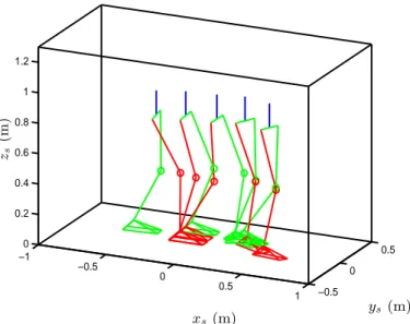
On the contrary, for the classical control law, since all the joint angles are controlled, the tracking error of the joint is close to zero at the end of the step (see Fig. 10, for the joint angle q2). However, the initial error is so high that the ZMP reaches the limits along the axis y as shown in Fig. 9. As a result, the stance foot rotates about its edges as displayed in Fig. 8. Fig. 12 also shows that the height of hips changes irregularly and the robot will fall down.

The comparison reconfirms that the control of ZMP is much more important than the tracking of predefined joints trajectory. It also indicates that the swing ankle rotation controller is helpful to the stable contact with the ground. In addition, the obtained stable walking shows that the choice of controlled partial joints using the stability analysis is effective.

6.3. The robustness of the control law with M1(6, 1) = 5 for the soft ground model

In order to further test the proposed control law, now a soft ground model is used in the simulator [31]. Obviously, it will propose higher requirements for the control law.

Figure 6: Position of ZMP in the foot sole with the proposed control law using the rigid ground model: it tracks its desired value and moves periodically.

0 1 2 3 4 5 0 0.02 0.04 0.06 0 1 2 3 4 5 0 0.02 0.04 0.06 time (s) time (s) H ei g h t o f ri g h t fo o t (m ) H ei g h t o f le ft fo o t (m )

Figure 7: Height of feet with the proposed control law using the rigid ground model.

0 0.05 0.1 0.15 0.2 0.25 0.3 0.35 0.4 0.45 0.5 −0.5 0 0.5 1 1.5 2 2.5 3x 10 −3 0 0.1 0.2 0.3 0.4 0.5 0.6 0.7 −0.01 0 0.01 0.02 0.03 0.04 0.05 P1 P2 P3 P4 P1 P2 P3 P4 time (s) time (s) H ei g h t o f ri g h t fo o t (m ) H ei g h t o f le ft fo o t (m )

Figure 8: Height of feet with the classical control law, for the right foot a zoom is done along the vertical axis to show the unexpected rotation of the stance foot. 0 0.1 0.2 0.3 0.4 0.5 0.6 0.7 −0.25 −0.2 −0.15 −0.1 −0.05 0 0 0.1 0.2 0.3 0.4 0.5 0.6 0.7 −0.05 0 0.05 right foot left foot right foot left foot time (s) time (s) Z M Px (m ) Z M Py (m )

0 1 2 3 4 5 −1.6 −1.4 −1.2 −1 −0.8 −0.6 −0.4 −0.2 0 0.2 0.4 time (s) ∆ q2 (d eg re e) 0 0.2 0.4 0.6 0.8 −0.6 −0.5 −0.4 −0.3 −0.2 −0.1 0 0.1 ∆ q2 (d eg re e) time (s)

Figure 10: The tracking errors of q2with an initial error for the proposed control law (left figure) and the classical method (right figure) for several steps.

−1 −0.5 0 0.5 1 1.5 −0.5 0 0.5 0 0.2 0.4 0.6 0.8 1 1.2 xs (m) zs (m ) ys (m)

Figure 11: The walking motion of first three steps with the proposed control law.

−1 −0.5 0 0.5 1 −0.5 0 0.5 0 0.2 0.4 0.6 0.8 1 1.2 xs(m) zs (m ) ys (m)

Figure 12: The walking motion of first two steps with the classical control law.

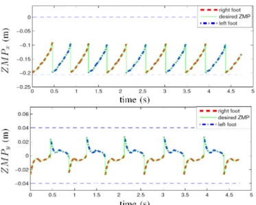
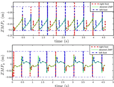
The same initial errors are introduced to every joint position and velocity as presented in the previous subsection. Since the soft ground model is used, the ground reaction force (GRF) changes acutely at the impact moment (see Fig. 13). As a result, ZMP is out of the polygon of support foot, but it is controlled quickly after the impact, as shown in Fig. 14. Consequently, the height of stance foot and the tracking error of q2 shake a little in the beginning of swing phase but at once recovers to zero (see Fig. 15 and Fig. 16). On the contrary, the walking is not stable with the classical control law. The results are similar to that using rigid ground model in Fig. 8 and Fig. 9 so they are not shown here.

7. Steering control

With the proposed control law, the robot can achieve an asymptotically stable and periodic walking along a straight line. It can be observed that the walking motion is not exactly along the x-axis with initial error. However, the robot is expected to be able to move all over the working place when it works in human environment. Thus we need the precise steering control not only the

0 0.5 1 1.5 2 2.5 3 3.5 4 4.5 0 200 400 600 0 0.5 1 1.5 2 2.5 3 3.5 4 4.5 0 200 400 600 time (s) time (s) G R F o n th e ri g h t fo o t (N ) G R F o n th e le ft fo o t (N )

Figure 13: Ground reaction force (GRF) of the soft ground model.

0 0.5 1 1.5 2 2.5 3 3.5 4 4.5 5 −0.25 −0.2 −0.15 −0.1 −0.05 0 0 0.5 1 1.5 2 2.5 3 3.5 4 4.5 5 −0.04 −0.02 0 0.02 0.04 right foot desired ZMP left foot right foot desired ZMP left foot time (s) time (s) Z M Px (m ) Z M Py (m )

Figure 14: Position of ZMP in the feet sole with the proposed control law using the soft ground model: it moves periodically and returns to the limits fast after impact.

0 0.5 1 1.5 2 2.5 3 3.5 4 4.5 −0.01 0 0.01 0.02 0.03 0.04 0.05 0 0.5 1 1.5 2 2.5 3 3.5 4 4.5 −0.01 0 0.01 0.02 0.03 0.04 0.05 time (s) time (s) H ei g h t o f ri g h t fo o t (m ) H ei g h t o f le ft fo o t (m )

Figure 15: Height of feet with the proposed control law using the soft ground model. 0 1 2 3 4 5 6 −1.6 −1.4 −1.2 −1 −0.8 −0.6 −0.4 −0.2 0 0.2 0.4 time (s) ∆ q2 (d eg re e)

Figure 16: The tracking errors of q2 with the proposed control law using the soft ground model.

walking straight simply. Therefore, the objective of this section is adjusting the net yaw rotation of the robot over a step in order to steer the robot to walk along paths with mild curvature.

There are few studies about direction control. [32] and [33] studied the turning motions for biped with ZMP-based footstep planning. [34] proposed the robust direction control system that used gyro sensor feedback under envi-ronment with disturbance. In [35], motion stability during turning is ensured by adjusting the swing leg center of mass (COM) and hip position trajectories in a trial and error fashion. In this paper, an event-based feedback controller [36] is integrated with the proposed control law in Section 4 to regulate the walking direction through the net yaw motion about the stance foot over a step. Differ-ent from the previous studies, in our approach, the stability during steering is maintained. In addition, an interesting feature of this work is that one is able to control the robot’s motion along a path with limited curvature using only a single predefined periodic motion.

7.1. Stability analysis of the yaw motion

In order to describe the yaw motion of the robot, the walking direction angle q0 is supplemented to the configuration variables of the robot, that is: qe _{= [q}T_{, q}

0]T. As shown in Fig. 17, ql and qr are respectively defined as the direction angle relative to xs-axis of left foot and right foot respectively, the walking direction angle of the whole body q0 is given by:

q0= ql+ qr

2 . (39)

Where qland qrcan be obtained using the position of two feet in the xsysplane of the absolute frame.

Next, the stability of the extended system can be studied as shown in sub-section 5.2. With the proposed control law, the behavior of the robot can be studied in the HZD. The extended states xe _{= [q}

2, ˙q2, ˙θ, q0]T is used and the corresponding linearized extended restricted Poincar´e map at the fixed-point based on (37) is written as:

δxe

Figure 17: Description of walking direction

where Ae _{is a 4 × 4 matrix and δx}e

k = xek− xe∗. According to the linearization method of the Poincar´e map about the fixed-point [16], Ae_{can be described as:}

Ae=   Ae δxk,xk+1 A e δq0 k,xk+1 Ae δxk,q0 k+1 A e δq0 k,q0 k+1   (41)

where the four components of Ae _{denote the effect of introduced errors δx} k or δq_0k on the states of the next step xk+1 or q0k+1 respectively. Obviously, Ae

δxk,xk+1 = A

z_{, which has been obtained in subsection 5.2. Moreover, the} impact surfaces and the dynamic model are invariant under the rotation around the zs-axis of the absolute frame [37]. Therefore, during the complete walking phase, a perturbation on q0is conserved after one step and it doesn’t affect the configuration of the biped. As a consequence the resulted Ae _{is rewritten as:}

Ae₌   Az ₀ 3×1 Ae δxk,q0 k+1 1   (42)

Since the stability of the extended system is determined by the eigenvalues of Ae_{, in which the first three eigenvalues are the eigenvalues of A}z_{and the fourth} eigenvalue is 1, that means the extended system is not stable, exactly, the yaw motion is not stable so the walking direction angle q0 can not be controlled by the control law proposed in Section 4.

7.2. Stabilization of the yaw motion

In order to stabilize the yaw motion, all the eigenvalues of Ae _{in (42) must} be less than 1. Here an event-based feedback control [36] is introduced to

−1 0 1 2 3 4 5 6 −0.4 −0.35 −0.3 −0.25 −0.2 −0.15 −0.1 −0.05 0 0.05 0.1 xs(m) ys (m )

Figure 18: The positions of the feet at impacts with initial error of states, where the red points denote the midpoint of two feet. The robot departs the direction of xs axis.

modify the the eigenvalues of Ae_{. Because the ZMP control and the swing} ankle rotation control are always desired, so the event-based feedback control is only supplemented to the partial joint angles controller, then the desired property of the overall controller shown in (25) is rewritten as:

         y1= ZM P − ZM Pd(θ) = 0 y2c= ξxy− ξxyc= 0 y3cs= u − ud(θ) − uc− us= 0 (43)

where the supplemented term us is defined as uc in (26)

us= b0+ b1θ + b2θ2+ b3θ3 (44) with b0, b1, b2, b3defined such that:

   us(θf) = β us(θ) ≡ 0, θ ≤ θs and θ∗≤ θs< θf. (45)

where β is the feedback control term to be determined, and it is retained con-stant during the swing phase and updated at each impact. θ∗

is the selected fixed-point in subsection 5.2 (θ∗

Poincare Section ud_(θ i) u(θi) ud ud+ uc ud+ uc+ us θ θi θi+θ₂ f θ∗ θf β

Figure 19: The modification of the reference path ud_.

moment of the event-based feedback control and it is limited by θ∗

≤ θs < θf to insure that the state of the robot is completely defined by xe_{in the Poincar´e} section. In order to obtain sufficient time to control the walking direction before impact, here we choose θs= θ∗. By introducing uc and usto ud, the resulted reference trajectory can be described by Fig. 19. It should be noted that uc modifies only the first part of the stance phase ( uc= 0 when θ ≥ θi+θ₂ f), and usmodifies only the last part of the stance phase (us= 0 when θ ≤ θs). There-fore, the choice of usin (45) is convenient because it does not require a re-design of the controller that created the HZD. The Poincar´e map can now be viewed as a nonlinear control system on Sθ∩ Z with inputs βk, namely xek+1= Pz(xek, βk), where βkis the value of β during the step k. Linearizing the Poincar´e map about the fixed-point xe∗ _{and the nominal parameter value β}∗

= 010×1 leads to δxek+1= Aeδxek+ F δβk, (46) where δβk = βk− β∗ and F is the Jacobian matrix of Pz with respect to β. Designing a feedback matrix

δβk = −Kδxek (47)

such that the eigenvalues of (Az_{− F K) are strictly less than one will} exponen-tially stabilize the fixed-point xe∗_.

(10 × 4) gain matrix K is calculated via DLQR technique so that the state-feedback control law (47) minimizes the cost functionP (δxe′

kδxek+ rδβ ′ kδβk). For r = 5 the eigenvalues of the linearized Poincar´e map in closed loop (Ae_{−F K)}

are: _               λ1 = −0.3154 λ2 = 0.1214 λ3 = −0.0016 λ4 = 0.0074 (48)

All of them are less than 1 so the yaw motion will be stabilized and some examples of steering control are given in the next section.

7.3. Direction control of the yaw motion

It has been shown that the proposed feedback control law (47) can stabilize the system at the fixed-point xe∗ _{= [q}

2∗, ˙q2∗, ˙θ ∗

, q0∗]T. Moreover, as the model is invariant with respect to q0, this control law can also stabilize the system at any fixed point given by xe∗_{+ eC with e = [0, 0, 0, 1]}T _{and C a scalar constant.} By consequence, the robot can converge to a motion with a desired direction of travel q0∗+ C. If C = 0, the walking direction angle converges to zero, otherwise, the direction of the robot is steered by changing C. With different expressions of C, different walking paths can be defined.

7.3.1. Steering control of robot to walk along a desired direction When the robot is desired to walk with a direction angle qd

0, at the kthstep, C is defined as:

Ck = qd0. (49)

According to δxe

k= xek− xe∗, there is:

δq0k= q0k− (q0∗+ Ck). (50)

Here (q0∗+ Ck) can be regarded as the desired walking direction angle at the Poincar´e section.

−1 0 1 2 3 4 5 6 −0.25 −0.2 −0.15 −0.1 −0.05 0 0.05 0.1 xs(m) ys (m )

Figure 20: The positions of the feet at impacts under even-based feedback control, where the red points denote the midpoint of two feet. The robot walking along the direction of xs-axis .

Considering the saturation of torques, the feedback term δq0k used in (47) is chosen as: δq0k−new =          Qsat , δq0k> Qsat −Qsat , δq0k< −Qsat δq0k , otherwise. (51)

where Qsatis a saturation of turning that must be chosen appropriately. Finally, using (51) in (47), the even-based feedback control law can be cal-culated by: δβk = −K         q2k− q2∗ ˙ q2k− ˙q∗2 ˙θ − ˙θ∗ δq0k−new         . (52)

It should be noted that (52) only describes the feedback control law used in the case that the right leg is supported (see Fig. 1). All the work in this paper about the exchange of legs is based on a natural symmetry of the hybrid robot model [37]. When the supported leg is changed, the corresponding states of the other leg should be used in (52).

Here and in the follow examples we always choose Qsat= 9◦. For C = 0, the simulation result is shown in Fig. 20. It indicates that with the same initial error as in Fig. 18, the walking comes back to the direction of xs-axis by introducing the even-based feedback control law. In order to validate that the robot can

−8 −6 −4 −2 0 2 4 −1 0 1 2 3 4 5 6 7 8 starting point xs(m) ys (m )

Figure 21: The positions of the feet at impacts under even-based feedback control, where the red points denote the midpoint of two feet. The robot walking along the direction of −xs-axis .

turn with large extent, we choose C = 180◦

and that means the robot will turn round and walking along the the direction of −xs-axis . The resulted trajectory of the feet at impacts is shown in Fig. 21. Fig. 22 describes the direction angle of two feet ql, qrand the walking direction angle q0. It shows that q0converges to 180◦

at last.

7.3.2. Steering control of robot to pass through a door

For some task, it can be desired that the robot pass through a point with a given orientation, as example to pass through a door. This case is illustrated as P ath 1 in Fig. 23. The control principle of P ath 1 is regulating the walking direction to eliminate the distance between the midpoint of two feet and the goal along ys-axis , and then controlling the walking direction angle to 0. Therefore, at the kth _{step, C is defined as:}

Ck = k1(yd− yk), (53)

where yd _{is the position of the door along y}

s-axis and ykis the current position of the midpoint of two feet at the kth _{step. k}

1is the control gain and 0 < k1< 1. Substituting (53) in (50), and then using (51) and (52), the feedback control

0 5 10 15 20 25 0 50 100 150 200 0 5 10 15 20 25 0 50 100 150 200 0 5 10 15 20 25 0 20 40 60 80 100 120 140 160 180 time (s) time (s) time (s) ql (d e g r e e) qr (d e g r e e) q0 (d e g r e e)

Figure 22: The direction angle of left foot ql, right foot qr and the walking direction angle q0, where the straight lines in figures of ql and qr denote the single support phases. q0 converges to 180◦.

−2 0 2 4 6 8 10 12 14 16 18 −0.7 −0.6 −0.5 −0.4 −0.3 −0.2 −0.1 0 0.1 0.2 xs(m) ys (m )

Figure 24: The positions of the feet at impacts for passing through the door, where the red points denote the midpoint of two feet. The walking path con-verges to the desired one yd_{= −0.5.}

law to let the robot pass through a door is obtained. Supposing yd _{= −0.5} and choosing k1 = 0.8, the simulation results of P ath 1 are shown in Fig. 24 and Fig. 25. Fig. 24 indicates that the walking path converges to the desired one yd _{= −0.5. Fig. 25 describes the direction angle of two feet q}

l, qr and the walking direction angle q0. It shows that q0 converges to 0 at last so the robot walks along the xs-axis , that means it can pass through the door shown in Fig. 23.

7.4. Steering control of robot to reach a destination

As shown in Fig. 23, if the robot is desired to reach a goal at the position [xd_{, y}d_{], the second path (P ath 2) is more appropriate. Its objective is regulating} the walking direction angle q0 to track the relative angle qg between the robot and the goal in order that the walking direction of robot crosses the goal. The position of the midpoint of two feet in xsys is [x, y], at the kth step qg can be defined by: qgk =    arctan(yd−yk xd−xk) , x d_{− x} k ≥ 0 π + arctan(yd−yk xd−xk) , otherwise. (54) According to the tracking objective, C is redefined to create a new fixed-point for the feedback even-based control law:

0 5 10 15 20 25 −15 −10 −5 0 5 0 5 10 15 20 25 −30 −20 −10 0 0 5 10 15 20 25 −20 −15 −10 −5 0 5 time (s) time (s) time (s) ql (d e g r e e) qr (d e g r e e) q0 (d e g r e e)

Figure 25: The direction angle of left foot ql, right foot qr, and the walking direction angle q0, where the straight lines in figures of ql and qr denote the single support phases. q0 is regulated to obtain yd = −0.5 at first, then it converges to 0◦

−1 0 1 2 3 4 5 6 7 8 −1 −0.5 0 0.5 1 starting point destination destination xs(m) ys (m )

Figure 26: The positions of the feet at impacts for reaching two destinations at [6, 1] and [6, −1] respectively.

As soon as Ck is determined, using (50), (51) and (52), the feedback control law for the robot to reach a destination is obtained.

Two destinations at [6, −1] and [6, 1] in xsys plane are chosen respectively for the simulation and Fig. 26 shows that the robot can reach these two points successfully.

8. Conclusions and perspectives

This paper proposed a walking control strategy for a 3D biped robot with flat-feet. Its objective is to control the ZMP, the swing ankle rotation and the partial joints angles simultaneously. By creating the hybrid zero dynamics, a stability study with application of Poincar´e method was evaluated in a reduced space. The influence of the controlled partial joints selection on the stability of the control law was investigated. The examples showed that stability can be obtained by a pertinent choice of the controlled joints. Finally, a supplemental event-based feedback controller was designed to stabilize the yaw motion. By adjusting the set point of the event-based controller, it is possible to steer the direction of the robot, and even to direct the walking along a given path with mild curvature. In future, the proposed control law will be extended to the robot

model with the motion of arms and the foot rotation around the metatarsal axis. Appendix A. Computation of the angular acceleration and velocity

of the joint 13 in the absolute reference frame s_ω

13ands˙ω13can be efficiently computed by the forward recursive equations of the general serial robot [20]. For the serial number of joints j = 1, . . . , 13, there exist:          j_ω j−1=jRj−1j−1ωj−1 j_ω j=jωj−1+ ˙qjjaj j_˙ω j=jRj−1j−1˙ωj−1+ ¨qjjaj+jωj−1× ˙qjjaj (A.1) wherej_a

j= [0, 0, 1]T,jRj−1denotes the orientation matrix from the coordinate system xjyjzj to xj−1yj−1zj−1, and the initial condition are 0ω0= 0,0˙ω0= 0. If13_ω

13and 13˙ω13have been computed by (A.1),sω13 ands˙ω13 in (14) can be obtained by:    s_ω 13=sR1313ω13 s_˙ω 13=sR1313˙ω13 (A.2)

Appendix B. Acceleration constraint generated by the flat-foot im-pact condition

(16) can be rewritten as: s_˙ω

13dxy−s˙ω13xy+K1 ε ˙ξxy+

K2

ε2ξxy= 02×1, (B.1) where ξxy can be calculated by (12), (13) and ˙ξxy can be calculated by (A.1), (A.2) with q, ˙q and qd_{, ˙q}d_{. According to Appendix Appendix A,}s_˙ω

13is a linear function of ¨q. Similar to (3), it can be defined as:

s_˙ω

13= Faq + F¨ v, (B.2)

where Fa and Fv can be obtained according to the functions to computes˙ω13. Accordingly, as the same as (4) and (5), they can be calculated by:

and _         Fa(:, i) =s˙ω13(q, ˙q, ¨q = e14×1) − Fv e(i) = 1, i ∈ {1, 2, . . . , 14} e(j) = 0, j ∈ {1, 2, . . . , 14} and j 6= i (B.4)

According to (B.2), we can deduces_˙ω

13xyand its desired values˙ω13dxyare linear functions of ¨q and ¨qd _{respectively. Since ¨q}d _{includes a term about ¨θ (see (9)),} which is also a linear function of ¨q (see (8)). Therefore, (B.1) can be rewritten as:

Ws(q, ˙q)¨q + Hs(q, ˙q) = 02×1, (B.5) where Ws(q, ˙q) denotes all the coefficient terms of ¨q and Hs(q, ˙q) denotes all the terms without ¨q in (B.1).

Acknowledgments

This work is supported by ANR grants for the R2A2 project. Carlos Rengifo would like to acknowledge and express his sincere gratitude to Universidad del Cauca for the financial support given to him during this project.

References

[1] M. Vukobratovic, B. Borovac, D. Surla, D. Stokic, Biped Locomotion Dy-namics, Stability, Control and Application, Springer-Verlag, Berlin, 1990. [2] T. Takenaka, T. Matsumoto, T. Yoshiike, Real time motion generation and

control for biped robot-1st report: Walking gait pattern generation, in: Proceedings of the 2009 IEEE/RSJ International Conference on Intelligent Robots and Systems, 2009, pp. 1084–1091.

[3] K. Hirai, M. Hirose, Y. Haikawa, T. Takenaka, The development of honda humanod robot, in: Proceedings of the IEEE International Conference on Robotics and Automation, Leuven, Belgium, 1998, pp. 1321 – 1326. [4] J. Kim, I. Park, J. Oh, Experimental realization of dynamic walking of the

biped humanoid robot khr-2 using zero moment point feedback and inertial measurement, Advanced Robotics 20 (6) (2006) 707–736.

[5] Q. Huang, K. Kaneko, K. Yokoi, S. Kajita, T. Kotoku, N. Koyachi, H. Arai, N. Imamura, K. Komoriya, K. Tanie, Balance control of a biped robot com-bining off-line pattern with real-time modification, in: Proceedings of In-ternational Conference on Robotics and Automation, San Francisco, USA, 2000, pp. 3346–3352.

[6] H. Takeuchi, Development of mel horse, in: Proceedings of International Conference on Robotics and Automation, Seoul, Korea, 2001, pp. 3165– 3171.

[7] T. Sugihara, Y. Nakamura, H. Inoue, Realtime humanoid motion gener-ation through zmp manipulgener-ation based on inverted pendulum control, in: Proceedings of the IEEE International Conference on Robotics and Au-tomation, 2002, pp. 1404–1409.

[8] J. Ferreira, M. Crisostomo, A. Coimbra, Neuro-fuzzy zmp control of a biped robot, in: Proceedings of the 6th WSEAS International Conference on Simulation, Modeling and Optimization, Lisbon, Portugal, 2006, pp. 331–337.

[9] S. Coros, P. Beaudoin, M. van de Panne, Generalized biped walking control, in: Proceedings of the 37th International Conference on computer graphics and interactive techniques, Los Angeles, USA, 2010, to be appeared. [10] K. Mitobe, G. Capi, Y. Nasu, Control of walking robots based on

manip-ulation of the zero moment point, Robotica 18 (2000) 651–657.

[11] S. Kajita, O. Matsumoto, M. Saigo, Real-time 3d walking pattern genera-tion for a biped robot with telescopic legs, in: Proceedings of Internagenera-tional Conference on Robotics and Automation, Seoul, Korea, 2001, pp. 2299– 2306.

[12] S. Kajita, F. Kanehiro, K. Kaneko, K. Fujiwara, K. Harada, K. Yokoi, H. Hirukawa, Biped walking pattern generation by using preview control of

zero-moment point, in: Proceedings of IEEE International Conference on Robotics and Automation, Vol. 2, Taipei, Taiwan, 2003, pp. 1620 – 1626. [13] S. Kajita, M. Morisawa, K. Harada, K. Kaneko, F. Kanehiro, K. Fujiwara,

H. Hirukawa, Biped walking pattern generator allowing auxiliary zmp con-trol, in: Proceedings of the 2006 IEEE/RSJ International Conference on Intelligent Robots and Systems, Beijing, China, 2006, pp. 2993 – 2999. [14] D. Tlalolini, C. Chevallereau, Y. Aoustin, Human-like walking: Optimal

motion of a bipedal robot with toe-rotation motion, IEEE/ASME Trans-actions on Mechatronics 16 (2) (2011) 310–320.

[15] E. Westervelt, J. Grizzle, C. Chevallereau, J. Choi, B. Morris, Feedback Control of Dynamic Bipedal Robot Locomotion, Control and Automation, CRC Press, Boca Raton, 2007.

[16] C. Chevallereau, J. Grizzle, C. Shih, Asymptotically stable walking of a five-link underactuated 3d bipedal robot, IEEE Trans. on Robotics 25 (1) (2009) 37–50.

[17] T. Wang, C. Chevallereau, Stability analysis and time-varying walking con-trol for an under-actuated planar biped robot, Robotics and Autonomous Systems 59 (6) (2011) 444–456.

[18] R. Gregg, M. Spong, Reduction-based control of three dimensional bipedal walking robots, International Journal of Robotics Research 29 (6) (2010) 680–702.

[19] C. Chevallereau, J. Grizzle, C. Shih, Steering of a 3d bipedal robot with an underactuated ankle, in: Proceedings of the 2010 IEEE/RSJ International Conference on Intelligent Robots and Systems, Taipei, Taiwan, 2010, to be appeared.

[20] W. Khalil, E. Dombre, Modeling, identification and control of robots, Her-mes Sciences, Europe, HerHer-mes Sciences, Europe, Paris, 2002.

[21] C. Chevallereau, G. Abba, Y. Aoustin, F. Plestan, E. Westervelt, et al., Rabbit: A testbed for advanced control theory, IEEE Control Systems 23 (5) (2003) 57–78.

[22] F. Plestan, J. Grizzle, E. Westervelt, G. Abba, Stable walk-ing of a 7-dof biped robot, IEEE Transactions on Robotics and Automation 19 (4) (2003) 653–668.

[23] E. Westervelt, J. Grizzle, D. Koditschek, Hybrid zero dynamics of planar biped walkers, IEEE Transactions on Automatic Control 48 (1) (2003) 42– 56.

[24] C. Chevallereau, D. Djoudi, J. Grizzle, Stable bipedal walking with foot rotation through direct regulation of the zero moment point, IEEE Trans. on Robotics 24 (32) (2008) 390–401.

[25] D. Djoudi, C. Chevallereau, J. Grizzle, A path-following approach to stable bipedal walking and zero moment point regulation, in: IEEE International Conference On Robotics And Automation, 2007.

[26] J. Luh, M. Walker, R. Paul, On line computational scheme for mechanical manipulators, Trans. of ASME, J. of Dynamic Systems, Measurement and Control 102 (2) (1980) 69–76.

[27] H. Nijmeijer, A. van der Schaft, Nonlinear Control Dynamical Systems, Springer-Verlag, Berlin, 1989.

[28] A. Isidori, Nonlinear Control Systems, Springer-Verlag, Berlin, 1995, third edition.

[29] B. Morris, J. Grizzle, Hybrid invariant manifolds in systems with impulse effects with application to periodic locomotion in bipedal robots, IEEE Transactions on Automatic Control 54 (8) (2009) 1751–1764.

[30] Acary, Vicent, Brogliato, Bernard, Numerical Methods for Nonsmooth Dy-namical Systems: Applications in Mechanics and Electronics, Vol. 35 of

Lecture Notes in Applied and Computational Mechanics, Springer Verlag, 2008.

[31] C. Rengifo, Y. Aoustin, C. Chevallereau, F. Plestan, A penalty-based ap-proach for contact forces computation in bipedal robots, in: Proceedings of the 9th IEEE-RAS International Conference on Humanoid Robots, Paris, France, 2009, pp. 121–127.

[32] K. Nishiwaki, S. Kagami, J. Kuffner, M. Inaba, H. Inoue, Online humanoid walking control system and a moving goal tracking experiment, in: Pro-ceedings of the 2003 IEEE International Conference on Robotics and Au-tomation, Taipei, Taiwan, 2003, pp. 911–916.

[33] R. Kurazume, T. Hasegawa, K. Yoneda, The sway compensation trajectory for a biped robot, in: Proceedings of the 2003 IEEE International Confer-ence on Robotics and Automation, Taipei, Taiwan, 2003, pp. 925–931. [34] K. Matsumoto, A. Kawamura, The direction control of a biped robot

us-ing gyro sensor feedback, in: Proceedus-ings of the 11th IEEE International Workshop on Advanced Motion Control, Nagaoka, Niigata, 2010, pp. 137– 142.

[35] M. Yagi, V. Lumelsky, Synthesis of turning pattern trajectories for a biped robot in a scene with obstacles, in: Proceedings of the 2000 IEEE/RSJ In-ternational Conference on Intelligent Robots and Systems, 2000, pp. 1161– 1166.

[36] J. Grizzle, Remarks on event-based stabilization of periodic orbits in sys-tems with impulse effects, in: Proceedings of the Second International Sym-posium on Communications, Control and Signal Processing, 2003.

[37] M. Spong, F. Bullo, Controlled symmetries and passive walking, IEEE Transactions on Automatic Control 50 (7) (2005) 1025–1031.