HAL Id: hal-01948606
https://hal.uca.fr/hal-01948606
Submitted on 4 Feb 2020
HAL is a multi-disciplinary open access
archive for the deposit and dissemination of sci-entific research documents, whether they are pub-lished or not. The documents may come from teaching and research institutions in France or abroad, or from public or private research centers.
L’archive ouverte pluridisciplinaire HAL, est destinée au dépôt et à la diffusion de documents scientifiques de niveau recherche, publiés ou non, émanant des établissements d’enseignement et de recherche français ou étrangers, des laboratoires publics ou privés.
transportation integration: multiple vehicles for a single
perishable product
Philippe Lacomme, Aziz Moukrim, Alain Quilliot, Marina Vinot
To cite this version:
Philippe Lacomme, Aziz Moukrim, Alain Quilliot, Marina Vinot. Supply chain optimisation with both production and transportation integration: multiple vehicles for a single perishable prod-uct. International Journal of Production Research, Taylor & Francis, 2018, 56 (12), pp.4313-4336. �10.1080/00207543.2018.1431416�. �hal-01948606�
Supply Chain Optimization with both Production and Transportation
Integration: Multiple Vehicles for a Single Perishable Product
Philippe Lacommea, Aziz Moukrimb, Alain Quilliota, Marina Vinota1
a Laboratoire d'Informatique (LIMOS, UMR CNRS 6158), Campus des Cézeaux,
63177 Aubière Cedex, France.
b Sorbonne Universités, Université de Technologie de Compiègne, (Heudiasyc UMR CNRS 7253),
CS 60 319, 60203 Compiègne France.
This paper deals with an extension of the integrated production and transportation scheduling problem (PTSP) by considering multiple vehicles (PTSPm) for optimisation of supply chains. The problem reflects a real concern for industry since production and transportation subproblems are commonly addressed independently or sequentially, which leads to sub-optimal solutions. The problem includes specific capacity constraints, the short lifespan of products and the special case of the single vehicle that has already been studied in the literature. A greedy randomised adaptive search procedure (GRASP) with an evolutionary local search (ELS) is proposed to solve the instances with a single vehicle as a special case. The method has been proven to be more effective than those published and provides shorter computational times with new best solutions for the single vehicle case. A new set of instances with multiple vehicles is introduced to favour equitable future research. Our study extends previous research using an indirect resolution approach and provides an algorithm to solve a wide range of one-machine scheduling problems with the proper coordination of single or multiple vehicles.
Keywords: supply chain coordination; transportation; scheduling; vehicle routing
problem; integration.
1 Introduction and literature review
1.1 Introduction to integrated problems
The Production and Transportation Scheduling Problem (PTSP) modelled a supply chain problem with production and transportation where product perishability must be addressed (which is common in the food, chemical and pharmaceutical industries). The PTSP is a problem where both scheduling and routing must be jointly solved to have a proper coordination between the production on a single production facility and the transportation, taking the product lifespan into consideration. In this problem, once a lot of products is produced, it must be directly transported to various customer sites within its limited lifespan. A solution to a PTSP is composed of production operations (starting times have to be computed) and transportation operations that define sub-trips (terminology used in the routing community) from the depot (production facility) to a set of customers.
Supply chain management is a cross-functional approach that includes managing the movement of raw materials into an organisation, the processing of materials into finished products (production), and the movement of finished products out of the organisation and toward the end consumers (transport). All these functions (production, storage, transportation) can be seen as independent subproblems or can be integrated under one plan in supply chains. In the literature, a tremendous amount of research considers the production and transportation subproblems successively, and in the vast majority of companies, the scheduling problem is
1Corresponding author. e-mail addresses: [email protected] (P. Lacomme); [email protected] (A. Moukrim);
solved first and the routing problem is then addressed, although this kind of approach does not lead to an optimal solution.
Production and transportation stages at the planning level are often linked by intermediate inventory stages whose management strongly depends on the proper coordination between production and transportation as an integrated resolution. Note that integrated production and distribution has a significant impact on customer service, favouring product delivery in due time. The connection between the production (processing stations) and transportation is a highly desirable goal as stressed in numerous publications, including Belo-Filho et al. (2015), with a problem with several production facilities and perishable products.
The integration of production and transportation can be relevant when the products are perishable. The product perishability is related to an “expiration date”, which commonly appears on product labels to indicate the date from which the quality of the product is no longer guaranteed by the manufacturer (Rivera and Lallmahomed, 2015). Roscoe and Baker (2014) underline that perishable goods are quite specific and influence the packing, the storage and the transportation mode. The management of perishable products is critical for integrating production and transportation scheduling in a coordinated manner.
As stressed by Chen (2010), the integrated production and transportation models at a detailed scheduling level are fairly recent and the majority of models attempt to jointly optimise job-by-job production and transportation by considering the customer service level at the individual job level. Integrated production and routing problems are receiving more and more attention, and several surveys are available, including Moons (2017), Chen (2010) and Saramiento et al. (1999). Let us note that integrated production and transportation problems fall into two categories of problems according to Kuhn and Liske (2017): (a) a Production Distribution Problem; or (b) a Sourcing Production Problem. A large number of publications consider the Production Distribution Problem, i.e., problems where the production is completed first and the products are distributed afterwards.
Chen (2010) provides a survey on integrated production and outbound distribution scheduling problems and classifies these existing problems into several different classes. These problems often have different names: Integrated Production and Outbound Distribution Scheduling (IPODS), Integrated Production and Distribution Problem (IPDP) or, in our case, Production and Transportation Scheduling Problem (PTSP). In these problems, a solution is characterised by a production schedule that plans the date and the location where each demand is processed, and a delivery schedule that satisfies the orders in each shipment, the number of vehicles and the delivery date. Problems can vary depending on the number of production facilities with machine configuration (single-machine, parallel-machine, flow shop, etc.), the number of customers, and customers’ characteristics, including delivery time windows and deadlines. The number of available vehicles and their capacities may be limited or not. Chen (2010) classifies existing IPODS problems into five classes considering individual and immediate delivery, batch delivery to a single customer by direct shipping, batch delivery to multiple customers by direct shipping, batch delivery to multiple customers by routing, and fixed delivery departure dates.
1.2 Intregrated problem with one production facility and one perishable product
Perishability naturally occurs in the food, chemical and pharmaceutical industries and its management creates several complications in the scheduling of production and transportation. Special efforts are required to reduce the waste and cost of the storage and transportation of perishable products. Chen (2010) mentions studies on the perishable products with time-sensitive constraints (Armstrong et al., 2008; Devapriya et al., 2006; Geismar et al., 2008). The problems studied in these articles belong to the same class: batch delivery to multiple customers with routing. The time-sensitive constraints in these problems are due to industrial chemical
compounds that must be delivered within a certain time limit once produced. In the survey of Moons (2017) on integrated production scheduling and vehicle routing problems, two studies with one perishable product and one production facility are mentionned (Karaoğlan et al., 2017; Devapriya et al., 2017).
Armstrong et al. (2008) study the production and transportation problem with a single vehicle and a single production facility. The order in which customers may receive deliveries is fixed. Each customer requests a delivery quantity with a time window for receiving it. The lifespan of the product begins as soon as the production of a customer’s order is completed. The problem then turns into a routing problem, minimising the number of non-serviced customers for a subset of customers.
Devapriya et al. (2006) focus on a problem with one production facility and a large fleet size. The lifespan of the perishable products immediately begins when the last order of a batch has been completed. The delivery of a batch order therefore begins as soon as the production is achieved. The objective is to minimise the total transportation cost, i.e., the cost of delivery time and the number of vehicles required to satisfy all the demands.
Table 1. Integrated problem with one production facility and one perishable product.
Production Transportation Objective
Vehicles Extra constrant
Nu mb er o f sa ti sf ie d de ma ns One pr od uc ti on f ac il it y Ba tc h pr od uc ti on On e pr od uc t Pr od uc ti on t im e A si ng le v eh ic le Ho mo ge ne ou s fl ee t Un li mi te d nu mb er Li mi te d nu mb er Tr an sp or ta ti on t im e Se ve ra l tr ip s Fi xe d cu st om er o rd er Ti me w in do ws De li ve ry d ue d at e Pr od ui ts p ér is sa bl es Make sp an Cost Geismar et al. (2008) ● ● ● ● ● ● ● ● ● Armstrong et al. (2008) ● ● ● ● ● ● ● ● ● ● ●
Karaoğlan and Kesen (2017) ● ● ● ● ● ● ● ● ●
Devapriya (2006) ● ● ● ● ● ● ● ● ●
Devapriya et al. (2017) ● ● ● ● ● ● ● ● ● ●
Geismar et al. (2008) address a problem (PTSP) with a network of multiple customers, a single facility with a constant production rate 𝑟 > 0, and a single vehicle with capacity 𝑄. The objective is to minimise the time required to serve all customers, commonly referred to as the makespan. Furthermore, due to a product with a lifespan 𝐵, waiting time must be addressed and the problem can be considered as a two-machine flow shop with maximal time lags. Let us note that in Geismar et al. (2008), the problem focuses on a situation where the lifespan is defined by an expiration delay between the end of production and customer delivery. To jointly solve the scheduling and routing problem, the authors introduce a genetic and a memetic algorithm with the algorithm of Gilmore and Gomory (1964) and several lower bounds. The problem has been proved to be NP-hard in the strong sense.
The problem described by Geismar et al. (2008) was recently solved by Karaoğlan et al. (2017) using a branch-and-cut (B&C) algorithm. The algorithm uses several valid inequalities taken from the existing literature, and a local search based on a simulated annealing approach is used to improve upper bounds. Numerical experiments are achieved on the same instances as Geismar et al. (2008) and prove that the B&C is strongly competitive. The objective function consists in the minimisation of the makespan (Table 1).
Recently, Devapriya et al. (2017) addressed an extension (referred to as IPDSP) of the PTSP introduced by Geismar et al. (2008) where the fleet size is a decision variable.
1.3 Solution representation for scheduling and routing problems
Geismar et al. (2008) base their approach on an indirect representation of the solutions with giant trips. The difficulty of integration is addressed with the dedicated (Gilmore and Gomory, 1964) algorithm to solve the no-wait flow shop problem and obtain an optimal order of sub-trips. The final solution is then deduced by relaxing the no-wait constraint, keeping the constraints on product perishability. Let us note that for the PTSP addressed by Geismar et al. (2008), the solution is composed of one trip with several ordered sub-trips with increasing starting times since there is no assignment problem of vehicles to be solved.
The PTSP with the constraint of perishable products can be modelled as a permutation flow shop scheduling problem on two machines with maximal time lags. Fondrevelle et al. (2004) prove that this problem is strongly NP-hard even when all the maximal time lags have the same positive value. Nevertheless, note that this problem is a mix between the classical and the no-wait flow shop scheduling problem that can be polynomially solved with the algorithm of Johnson (1954) and with the algorithm of Gilmore and Gomory (1964), respectively. The first research on the two-machine flow shop problem was proposed by Johnson (1954) who defined rules to obtain the optimal schedule. It is commonly accepted that most of the scheduling problem-solving approaches take advantage of a modelling based on the disjunctive graph of Roy et al. (1964). Numerous authors have introduced approaches for graph generation and search space exploration. Bierwirth’s (1995) proposal for the job shop remains within the global trend of indirect representation schemes and proves that it is possible to express the machine selections as a vector by repetitions that define a topological order of nodes. Similar remarks hold for the routing problem that has received a considerable amount of attention in recent years. The idea of splitting a giant trip was introduced by Beasley (1983) and was first included in a global framework for the routing problem by Lacomme et al. (2001). The total number of methods that take advantage of such an approach has strongly increased in recent years (as mentioned in the state of the art of Prins et al. (2014)). The second key feature used in routing approaches lies in the local search procedure, which is commonly based on a swap within a trip, a 2-Opt within a trip, a swap between two trips and a 2-Opt between two trips (see Lacomme et al. (2001) and Prins (2004)).
The remainder of this paper is structured as follows. The following section introduces the problem of interest with multiple vehicles. Section 3 presents a GRASP×ELS framework designed to address the key features for an integrated resolution. Section 4 provides the computational evaluation of the problem by considering a single vehicle. Section 5 illustrates the computational evaluation of the problem with multiple vehicles. The last section provides some conclusions and avenues for further research.
2 Problem definition for the PTSPm
2.1 Definition
The PTSPm (PTSP with multiple vehicles) is an extension of Geismar et al.’s (2008) proposal by taking not just a single but multiple vehicles into consideration and that can be formally defined by considering 𝑛 customers and 𝑁 vehicles:
𝐸 set of customers
0 production facility located in (𝑥, 𝑦) = (0, 0) 𝑟 production rate 𝑟 ∈ {1, 2, 3}
𝐵 lifespan of the product
𝑉 set of available vehicles, 𝑘 ∈ {1, … , 𝑁} 𝑄 capacity of the vehicles
𝑞𝑖 demand of customer 𝑖, 𝑖 ∈ {1, … , 𝑛}
𝜏𝑖,𝑗 transportation time from customer 𝑖 to customer 𝑗; this matrix satisfies the triangle inequality
To solve this problem, three subproblems must be jointly solved: the assignment, the routing and the scheduling. When the assignment and the routing problems are solved, the residual problem can be modelled as a two-stage hybrid flow shop with maximal time lags where the machine in the first stage is the single production facility and where each vehicle defines a machine in the second stage. The Johnson (1954) algorithm and the Gilmore and Gomory (1964) algorithm can no longer be used to solve the scheduling part of the PTSPm.
A solution could be composed by a set of jobs 𝐽, with 𝑐𝑎𝑟𝑑(𝐽) = 𝑛𝑗 with 𝑛𝑗 ≤ 𝑛. A job 𝑗 includes a set of customers to be served and is composed of two operations 𝑂𝑗1 and 𝑂𝑗2𝑘. Operation 𝑂𝑗1 is a production operation assigned to the production facility, modelling the production of the demands of the customers in the job 𝑗. The operation 𝑂𝑗2𝑘 is a transportation
operation assigned to the vehicle 𝑘, modelling the sub-trip that makes it possible to deliver the demands of the customers in job 𝑗 from the production facility, also referred to as the depot. The trip of vehicle 𝑘 is defined by a sequence of all the transport operations (sub-trips) assigned to vehicle 𝑘. The following constraints must hold:
each transportation operation begins and ends at the production facility, also referred to as the depot or depot node, depending on the routing terminology;
the order of the production operations and of the transportation operations should be identical for a given vehicle between two jobs;
a vehicle achieves at most one trip;
all customers of a sub-trip 𝑂𝑖2𝑘 must be served within 𝐵 time units after the end of the production operation 𝑂𝑖1;
the total demands in a sub-trip 𝑂𝑖2𝑘 cannot exceed the vehicle capacity ∑𝑗∈𝑂𝑖2𝑘𝑞𝑗 ≤ 𝑄;
deliveries must not be split (each customer must be delivered only once). The following notations are used to caracterise a solution:
𝐶𝑗 set of customers included in job 𝑗 𝑂𝑗1 production operation of job 𝑗
𝑂𝑗2𝑘 transportation operation of job 𝑗 assigned to vehicle 𝑘 𝑝𝑗1 duration of the production operation of job 𝑗
𝑝𝑗2 duration of the transportation operation of job 𝑗
𝑝𝑗2′ duration of the transportation operation of job 𝑗 without the empty transport to the depot
𝑠𝑗1 starting time of the production operation of job 𝑗
𝑠𝑗2 starting time of the transportation operation of job 𝑗
𝑓𝑗1 finishing time of the production operation of job 𝑗 𝑓𝑗2 finishing time of the transportation operation of job 𝑗
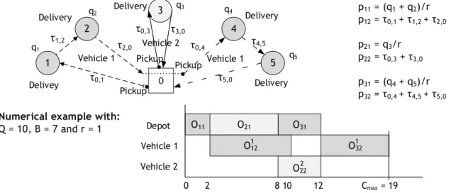
Figure 1 represents a solution of a PTSPm with two vehicles and five customers. In this solution, the customers are divided into three groups to define three jobs:
the first job (with the operations 𝑂11 and 𝑂121 ) includes customers 1 and 2;
the second job (with the operations 𝑂21 and 𝑂222 ) contains customer 3;
the third job (with the operations 𝑂31 and 𝑂321 ) includes customers 4 and 5;
The trip of vehicle 1 is composed of two transportation operations (𝑂121 and 𝑂321 ) and the trip
of vehicle 2 is composed of one transportation operation 𝑂222 . The solution presented on the Gantt chart uses the following values for the demands of the customers, 𝑞1 = 1, 𝑞2 = 1, 𝑞3 = 6, 𝑞4 = 1, 𝑞5 = 3, and the transportation times are equal to 𝜏0,1 = 𝜏2,0 = 𝜏0,4 = 𝜏4,5 = 3,
𝜏1,2 = 𝜏0,3 = 2 and 𝜏5,0 = 1. For the first job, the duration of the production operation 𝑝1 = 2 time units since the production rate 𝑟 = 1 and 𝑞1 = 𝑞2 = 1, and the duration of the transportation operation 𝑡1 = 8 time units since 𝜏0,1+ 𝜏1,2+ 𝜏2,0 = 8. The lifespan of the
product is repected: 𝑓𝑗2− 𝑓11− 𝜏2,0 = 10 − 2 − 3 = 5 ≤ 𝐵 = 7.
Let us note that τx,y in this problem denotes a transportation time between customer x and
customer y that can be precomputed by considering either the minimal distance traveled by the vehicle between customers or the minimal time necessary to travel between two customers that are equal since the speed factor for the vehicles is equal to one. The jobs have to be defined and ordered in order to minimise the makespan 𝐶𝑚𝑎𝑥, i.e., the arrival time of the last vehicle at the depot. p11 = (q1 + q2)/r p12 = τ0,1 + τ1,2 + τ2,0 p21 = q3/r p22 = τ0,3 + τ3,0 p31 = (q4 + q5)/r p32 = τ0,4 + τ4,5 + τ5,0
Numerical example with:
Q = 10, B = 7 and r = 1 1 2 3 4 5 0 q1 q2 q4 q5 τ0,1 τ2,0 τ1,2 τ0,4 τ4,5 τ3,0 τ5,0 τ0,3 Delivey Delivery Delivery Delivery Delivery Vehicle 1 Vehicle 1 Vehicle 2 Pickup Pickup Pickup O11 O31 0 2 8 10 12 Cmax = 19 O21 O12 O32 O22 Depot Vehicle 1 Vehicle 2 1 1 2 q3
Figure 1. Example of one PTSPm solution with five customers and two vehicles.
2.2 Linear formulation of the PTSPm
The combined production scheduling and vehicle routing problem is formulated as a mixed integer linear programming model based on five binary variables (𝑦𝑏𝑖, ℎ𝑏, 𝑥𝑖𝑗𝑏, 𝑧
𝑏𝑐, 𝑎𝑏𝑘) and
seven integer variables (𝑠𝑏1, 𝑠𝑏2,𝑝𝑏1, 𝑝𝑏2, 𝑝𝑏2′ , 𝑞𝑖−, 𝐶𝑚𝑎𝑥). The binary decision variables are
related to the disjunctions between operations and the integer variables are related to the starting and finishing times or duration of the operations.
Notations for the binary variables: 𝑦𝑏𝑖 = {10 if customer 𝑖 is in job 𝑏
otherwise
𝑖 ∈ 𝐸 𝑏 ∈ 𝐽 ℎ𝑏= {1 0 if job 𝑏 is composed of at least one customer
otherwise
𝑏 ∈ 𝐽 𝑥𝑖𝑗𝑏 = {1 0 if customer 𝑖 is serviced immediately before customer 𝑗 in job 𝑏
otherwise
(𝑖, 𝑗) ∈ 𝐸2
𝑏 ∈ 𝐽 𝑧𝑏𝑐 = {1
0 if job 𝑏 is scheduled before job c otherwise
(𝑏, 𝑐) ∈ 𝐽2
𝑎𝑏𝑘 = {1
0 if job 𝑏 is assigned to vehicle 𝑘 otherwise
𝑏 ∈ 𝐽 𝑘 ∈ 𝑉
Job assignment requirement: this set of constraints ensures that one customer is assigned to
one and only one job.
Vehicle capacity requirements: this constraint ensures that the customers assigned to a job can
be serviced by one vehicle considering the total amount of demands of customers.
∀𝑏 ∈ 𝐽 ∑𝑖∈𝐸𝑦𝑏𝑖. 𝑞𝑖 ≤ 𝐶 (2)
Job definition: this constraint ensures that if job 𝑏 encompasses no customer (ℎ𝑏 = 0), no
customer is assigned to the job (𝑦𝑏𝑖 = 0)
∀𝑏 ∈ 𝐽, ∀𝑖 ∈ 𝐸 𝑦𝑏𝑖 ≤ ℎ𝑏 (3)
Job duration for the production: this constraint defines the job processing time 𝑝𝑏 on the
production considering the set of customers assigned to the job. If customer 𝑖 is assigned to job 𝑏, then 𝑦𝑏𝑖 = 1 and ∑𝑖∈𝐸𝑞𝑖. 𝑟 is the sum of 𝑞𝑖 moderated with the production rate 𝑟.
∀𝑏 ∈ 𝐽 𝑝𝑏 = ∑𝑖∈𝐸𝑦𝑏𝑖. 𝑞𝑖. 𝑟 (4)
Vehicle assignment to one vehicle: this constraint ensures that if job 𝑏 is used (there are one
or several customers assigned to 𝑏), i..e., ℎ𝑏 = 1, then one variable 𝑎𝑏𝑘 is assigned to 1, i.e., one vehicle 𝑘 is assigned to job 𝑏.
∀𝑏 ∈ 𝐽 ℎ𝑏= ∑𝑘∈𝑉𝑎𝑏𝑘 (5)
Customer order in the jobs: this set of constraints ensures that each customer has a single
predecessor and a single successor
∀𝑗 ∈ 𝐸 ∑ ∑𝑖∈𝐸∪{0}𝑥𝑖𝑗𝑏 𝑖≠𝑗 𝑏∈𝐽 = 1 (6) ∀𝑖 ∈ 𝐸 ∑ ∑𝑗∈𝐸∪{0}𝑥𝑖𝑗𝑏 𝑗≠𝑖 𝑏∈𝐽 = 1 (7)
Depot definition: this constraint ensures that if job 𝑏 encompasses at least one customer
(ℎ𝑏 = 1), the sub-trip starts and ends at the depot.
∀𝑏 ∈ 𝐽 ℎ𝑏= ∑ 𝑥0𝑗𝑏
𝑗∈𝐸 (8)
∀𝑏 ∈ 𝐽 ℎ𝑏= ∑𝑖∈𝐸𝑥𝑖0𝑏 (9)
Customer assignment to a job: this constraint ensures that if a customer 𝑖 is assigned to job 𝑏
(𝑦𝑏𝑖 = 1), then customer 𝑖 has one predecessor, i. e., ∃𝑗/𝑥𝑖𝑗𝑏 = 1. Similar remarks hold for
constraint 13, considering the successor. ∀𝑖 ∈ 𝐸, ∀𝑏 ∈ 𝐽 𝑦𝑏𝑖 = ∑𝑗∈𝐸∪{0}𝑥𝑖𝑗𝑏
𝑗≠𝑖 (10)
∀𝑖 ∈ 𝐸, ∀𝑏 ∈ 𝐽 𝑦𝑏𝑖 = ∑𝑗∈𝐸∪{0}𝑥𝑗𝑖𝑏 𝑗≠𝑖
(11)
Sub-trip eliminations: these constraints are the Miller-Tucker-Zemlin (MTZ) constraints. This constraint uses 𝑞𝑗−, referred to as the total amount of products remaining in the vehicle after servicing customer 𝑗.
∀𝑏 ∈ 𝐽, ∀(𝑖, 𝑗) ∈ 𝐸2, 𝑖 ≠ 𝑗 𝑞
𝑗−− 𝑞𝑖−+ 𝑥𝑖𝑗𝑏. 𝐶 ≤ 𝐶 − 𝑞𝑗 (12)
∀𝑏 ∈ 𝐽, ∀(𝑖, 𝑗) ∈ 𝐸2, 𝑖 ≠ 𝑗 𝑞
𝑖− ≤ 𝐶 − 𝑞𝑖 (13)
Job duration for transport: this constraint defines the sub-trip duration to service all customers
assigned to job 𝑏
∀𝑏 ∈ 𝐽 𝑝𝑏2 = ∑ ∑𝑗∈𝐸∪{0}𝑥𝑖𝑗𝑏
𝑗≠𝑖
. 𝜏𝑖𝑗
𝑖∈𝐸∪{0} (14)
Job duration for transport: this constraint defines the trip duration to service all customers
assigned to job 𝑏 not considering the empty transport from the last customer to the depot.
∀𝑏 ∈ 𝐽 𝑝𝑏2′ = 𝑝
𝑏2− ∑𝑖∈𝐸𝑥𝑖0𝑏. 𝜏𝑖0 (15)
Disjunctive constraints at the production end: this constraint ensures that the production
operation of job 𝑐 and the production operation of job 𝑑 cannot be performed at the same time at the production facility.
∀(𝑏, 𝑐) ∈ 𝐽2, 𝑐 ≠ 𝑏 𝑠
𝑏1+ 𝑝𝑏1 ≤ 𝑠𝑐1+ (1 − 𝑧𝑏𝑐). 𝐻 (16)
∀(𝑏, 𝑐) ∈ 𝐽2, 𝑐 ≠ 𝑏 𝑠
If 𝑧𝑏𝑐 = 1 (job 𝑏 is scheduled before job 𝑐), constraint (18) can be rewritten as 𝑠𝑏1+ 𝑝𝑏1− 𝑠𝑐1 ≤ 0, meaning that 𝑠𝑏1+ 𝑝𝑏1 ≤ 𝑠𝑐1, ensuring that production of 𝑐 on the production facility cannot start before the end of the production operation of job 𝑏. If 𝑧𝑏𝑐 = 0, constraint (18) holds, and constraint (19) can be rewritten as 𝑠𝑐1+ 𝑝𝑐1≤ 𝑠𝑏1, meaning that job 𝑐 is processed first and job 𝑑 second for the production operations.
Disjunctive constraints for transport: this constraint ensures that the transport operations of
two jobs 𝑏 and 𝑐 are not performed at the same time by the same vehicle 𝑘. ∀(𝑏, 𝑐) ∈ 𝐽2, 𝑐 ≠ 𝑏 𝑠
𝑏2+ 𝑝𝑏2 ≤ 𝑠𝑐2+ (3 − 𝑧𝑏𝑐− 𝑎𝑏𝑘 − 𝑎𝑐𝑘). 𝐻 (18)
∀(𝑏, 𝑐) ∈ 𝐽2, 𝑐 ≠ 𝑏 𝑠
𝑐2+ 𝑝𝑐2 ≤ 𝑠𝑏2+ (2 − 𝑧𝑏𝑐 + 𝑎𝑏𝑘+ 𝑎𝑐𝑘). 𝐻 (19)
If 𝑎𝑏𝑘 = 𝑎𝑐𝑘 = 1, this means that the two transport operations are assigned to the same vehicle
𝑘 and the constraints can be rewritten as: 𝑠𝑏2+ 𝑝𝑏2≤ 𝑠𝑐2+ (1 − 𝑧𝑏𝑐). 𝐻 (20) and 𝑠𝑐2+ 𝑝𝑐2≤ 𝑠𝑏2+ 𝑧𝑏𝑐. 𝐻 (21). If either 𝑎𝑏𝑘 or 𝑎𝑐𝑘 are not assigned to 1, the two constraints hold, regardless of the value of 𝑧𝑏𝑐.
Precedence constraints per operation: this constraint ensures that the transport operations of
one job are performed according to the production-operation sequence first, followed by the transport-operation sequence.
Lifespan products: this constraint ensures that the lifespan of the products are addressed. The
product lifespan defines a maximal delay between the delivery of the last customer of a sub-trip of a job b, i.e., 𝑠𝑏2+ 𝑝𝑏2′ , and the finishing time of the production referred to as 𝑠
𝑏1+ 𝑝𝑏1:
the difference is upper bounded by 𝐵.
∀𝑏 ∈ 𝐽 𝑠𝑏2+ 𝑝𝑏2′ ≤ 𝑠𝑏1+ 𝑝𝑏1+ 𝐵 (21)
Makespan. When minimising the makespan, the following constraints should be added to define new integer variables. This constraint ensures that 𝐶𝑚𝑎𝑥 = 𝑚𝑎𝑥𝑏∈𝐽(𝑑𝑏2+ 𝑝𝑏2)
∀𝑏 ∈ 𝐽 𝑠𝑏2+ 𝑝𝑏2 ≤ 𝐶𝑚𝑎𝑥 (22)
2.3 Modelling
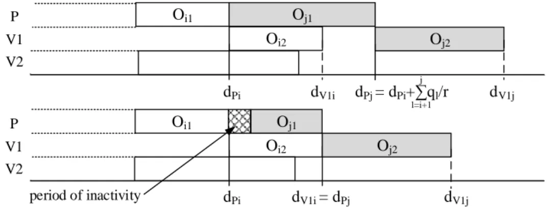
In the PTSPm, a sub-trip is fully defined by an ordered sequence of operations: (1) starting at the depot with a pickup operation; (2) defining an ordered sequence of delivery operations; and (3) finishing at the depot. The loading of the vehicle can be represented as a decreasing function (see Fig. 2) during each sub-trip.
Figure 2 gives some details of the solution presented in Fig. 1. Figure 2 represents both the vehicle load (on the top) and the proper coordination between production and transportation over time, with an explicit modelling of pickup and delivery operations (at the bottom).
Table 2. Example of solution for the two-vehicle PTSPm.
𝑂11 𝑂12 1 𝑂21 𝑂22 2 𝑂31 𝑂32 1 0 1 2 0 0 3 0 0 4 5 0 Starting time 0 2 8 Time Windows ]-∞;9] ]-∞;15] ]-∞;19] Departure time 2 5 7 8 10 12 15 18 Arrival time 5 7 10 10 12 15 18 19
Time constraints on sub-trips
Time dependency only exists between successive trips of the same trip since all sub-trips of one trip are assigned to the same vehicle. Concerning the trip of vehicle 1 in Fig. 2, the previous remark implies that 𝑠32≥ 𝑓12. Moreover, the earliest starting time of 𝑂31 depends on the starting time 𝑂21, 𝑠31 ≥ 𝑠21+ 𝑝21. For the trip of vehicle 2, the earliest starting time of the transportation operation 𝑂222 does not depend on the finishing time of 𝑂121 (operations in the diagonal rectangle in Fig. 2). Vehicle 2 can potentially start the transportation operation 𝑂222 before the transportation operation 𝑂121 , as depicted in Fig. 2 and Table 2. Assignment of
vehicles to sub-trips is a challenging problem that should be solved avoiding extra waiting time on the Gantt chart.
s12 End of trip 1 Time Vehicle loading 0 O12
Node 1 Node 2 Node 3 Node 4 Node 5
]-∞,y] P D P D P D D -y -x -z τ0,1 τ1,2 τ0,3 O11 0 O31 s21 s11 s31 0 0 0 O21 p31 τ3,0 * p21 p31 0 0 0 Prod. Trip 1 τ2,0 τ0,4 τ4,5 τ5,0 End of trip 2 0 Trip 2 S 0
No time dependency between the finishing time of
and the starting time of
0 p11 p11 D p21 f12 s32 f32 s22 f22 1 O222 O32 1 O121 O222 ]-∞,x] ]-∞,z]
Figure 2. Example of a two-vehicle workload.
Conjunctive and disjunctive arcs to link production and transportation with maximal time lags The delivery nodes where products are unloaded have a time window constraint that defines the maximal arrival time acceptable for the customer, which is correlated to the product perishability. The time windows are related to the earliest starting time of the production on the facility. They are modelled by maximal time lags that are defined using a negative arc between one delivery node and the production node in this special case.
As shown in Fig. 2, the time window ] − ∞; 𝑦] on node 2, which corresponds to a delivery node, means that the maximal duration between 𝑠11 and the arrival time at node 2 must not exceed 𝑦 units of time. Similarly, node 3 must be served within a delay of 𝑥 units of time after 𝑠21. One positive arc gives the minimal delay between the earliest starting time of two operations. For example, τ1,2 models a minimal duration required between departure time at node 1 and arrival time at node 2. Normally, these so-called conjunctive arcs are valuated with the shortest path value between two nodes modelling transport, and with the duration of production between two production nodes. Disjunctive arcs are required to define the order of sub-trips in a trip. This type of time windows arises: (1) in routing problems including but not limited to the Dial-A-Ride Problem where both maximal route duration and maximal customer riding time must be taken into account; and (2) in scheduling problems.
In the Gantt chart in Fig. 1, the first job provides products for customers 1 and 2 for a production duration of 𝑝11= 2 time units, the earliest starting time of 𝑂11 is equal to 0 and vehicle 1 is available at time 0. Therefore, on node 1 (Fig. 2), the time window is defined by ] − ∞; 2 + 𝛿1] and ] − ∞; 2 + 𝛿2] for node 2, where 𝛿𝑖 is the lifespan of products for
customer 𝑖. The earliest starting time of a transportation operation is the maximal value between the finishing time of the previous transportation operation assigned to the same vehicle and the finishing time of the production operation. Similar considerations make it possible to define the earliest starting time 𝑂222 at time 8 with a time window ] − ∞; 8 + 𝛿
3] for nodes 3. Because the
problem being considered is a single product PTSPm, the lifespan is equal for all nodes, i.e., 𝛿𝑖 = 𝐵, ∀𝑖, implying that all time windows of all delivery nodes of the same sub-trip are
identical and equal to ] − ∞; 𝑥 + 𝐵], where 𝑥 is the duration of the production linked to the transport.
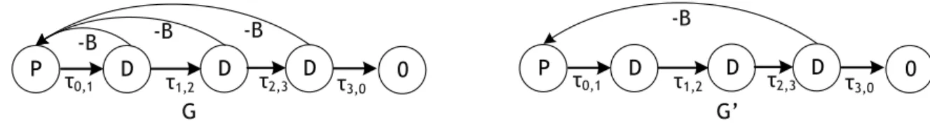
Figure 3. Sub-trip with maximal time lag simplification.
The earliest arrival time of a vehicle increases within a sub-trip. Therefore, if an earliest arrival time exists for the last delivery operation of the sub-trip that meets the time window constraints, all previously scheduled operations with time window constraints will hold. In Fig. 3, sub-trip 𝐺 with three delivery nodes takes the three maximal time lags modelling the product lifespan explicitly into account. For PTSPm with a single product, which consequently defines the same lifespan for all customers, a new graph 𝐺′ can be used to model only the time window of the last delivery operation of each sub-trip.
The feature that differentiates this problem from previous ones is the combination of the scheduling decisions with the limited product lifespan and the vehicle routing decisions. These interdependent decisions lead to the possibility that the product may expire before it reaches a customer if an unprofitable scheduling solution is chosen. The objective consists in solving the scheduling and routing problem by minimising the makespan to comply with the classical objective function introduced by Geismar et al. (2008) and providing a semi-active solution, i.e., a left-shifted solution.
3 A PTSPm resolution based on a GRASP ELS
This proposal is based on a GRASP×ELS, which introduces a new splitting algorithm for the assignment and the routing problem, and a new resolution of the scheduling problem using an approach based on a disjunctive graph. The disjunctive graph is specially designed to efficiently take the perishability constraint into account using maximal time lags.
3.1 Key features for a PTSPm resolution
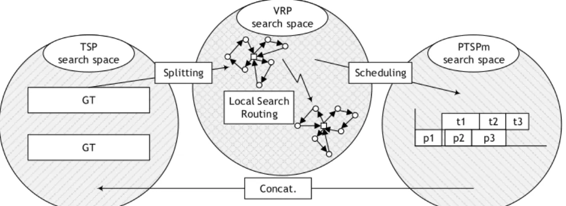
The key point for the PTSPm resolution is to alternate between solutions encoded by giant trips (TSP - Traveling Salesman Problem - permutation list on the 𝑛 customers), set of trips (VRP - Vehicle Routing Problem - on the 𝑛 customers) that comply with the ordered set of customers defined by the giant trip, and a flow shop resolution by considering jobs linked to the trips (PTSPm on the 𝑛 customers). The approach is a combination of three search space representations that favour partial enumeration of the whole search space (Fig. 4).
The iterative search space exploration takes advantage, first, of the indirect representation of solutions by using a giant trip. Second, a set of feasible sub-trips minimising the total transportation time is computed using a split-based approach on the sequence of customers that has been defined by the giant trip. Note that the specific local search for node routing can be applied to obtain a high-quality local routing solution.
The resolution framwork is expressed by the following key features:
a local search for routing with 2-Opt or swap within a sub-trip, and 2-Opt or swap between two sub-trips, based on classical VRP neighbourhoods;
a splitting procedure for proper coordination between production and transportation;
a scheduling procedure based on a disjunctive graph with the sub-trips made by the splitting procedure;
a concatenation procedure to obtain a new giant trip.
P -B D D -B τ0,1 τ1,2 τ2,3 D τ3,0 0 -B P τ D D 0,1 τ1,2 τ2,3 D τ3,0 0 -B G G’
TSP search space PTSPm search space VRP search space GT GT Splitting Local Search Routing Scheduling Concat. t2 t1 p1 p2 p3 t3
Figure 4. The three search spaces to build a PTSPm solution.
The GRASP×ELS approach is very different from Geismar et al.’s proposal and differs in both scope and the resolution scheme that are summarised in Table 3.
Table 3. GRASP×ELS approach vs. Geismar et al.’s approach
(Geismar et
al., 2008) GRASP×ELS
Scope PTSP PTSP + PTSPm
Resolution scheme
Scheduling Gilmore-Gomory Disjunctive graph
Routing classical VRP Split of the Split with production and transport consideration Local search
for scheduling /
Based on the proposal of Laarhoven et al. (1992) and
Grabowski et al. (1986) Local search
for routing 2-Opt moves
Inter/extra trips 2-Opt and swap moves
Solution
representation Chromosome Giant trip
3.2 The GRASP×ELS Principle
GRASP×ELS is a hybridisation (Prins, 2009) of a GRASP (Greedy Randomised Adaptive Search Procedure) (Feo and Resende, 1995), with an ELS (Evolutionary Local Search) (Wolf and Merz, 2007; Prins, 2004) that takes advantage of both methods. The multi-start approach of the GRASP, which provides 𝑛𝑝 initial solutions, is based on a greedy randomised heuristic, and solutions are then improved by a local search procedure. The second metaheuristic can be expressed as an extension of the ILS (Iterated Local Search) (Lourenço et al., 2003), referred to as ELS and proposed by Wolf and Merz (2007). The solution space investigation is achieved by the GRASP that favours diversity, and the intensification phase is devoted to the ELS via a proper local search investigation into the local search space. In addition, to combine GRASP with ELS, another important feature is the alternation between solution spaces as stressed by Prins (2004) and Prins et al. (2014). Converting a PTSPm solution into a giant trip is achieved by a concatenation procedure, and the operation converting a giant trip into a VRP solution is achieved by a dedicated splitting procedure (Split).
Algorithm 1 is composed of a loop from line 13 to 36, which iterates on a new starting solution for the GRASP. For each initial solution, the procedure
Generation_of_initial_solution(), using a greedy heuristic creates a new initial solution submitted to the Split procedure (line 16) to obtain a routing solution that is improved (line 17) by the local search procedure Local_Search_on_Routing(S, nl). Secondly, the
Scheduling() procedure computes a solution (line 18). If the cost of the solution 𝑆, 𝑓(𝑆) is
better than the cost of the best PTSPm solution found, 𝑆*, 𝑓* (line 20), 𝑆 becomes the new best solution. The while loop from lines 23 to 35 is the ELS and encompasses the loop (lines 25 to
32) for neighbourhood generations. According to the common Split approach, the mutation operator (line 26) is defined on the giant trip T and not on the solution.
The random heuristics, referred to as Generation_of_initial_solution(), generates initial solutions. This method uses two heuristics to build the initial solution.
The first one, with a probability of 0.9 is based on a greedy randomised heuristic based on a path-scanning-like approach. The first heuristic builds sub-trips one-by-one, starting from the depot, and extends each sub-trip customer-by-customer using two criteria:
the extension step at node 𝑖 considers that the sub-trip moves to the nearest customer not yet served. If vehicle load ≥ 𝑄, the next customer to be served is selected to minimise the distance to the depot;
the next customer to be served is the customer that minimises the transportation time. The second heuristic with a probability of 0.1 classifies the customers by decreasing transportation time.
Algorithm 1. GRASP ELS for the PTSPm
1. procedure GRASP ELS 2. global parameters
3. np: number of GRASP iterations (initial solutions) 4. ne: maximal number of iterations per ELS
5. nr: maximal number of iterations without improvement per ELS 6. nd: number of diversifications (mutations)
7. nl: number of local searches on the routing 8. ng: number of local searches on the scheduling 9. output parameters
10. S*: best PTSPm solution found 11. begin
12. f* := ; O := Ø
13. for p := 1 to np do // GRASP loop 14. S := call Generation_of_initial_solution () 15. T := call Concat (S) 16. S := call Split (T) 17. S := call Local_Search_on_Routing (S, nl) 18. S := call Scheduling (S) 29. T := call Concat (S)
20. if (f(S) < f*) then f* := f(S); S* := S; // f: the cost of a solution 21. endif
22. i, r := 0
23. while (i < ne) and (r < nr) do // ELS loop
24. i := i + 1; f” :=
25. for j := 1 to nd do // mutation loop 26. T’ := call Mutation (T) 27. S’ := call Split (T’) 28. S’ := call Local_Search_on_Routing (S’, nl) 29. S’ := call Scheduling (S’) 30. T’ := call Concat (S’) 31. if (f(S’) < f”) then f” := f(S’); T” := T’; S” := S’; endif 32. endfor
33. if (f” < f*) then S*:= S”; endif // if a new best solution update S* 34. T := T”; // best ELS solution becomes the new initial solution 35. endwhile
36. endfor 37. end
The local search on the routing (Local_Search_on_Routing()) is achieved using several classical VRP neighbourhood moves to improve the initial solution, namely 2-Opt within a sub-trip and insertion within a sub-sub-trip. At each iteration, the first improved move is executed but requires verification of the sub-trip feasibility by considering the capacity of the vehicles and the lifespan. All solutions are converted into a giant trip by random concatenation of their sub-trips and then evaluated by the Split procedure. The key point for the efficiency of GRASP×ELS is to alternate between solutions encoded as giant trips and PTSPm solutions.
3.3 Split procedure
Giant trips are evaluated via the Split procedure that minimises the total trip duration subject to the vehicle capacity, as reported by Beasley (1983) and Prins et al. (2014). Split is a key procedure used to convert a giant trip into a VRP solution (with respect to the sequence) and it is based on the classical Split procedure adjusted to address the specific PTSPm constraints. The algorithm provides an efficient solution by building an auxiliary graph 𝐺 = (𝑋, 𝐴), where X represents n + 1 nodes numbered from 0 to n. Node 0 is a dummy node, while the nodes 1 … n correspond to the sequence of the giant trip 𝐺𝑇 = (𝜎1, … , 𝜎𝑛). An arc (𝑖, 𝑗) belongs to A
if a sub-trip serving customers 𝜎𝑖+1 to σj (inclusive) is both weight-feasible and
lifespan-feasible. An initial label is set at node 0 and the labels are propagated from node to node in G using arcs. The best label at node 𝑛 is kept as the best solution.
The routing problem has a resource constraint since there is a limited number of available vehicles, each vehicle defining one specific machine to be scheduled. The Split procedure for the PTSPm is an extension of the split introduced for the HVRP (Heterogeneous Vehicle Routing Problem) by Duhamel et al. (2012) because there is the earliest finishing time of the production to take into account as well as the earliest finishing time of vehicles for the previous sub-trip. Computation of the resource-constrained shortest path in the graph is typically achieved by a label-correcting algorithm. According to Desrocher (1988), several labels per node have to be handled and the key point consists in defining the label structure with the cost and the resource availability. The generic Split procedure of Duhamel et al. (2012) is based on three key points:
a label description based on the resource availability;
a dominance rule between labels to improve the running time by keeping only promising labels on the node;
a propagation rule to define a label from node 𝑖 to node 𝑗 depending on the customer sequence (σi+1, … , σj).
Let 𝐿𝑝𝑖 = (𝑑𝑃𝑖, 𝑑𝑉1𝑖, … , 𝑑𝑉𝑁𝑖) be the 𝑝𝑡ℎ label assigned to node 𝑖 when the number of
vehicles 𝑉 = 𝑁, where Lip(𝑗) is the earliest finishing time of vehicle 𝑗 for 𝑗 = 2. . 𝑁 + 1 and
Lip(1) is the earliest finishing time of the production. This corresponds to a feasible split of the initial customers (𝜎1, … , 𝜎𝑖) into sub-trips, where dPi is the earliest production finishing time
and dVki is the transportation finishing time for the vehicle 𝑉𝑘. The initial label at node 0 is defined as 𝐿10 = (0, 0, … , 0). It corresponds to the empty solution where the finishing time is
equal to 0. Given the arc (𝑖, 𝑗) ∈ 𝐴 and if this arc is put on vehicle 𝑉𝑘, label Lpi generates label
𝐿𝑗𝑞 = (𝑑𝑃𝑗, 𝑑𝑉1𝑗, … , 𝑑𝑉𝑁𝑗) using the following propagation rule:
𝑑𝑃𝑗 = 𝑚𝑎𝑥( 𝑑𝑃𝑖+ ∑ 𝑝𝜎𝑙 𝑗 𝑙=𝑖+1 ; 𝑑𝑉𝑘𝑖 ) = 𝑚𝑎𝑥( 𝑑𝑃𝑖+ ∑ 𝑞𝜎𝑙 𝑟 𝑗 𝑙=𝑖+1 ; 𝑑𝑉𝑘𝑖 ) 𝑑𝑉𝑘𝑗 = 𝑑𝑃𝑗 + 𝜏0,𝜎𝑖+1 + ∑𝑗−1𝑙=𝑖+1𝜏𝜎𝑙,𝜎𝑙+1+ 𝜏𝜎𝑗,0.
The max operator, which appears in the propagation rule, is explained in Fig. 5. In the first case, 𝑂𝑗1 has a duration (𝑝𝑗1) greater than the duration between the end of the production operation 𝑂𝑖1 at time 𝑑𝑃𝑖 and the end of the previous sub-trip assigned to vehicle 𝑉1 (𝑑𝑉1𝑖). The finishing time of 𝑂𝑖1 therefore corresponds to the starting time of 𝑂𝑗1 and, consequently, 𝑑𝑃𝑗 = 𝑑𝑃𝑖+ ∑
𝑞𝜎𝑙 𝑟 𝑗
𝑙=𝑖+1 . In the other case, if 𝑂𝑗1 has a duration (𝑝𝑗1) lower than
the duration between the end of the production operation 𝑂𝑖1 at time 𝑑𝑃𝑖 and the end of the
previous sub-trip assigned to vehicle 𝑉1 (𝑑𝑉1𝑖), then to be compliant with the no-wait
constraint, the constraint 𝑑𝑃𝑗 = 𝑑𝑉1𝑖 must hold and the production planning will encompass a period of inactivity.
Oi1 dPi dV1i Oi2 Oj1 Oj2 Oi1 dPi dV1i = dPj dV1j Oi2 Oj1 Oj2 dPj = dPi+∑ql/r dV1j l=i+1 j period of inactivity V2 V1 P V2 V1 P
Figure 5. The two cases of label propagation in the Split procedure.
Since a large number of labels may be generated, dominance criterion is used to improve the running time, keeping only non-dominated labels on the node thanks to the following dominance propriety.
Dominance property
Label L = (𝑑𝑃, 𝑑𝑉1, … , 𝑑𝑉𝑁) dominates label P = (𝑑𝑃, 𝑑𝑉1, … , 𝑑𝑉𝑁) when the two labels are
sorted and is therefore equal to (𝑑𝜎1𝑝, … , 𝑑𝜎𝑁+1𝑝 ) and (𝑑𝜎1𝑞, … , 𝑑𝜎𝑁+1𝑞 ), respectively, and all of the following conditions hold:
∃𝑖∗ ∈ {1, … , 𝑁 + 1}, d
σ𝑖𝑝∗ < dσ𝑖𝑞∗; ∀𝑗 ∈ {1, … , 𝑁 + 1}, dσ𝑗𝑝 ≤ dσ𝑗𝑞∗.
The dominance rule limits the number of labels stored at each node but several authors, including (Duhamel et al., 2012), have reported that a large number of labels could still be generated. Another time-saving approach consists in limiting the maximal number 𝑁𝑚𝑎𝑥 of labels generated during the split process and the maximal number 𝑁𝐵𝑚𝑎𝑥 of labels stored at each node. This can reduce the CPU time, but discarding some labels may cause the algorithm to miss the optimal split. Such an approach offers a compromise between split quality and the number of labels kept on nodes and provides time-efficient sub-optimal split solutions.
The Split procedure is detailed in Algorithm 2 and uses low-level procedures to handle the label on the graph:
Propagation_label_to_vehicle(L,v,𝑖) propagates the label 𝐿 using the vehicle v at node 𝑖 and returns a new label;
CheckDomination(L, i, Ni) performs the dominance check between the label 𝐿
and all labels stored at node 𝑖, 𝑁𝑖. It returns 0 if 𝐿 is dominated by at least one label from 𝑖. Thus, 𝐿 must not be saved. It returns 1 if 𝐿 dominates at least one label from 𝑖. It returns 2 otherwise;
InsertLabel(L, i, CD, Ni, NBmax)attempts to add the label 𝐿 at node 𝑖 if 𝐶𝐷 ∈
{1,2} and by considering that the number of labels 𝑁𝑖 must not exceed the maximal
number 𝑁𝐵𝑚𝑎𝑥. If 𝐶𝐷=1, all labels from i dominated by 𝐿 are deleted. The list of labels is
ordered by decreasing cost;
Extract_trip() checks the shortest path into the graph for the last node to the first node, and returns the set of trips.
The Split algorithm (Algorithm 2) is composed of two parts: the initialisation part where local variables are initialised (lines 14-15) and a for loop from lines 16 to 52, which iterates for the ordered set of customers defined by the giant trip T. The while loop from lines 19 to 51 iterates and makes it possible to evaluate the partial sequence (𝜎𝑖+1, … , 𝜎𝑗). If 𝑖 = 𝑗, a new sub-trip is created and the initial sub-trip costs are assigned (lines 22- 23) and are updated in lines 25-26.
The condition line 28 makes it possible to determine if the constraints hold and the loop is stopped early thanks to the condition on the Boolean condition (stop=true). Because a set of labels is saved at each node, the for loop of line 29 iterates over all labels of node i and addresses the label 𝐿𝑃𝑖. Algorithm 2. Split 1. procedure Split 2. input parameters 3. T: giant tour 4. output parameters 5. S: VRP-PTSPm solution 6. global parameter
7. Q : maximal vehicle weight capacity 1. B : lifespan of the product
8. qi : total items ordered by customer i
9. 𝜏ij : cost from customer i to j
10. n : number of customers 11. N : number of vehicles
12. NBmax : maximal number of labels in each node
13. begin 14. L01:=(0,0,…,0), S := 15. for i := 1 to n do NBi := 0 endfor 16. for j := 0 to n do 17. j := i 18. stop := false
19. while (j < n and stop=false)
20. customer := Tj
21. if (j = i) then
22. production_cost := dcustomer/r
23. transport_cost := cdepot,customer + ccustomer,depot
24. else
25. production_cost += dcustomer/r
26. transport_cost += ccustomer-1,customer +ccustomer,depot –ccustomer-1,depot
27. endif
28. if ((production_cost*r < Q) and (transport_cost -ccustomer,depot ≤ B)) then
29. for p := 1 to NBi do
30. if (dPi-1 = 0) then
31. insertion of the label in first position with the first vehicle 32. else 33. v:=0 34. do 35. v:=v+1 36. L:=Propagation_label_to_vehicle (Lip,v,i) 38. if (NBi=0)
39. insertion of L in first position 40. else
41. CD:=CheckDomination(L, j, Nj)
42. call InsertLabel(L, j, CD, Nj, NBmax)
43. endif 44. while (v < N) 45. endif 46. endfor 47. else 48. stop := true 49. endif 50. j := j + 1 51. endwhile 52. endfor
53. S := call Extract_trips () //save the best solution 54. endif
55. end
A full example is given in detail on the Web page:
3.4 Scheduling procedure
After the splitting procedure, each job is fully defined by an ordered sequence of customer demands that are assigned to a specific vehicle. The previous sections refer to a problem that can be defined as a two-stage hybrid flow shop with one machine at the first stage and 𝑁 machines at the second stage. At the first stage, the term ‘machine’ is a general term that refers to the production (production machine) and to the transportation for the second stage (also referred to as transportation machine).
A job simultaneously models the production (the first operation on the production machine) and a sub-trip (the transportation operation on one transportation machine among the 𝑁 machines available).
The problem is modelled as a disjunctive graph model first defined by Roy et al. (1964) using a directed graph G = (V, A, EP, ET), where V represents the set of nodes that contains one element for each operation 𝑂𝑖, a source node 0 connected to the first operation of each job, and
a sink node ∗ linked to the last operation of each job (Fig. 6). The set A represents the set of conjunctive arcs, EP the set of pairs of disjunctive arcs between the production nodes, and ET
the set of pairs of disjunctive arcs between the transportation nodes.
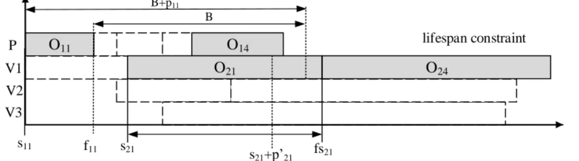
With the specific graph characteristic, the classical disjunctive graph can be adapted using maximal time lags between the starting time of the production operation 𝑂𝑖1 and the starting time of the transportation operation 𝑂𝑖2, which is consistent with the perishability constraints. The value of the maximal time lag defines the larger gap between the starting time of 𝑂𝑖1 and the starting time of 𝑂𝑖2, and is defined by −(𝐵 + 𝑝𝑖1− 𝑝′𝑖2).
Conjunctive arcs are used to connect each pair of consecutive operations of the same job. Each pair of disjunctive arcs on the production connects operation 𝑂𝑖1 to 𝑂𝑗1 (belonging to
different jobs), and has a duration 𝑝𝑖1. Each pair of disjunctive arcs on the transportation
connects two operations 𝑂𝑖2, 𝑂𝑗2 in this order belonging to different jobs that are to be processed on the same transportation machine (vehicle), and has a duration 𝑝𝑖2 (Fig. 6). A feasible solution corresponds to an acyclic graph, and an evaluation procedure can be defined using a Bellman-like longest path algorithm to obtain the earliest starting time of each operation, including the makespan 𝐶𝑚𝑎𝑥. P V1 P V2 P V1 P V2 P V3 0 * p21 p22 p23 p24 p25 p11 p21 p31 p41 p51 VB = [2,1,3,5,4] p21 p11 p31 p51 p22 p21 Disjonctive arc on the production Disjonctive arc on the transportation
First stage Second stage
-(B+p11-p’21)
-(B+p21-p’22)
-(B+p31-p’23)
-(B+p41-p’24)
-(B+p51-p’25)
Figure 6. Example of the scheduling procedure with five sub-trips and V=3.
In Fig. 6, there are two disjunctive arcs on the transportation due to jobs using the same vehicle. For vehicle 1 assigned to jobs 1 and 4, the value on the disjunctive arc is equal to p21.
of operations with the lifespan constraint. The Bierwirth vector used in the scheduling procedure gives an order on the job using the sub-trips created by the splitting procedure. An efficient local search algorithm can be defined considering the critical path including the neighbourhood of Laarhoven et al. (1992) and Grabowski et al. (1986) with the introduction of blocks. lifespan constraint O11 O14 O24 V2 V1 P V3 O21 B B+p11 s21 fs21 s21+p’21 s11 f11
Figure 7. Representation of the constraint due to the disjunctive arcs of the transportation. The neighbourhood of Laarhoven consists of swapping two consecutive operations assigned to the same machine along the critical path, leading to a modification of the machine disjunction. Due to the indirect representation of solutions, the operation swap is achieved in the Bierwirth vector by switching the two job numbers of the two operations in the disjunctive graph. The permutation of operations based on the block definition and located at the critical path is included in a depth first search local search investigates the move from the end of the critical path to the dummy node. If one permutation leads to a lower cost solution, the critical path exploration is restarted to the end of the graph. Note that due to computation time considerations, a maximal number of iterations ns is reached. A full example is given in detail on the Web page.
3.5 Hash function for PTSPm
To avoid premature convergence of the global algorithm and to stimulate the investigation of the part of the search space not previously investigated, it is necessary to use an efficient clone detection system. Previous research into scheduling/routing problems based on indirect representation approaches has proved that efficient clone detection must be defined considering the indirect representation or the solution. For the giant trip 𝐺𝑇, the related hash function 𝐻(𝑡) is defined as follows: 𝐻(𝑡) = ∑𝑛𝑖=1𝐺𝑇[𝑖] × 𝑖 𝑚𝑜𝑑 𝐾. 𝐺𝑇[𝑖] is the 𝑖𝑡ℎ customer in the giant trip and 𝐾 is a constant. The value of 𝐾 impacts the size of the map and the probability of collision (consequently, 𝐾 must be as large as possible considering the memory available).
3.6 Lower bound on the makespan
Three PTSP lower bounds were introduced by Geismar et al. (2008), leading to a poor evaluation with multiple vehicles. Considering sub-trips with only one customer associated with immediately available vehicles, 𝑁 ≥ 𝑛, a lower bound can be defined using Jackson’s algorithm (1955) that considers the one-machine scheduling problem with tails. To obtain the lower bound, the proposal is to extend Jackson’s earliest due date rule. The lower bound based on the Jackson rule creates an optimal schedule that minimises the maximal lateness by ordering the jobs by non-decreasing due dates because the release dates are equal to 0.
Line 18 in Algorithm 3 makes it possible to define the sum of the processing times of previously scheduled jobs. At line 19, the release date of the job is updated as the maximum between the current release date and the sum of the processing time plus the due date of the job. These two lines do not appear in Jackson’s original algorithm; they have been added to the algorithm in order to match the lower bound of the PTSPm.
Algorithm 3: A Jackson rule-based lower bound
1. procedure A lower bound based on the Jackson Rule
2. input parameters
3. J: set of job/sub-trip 4. global parameter
5. rj : release date of the job/sub-trip j 6. pj : processing time of the job/sub-trip j
7. q : sum of the processing time already scheduled 8. dj : due date of the job/sub-trip j
9. n : number of customers/sub-trip 10. output parameters
11. Cmax : lower bound 12. begin
13. L := {1, …, n}, q := 0 14. if (J ≠ ) then 15. while (L ≠ ) do
16. u := minj{rj}, j in L
17. choose i in L such as ri = u and di maximal 18. q := q + pi
19. for all k in L do rk:= max{rk, q + di}, Cmax := rk 20. L := L\{i}
21. endwhile 22. endif 23. end
To apply Algorithm 3 on the PTSPm, a parallel should be drawn between the processing time and the production time of the PTSPm, as well as between the due date and the PTSPm transportation time. The lower bound is then given by Cmax at the end of the algorithm.
4 Computational evaluation for the PTSP
The benchmark introduced by Geismar et al. (2008) is composed of three small-scale instances with 40 customers and three medium-scale instances with 50 customers, and customers’ demands are uniformly distributed between 100 and 300. The locations of the customers in the three instances with 40 or 50 customers are randomly generated in the square of 200, 300 and 400 side lengths, which denotes 12 sets of parameters (𝑆𝑃 is detailed in Table 5a). As a consequence, there are six datasets (𝐷𝑆 is is detailed in Table 5b). For each instance, the value of three parameters is set: 𝑟 ∈ {1,2,3} is the production rate; 𝑄 ∈ {300,600} is the truck capacity; and 𝐵 ∈ {300,600} is the product lifespan. We therefore have 72 resulting instances in the benchmark. Note that the distance is the transportation time between customers by considering the Euclidean distance and a vehicle speed of 1 unit of distance per unit of time.
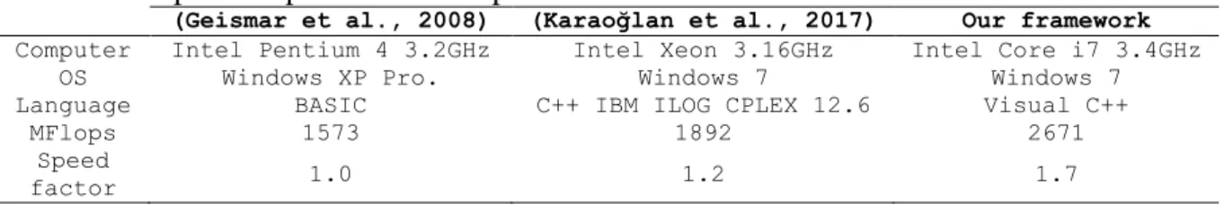
Table 4 proposes speed factors that are used in the following comparative tables to ensure a fair comparative study and that were established by previous research articles including Dongarra, (2014), and on http://www.roylongbottom.org.uk/linpackresults.htm. Since the MIPS performance is not the only influence on the CPU time, Table 4 also provides the information available about the computer, the operating system and the language.
Table 4. Comparative performance of processors.
(Geismar et al., 2008) (Karaoğlan et al., 2017) Our framework
Computer Intel Pentium 4 3.2GHz Intel Xeon 3.16GHz Intel Core i7 3.4GHz
OS Windows XP Pro. Windows 7 Windows 7
Language BASIC C++ IBM ILOG CPLEX 12.6 Visual C++
MFlops 1573 1892 2671
Speed
Five replications (𝑟𝑒𝑝) are processed for each instance and Tables 6, 7 and 8 give the average of the best solutions found over the five replications with the average CPU time required for each run. The parameters used in the GRASP×ELS are given below. They remain unchanged for all instances and were obtained after preliminary experiments:
np Number of GRASP/ELS/ neighbourhood iterations 150/30/15
lr Number of local searches on the routing/scheduling 40/500
NBmax Maximal number of labels per node 5
The following notations are used in the tables below:
C Number of customers
S Size of the square for the customer’s location
Avg An average value
%Gap N/A
Percentage gap Data not available
Nb. Opt Number of instances where the solution has the same value as the lower bound. In this case, the solution obtained is an optimal solution of the PTSPm.
𝐿𝐵𝑖𝑘 Lower bound of the problem with k ∈ SP and i ∈ DS
ℎ𝑖,𝑗𝑘 Best solution found for an instance with (𝑖; 𝑗; 𝑘) ∈ (𝐷𝑆; 𝑆𝑃; ⟦1, 𝑟𝑒𝑝⟧) 𝑡𝑡𝑖,𝑗𝑘 Total CPU time in seconds coupled with ℎ
𝑖,𝑗 𝑘 𝑡𝑖,𝑗𝑘 CPU time in seconds to get ℎ𝑖,𝑗𝑘
𝐿𝐵∗𝑘 = avg 𝑖𝜖𝐷𝑆𝐿𝐵𝑖
𝑘 Average lower bound for one k ∈ SP, over all 𝑖 ∈ 𝐷𝑆 ℎ∗,∗𝑘 = avg
𝑖𝜖𝐷𝑆,𝑗=⟦1,𝑟𝑒𝑝⟧ℎ𝑖,𝑗
𝑘 Average best solution found for one k ∈ SP, over all (𝑖; 𝑗)/(𝑖 ∈ 𝐷𝑆; 𝑗 = ⟦1, 𝑟𝑒𝑝⟧)
𝑡𝑡∗,∗𝑘 = avg
𝑖𝜖𝐷𝑆,𝑗=⟦1,𝑟𝑒𝑝⟧𝑡𝑡𝑖,𝑗
𝑘 Average total CPU time for one k ∈ SP, over all (𝑖; 𝑗)/(𝑖 ∈ 𝐷𝑆; 𝑗 = ⟦1, 𝑟𝑒𝑝⟧) 𝑡∗,∗𝑘 = avg
𝑖𝜖𝐷𝑆,𝑗=⟦1,𝑟𝑒𝑝⟧𝑡𝑖,𝑗
𝑘 Average CPU time for one k ∈ SP, over all (𝑖; 𝑗)/(𝑖 ∈ 𝐷𝑆; 𝑗 = ⟦1, 𝑟𝑒𝑝⟧) 𝐿𝐵∗∗ = avg
𝑘𝜖𝑆𝑃,𝑖𝜖𝐷𝑆𝐿𝐵𝑖
𝑘 Average lower bound over all (𝑖; 𝑘)/(𝑖 ∈ 𝐷𝑆; 𝑘 ∈ 𝑆𝑃) ℎ∗,∗∗ = avg
𝑘𝜖𝑆𝑃,𝑖𝜖𝐷𝑆,𝑗=⟦1,𝑟𝑒𝑝⟧ℎ𝑖,𝑗
𝑘 Average best solution found over all (𝑖; 𝑗; 𝑘)/(𝑖 ∈ 𝐷𝑆; 𝑗 = ⟦1, 𝑟𝑒𝑝⟧; 𝑘 ∈ 𝑆𝑃)
𝑡𝑡∗,∗∗ = avg
𝑘𝜖𝑆𝑃,𝑖𝜖𝐷𝑆,𝑗=⟦1,𝑟𝑒𝑝⟧𝑡𝑡𝑖,𝑗
𝑘 Average total CPU time over all (𝑖; 𝑗; 𝑘)/(𝑖 ∈ 𝐷𝑆; 𝑗 = ⟦1, 𝑟𝑒𝑝⟧; 𝑘 ∈ 𝑆𝑃)
𝑡∗,∗∗ = avg
𝑘𝜖𝑆𝑃,𝑖𝜖𝐷𝑆,𝑗=⟦1,𝑟𝑒𝑝⟧𝑡𝑖,𝑗
𝑘 Average CPU time for all (𝑖; 𝑗; 𝑘)/(𝑖 ∈ 𝐷𝑆; 𝑗 = ⟦1, 𝑟𝑒𝑝⟧; 𝑘 ∈ 𝑆𝑃) ℎ𝑖𝑘 Best solution found among all replications, for one (k, i) ∈ (SP,DS)
𝑡𝑡𝑖𝑘 Total CPU time in seconds coupled with ℎ 𝑖 𝑘 𝑡𝑖𝑘 CPU time in seconds to obtain ℎ
𝑖𝑘 ℎ∗∗= avg
𝑘𝜖𝑆𝑃,𝑖𝜖𝐷𝑆ℎ𝑖
𝑘 Average of the ℎ
𝑖𝑘over the all datasets 𝑖𝜖𝐷𝑆 and for all k ∈ SP 𝑡𝑡∗∗= avg
𝑘𝜖𝑆𝑃,𝑖𝜖𝐷𝑆𝑡𝑡𝑖
𝑘 Average of the 𝑡𝑡
𝑖𝑘 over the all datasets 𝑖𝜖𝐷𝑆 and for all k ∈ SP 𝑡∗∗= avg
𝑘𝜖𝑆𝑃,𝑖𝜖𝐷𝑆𝑡𝑖
𝑘 Average of the 𝑡
𝑖𝑘 over the all datasets 𝑖𝜖𝐷𝑆 and for all k ∈ SP
Table 5a gives the definition of the 12 sets of parameters 𝑆𝑃 = (𝑟, 𝑄, 𝐵), and Table 5b gives the six dataset definition 𝐷𝑆 = (𝐶, 𝑆). In Table 6, each value is an average value over the 12 sets of parameters (𝑆𝑃 = ⟦1,12⟧), for the six datasets (𝐷𝑆 = ⟦1.6⟧) and over the five replications for our proposal. Note that in Table 6, Table 7 and Table 8, the values reported by Geismar et al. (2008), Karaoğlan et al. (2017), and for our proposal are rounded off to the nearest integer value to ensure a fair comparative study.