Modeling and simulation of melting process in a snow sleeve on overhead conductors

THÈSE PRÉSENTÉE À

L'UNIVERSITÉ DU QUÉBEC À CHICOUTTMI COMME EXIGENCE PARTIELLE DU DOCTORAT EN INGÉNIERIE

PAR

CHUNYING ZHANG

MODELING AND SIMULATION OF MELTING PROCESS IN A SNOW SLEEVE ON OVERHEAD CONDUCTORS

MODÉLISATION ET SIMULATION DU PROCESSUS DE FUSION DU MANCHON NEIGE SUR CONDUCTEURS AÉRIENS

The general objective of this PhD study is to develop models that simulate the snow melting process on overhead conductors and predict snow shedding under various meteorological and current transmission conditions. In an attempt to validate this new model, a number of experimental tests were carried out in the CIGELE cooling chamber and wind tunnel, and the results obtained from these tests were then compared with those from numerical simulations.

Firstly, two-dimensional Reynolds-Average Navier-Stokes (RANS) simulations were implemented in FLUENT software to predict both the local heat-transfer coefficient distribution along the snow sleeve surface in a cross flow of air, and the overall heat-transfer rate. These investigations reveal the characteristics of forced convection around a snow sleeve, especially the effects resulting from the roughness of the snow surface and the non-circular shape of the sleeve. The study shows that roughness has a significant effect on the heat transfer rate, although the effect of the non-circular shape is negligible in most cases. The computational results show a satisfactory concordance with the theoretical analyses as well as with the experimental data derived from the literature in the field.

Secondly, a microstructure model was developed to estimate the equivalent thermal conductivity of dry snow. This study describes the relationship between the equivalent

regimes. These results were compared with those obtained in prior research, and showed good agreement. A set of experiments was carried out at the CIGELE laboratories and the results were compared with those produced by this particular model. Furthermore, the relationship between the snow conductivity model and the weather is introduced here.

Thirdly, a two-dimensional time-dependent numerical model of water percolation within a wet snow sleeve was constructed based on the Galerkin method. The effects of wind speed, air temperature, Joule heating, snow surface roughness and snow grain size was investigated. The numerical results show that Joule heating and snow surface roughness have an obvious influence on water percolation. The time required to reach quasi-steady state was reduced by 50% and more, considering that the electric current or surface roughness exceeded a critical value. The numerical results accord well with the experimental studies conducted at the CIGELE laboratories.

Fourthly, the problem of determining the occurrence of snow shedding was also investigated. Such an analytical model is based on a dry snow failure model and on experimental tests carried out at the CIGELE laboratories. It is a model which takes into account the effect of the water flow within the sleeve. The results show that the time required to snow shedding occurrence decreases in a non-linear fashion as the initial volume water content, the air velocity, and the electric current intensity increase. This model can provide a rapid estimation of the required Joule heat or wind to trigger snow shedding from the cable.

L'objectif général de cette recherche était de développer des modèles capables de simuler les processus de fonte de la neige accumulée sur des conducteurs aériens et de prévoir leur délestage, dans diverses conditions météorologiques et types de transmission de courant.

Dans le but de valider ce nouveau modèle, un certain nombre de tests expérimentaux ont été réalisés aux laboratoires de la CIGELE, à l'aide d'une chambre climatique et de la soufflerie réfrigérée, qui ont ensuite été comparés avec ceux simulés numériquement.

Premièrement, des simulations en deux dimensions Reynolds Average Navier-Stokes (RANS) ont été effectuées avec FLUENT pour prédire le coefficient de distribution du transfert de chaleur local, le long de la surface du manchon avec flux transversal d'air, ainsi que le taux global de transfert de chaleur. Ces investigations permettent de connaître les caractéristiques de la convection forcée autour d'un manchon de neige, et également les effets dus à la rugosité de la surface de la neige et à la forme non-circulaire du manchon. Elles montrent aussi l'effet significatif de la rugosité de surface sur le taux de transfert de la chaleur.

Deuxièmement, un modèle microstructural a été développé pour estimer la conductivité thermique équivalente de la neige sèche, qui établit la relation entre la conductivité thermique équivalente et la microstructure de la neige sèche dans divers régimes de température. Ces résultats ont été comparés avec ceux de recherches antérieures, montrant un bon accord. De plus, une série d'expériences a été réalisée dans les laboratoires de la CIGELE et leurs résultats ont été comparés avec ceux du modèle. Finalement, une relation entre le modèle de conductivité de la neige et la température a été proposée.

Troisièmement, un modèle numérique 2-D en fonction du temps, de la percolation de l'eau dans un manchon de neige fondante a été établi sur la base de la méthode de Galerkin. L'influence de la vitesse du vent, de la température de l'air, de l'effet Joule, de la rugosité de la surface de la neige et de la dimension des grains de neige a été étudiée. Les résultats du modèle montrent que l'effet Joule et la rugosité de la surface de neige ont des effets notables sur la percolation de l'eau. Le temps requis pour parvenir à un état de quasi-équilibre est réduit de 50% ou plus, si le courant électrique ou la rugosité de surface excèdent certaines valeurs critiques. On a trouvé que les résultats du modèle concordaient bien avec ceux obtenus expérimentalement aux laboratoires de la CIGELE.

Quatrièmement, la question de la détermination du déclenchement du délestage de la neige a été étudiée. Un tel modèle analytique est basé sur un modèle de défaillance de la neige sèche et sur des essais expérimentaux réalisés aux laboratoires de la CIGELE. Ce modèle prend en compte l'effet de l'écoulement de l'eau dans le manchon de neige. Les résultats montrent que le temps requis pour parvenir au délestage de la neige diminue de

courant électrique augmentent. Ce modèle peut fournir une estimation rapide de la chaleur de Joule ou du vent nécessaire pour déclencher le délestage de la neige sur un câble.

ACKNOWLEDGEMENTS

First of all, I would like to express my deepest gratitude to my supervisor, Professor Masoud Farzaneh who is Chairholder of the NSERC/Hydro-Québec/UQAC Chair on Atmospheric Icing of Power Network Equipment (CIGELE), as well as the Canada Research Chair, Tier 1, on the Engineering of Power Network Atmospheric Icing (INGIVRE). He granted me the invaluable opportunity to pursue my Ph.D. studies with his encouragement, guidance and support from the initial to the final level thereby enabling me to develop a thorough understanding of the subject.

I must express particular appreciation to Professor Lâszlô I. Kiss, the co-director of the project. His ideas and the discussions we have had have helped immensely with this study.

I would like to thank Dr. Lâszlô E. Kollâr who helped me so much, I learned many things from him and he has always been most kind.

I am grateful to the researchers, professionals and technicians at CIGELE, who who provided me with their personal support, technical support, and valuable suggestions) in the fulfillment of this study. These great people include Pierre Camirand, Claude Damours, Denis Masson and Xavier Bouchard. I am thankful for the time they have devoted to me and the pains they have taken. I would also like to extend my thanks to all of my peer students at the CIGELE for the pleasant times spent together.

An acknowledgement is specifically extended to M. L. Sinclair, for her patience in editing my thesis.

Lastly, my profound gratitude goes to my family, for their substantial contribution and sacrifice throughout the duration of my Ph.D. studies.

ABSTRACT I RÉSUMÉ m ACKNOWLEDGEMENTS VI LIST OF FIGURES XI LIST OF TABLES XVH LIST OF SYMBOLS XIX CHAPTER 1 INTRODUCTION 1

1.1 Defining the Problem 1 1.2 Research Objectives 4 1.3 Methodology 9 CHAPTER 2 A NUMERICAL STUDY OF HEAT CONVECTION AROUND A

SNOW SLEEVE IN A CROSS-FLOW OF AIR 13 2.1 Introduction 13 2.2 Review of the Literature 15 2.3 Modeling in FLUENT 18 2.3.1 Geometry 18 2.3.2 Mesh 19 2.3.3 Boundary Conditions 20 2.3.4 Reynolds Numbers and Flow Classification 20 2.3.5 Turbulence Models 22 2.3.6 Determining Turbulence Parameters 23 2.4 Heat Transfer around a Circular Smooth Surface Cylinder 25 2.4.1 Flow Properties 25 2.4.2 Local HTC Distribution 27 2.4.3 Overall HTC 28

2.5 Local HTC Distribution for Rough Surface Cylinders 30 2.5.1 Roughness of Snow 30 2.5.2 Pressure Distribution 31 2.5.3 Local HTC Distribution 33 2.5.4 Total Heat Transfer 36 2.6 Local HTC Distribution for an Elliptical Cylinder 38 2.6.1 Elliptical Cylinder: Definition 38 2.6.2 Snow Sleeve Deformation 40 2.6.3 Local HTC Distribution 41 2.6.4 Overall Heat Transfer 45 2.7 Conclusions 48 CHAPTER 3 THE EQUIVALENT THERMAL CONDUCTIVITY OF SNOW

SLEEVE ON OVERHEAD TRANSMISSION LINES 49 3.1 Introduction 49 3.2 Review of the Literature 50 3.2.1 Experimental Measurements 51 3.2.2 Mathematical Models 52 3.2.3 Discussion 54 3.3 Thermal Conductivity of Snow 55 3.4 Snow Component Properties 57 3.5 Thermal Conductivity Model Development 62 3.6 Results and Discussion 68 3.6.1 Comparison with Experimental Data 68 3.6.2 Effects of Snow Grain Shape 70 3.6.3 Effects of Water Vapor 71 3.6.4 Effects of Temperature 72 3.7 Snow and Climate 73 3.8 Thermal Conductivity Measurement 77 3.9 Conclusions 82 CHAPTER 4 SIMULATION OF WATER PERCOLATION WITHIN A SNOW

SLEEVE 83 4.1 Introduction 83

4.1.3 Review of the Literature 87 4.2 The Mathematical Model 88 4.2.1 Governing Equation 88 4.2.2 Saturated Hydraulic Conductivity 90 4.2.3 Relative Permeability 91 4.3 Experimental Study 95 4.3.1 Experimental Set-Up 97 4.3.2 Experimental Procedure 97 4.3.3 Discussion and Conclusion 101 4.4 Numerical Approach 103 4.4.1 Summary of Assumptions 103 4.4.2 Numerical Approach 104 4.4.3 Boundary Conditions I l l 4.4.4 Residual Water Height , 113 4.5 Water Percolation without Heat Exchange 115 4.5.1 Initial State 115 4.5.2 Water Percolation within Snow 116 4.5.3 Quasi-Steady State 118 4.6 Effects of Wind Speed and Temperature 119 4.6.1 Water Percolation in a Snow Sleeve 120 4.6.2 Effects of Air Velocity 123 4.6.3 Effects of Air Temperature 126 4.7 Effects of Electric Current 128 4.7.1 Water Flow in a Snow Sleeve 128 4.7.2 Effects of Electric Current 130 4.8 Comprehensive Effects of Wind and Electric Heating 132 4.9 Effects of Rough Surface 135 4.10 Effect of Snow Types 138 4.11 Comparison of Numerical and Experiment Results 139 4.12 Conclusions 143

5.1 Introduction 144 5.2 Review of the Literature 145 5.3 Experimental Study Carried Out at the CIGELE 146 5.4 Snow-Shedding Mechanism 148 5.5 Assumptions 151 5.6 Wet Snow Failure Model 151 5.7 Snow Melting Rate 155 5.7.1 Heat Flux 155 5.7.2 Volume Variation Rate 158 5.8 Data Fitting 158 5.9 Conclusions 164 CHAPTER 6 CONCLUSIONS AND RECOMMENDATIONS 166

6.1 Conclusions 166 6.2 Recommendations for Future Research Directions 173 BIBLIOGRAPHICAL REFERENCES 177 APPENDIX I THERMAL EQUIVALENT CONDUCTIVITY OF SNOW 184 APPENDIX II FEM AND FVM MODELING PROCESS . 185 A. FEM 185 B. FVM 192

Figure 1-1 Wet-snow accretion on a 300 kV power line in Dale-Fana, Norway (Photograph from Satnett) 2 Figure 1-2 Research objectives and modeling procedure 5 Figure 1-3 Creep progressions up to shedding (from Roberge 2006) 6 Figure 1-4 Wet snow in the (a) Pendular and (b) Funicular regimes. Reproduced from Armstrong et al (1976) ; 7 Figure 2-1 Surface Nusselt number by Scholten et al (1998) 16 Figure 2-2 Surface Nusselt number for Re = 50350 by Szczepanik et al (2004) 17 Figure 2-3 Air flow domain schematic 19 Figure 2-4 Partial schematic of a domain mesh 20 Figure 2-5 Contours of velocity at inlet velocity = 8m/s 25 Figure 2-6 Sketch of the flow field around a cylinder in cross flow 26 Figure 2-7 Static pressure distribution along sleeve surface at inlet velocity v = 8m/s (the origin coordinates are at the cylinder center point) 26 Figure 2-8 Local HTC at variable Re: +, Re = 7407; A, Re = 29630; o, Re = 59259 27 Figure 2-9 Local HTC at variable Re: +, Re = 7407; A, Re = 29630; o, Re = 59259 28 Figure 2-10 Local static pressure distribution at r - 3><10"3 and variable Re parameter. *,

Re = 7104; o,Re = 22222 32

Figure 2-11 Local static pressure distribution at Re - 6.67><104 and variable roughness parameter. *, r = 0, smooth surface; A, r = 2xlO"3; o5 r = llxlO"3; 05 r = 15xl0"3 33

Figure 2-12 Local HTC at Re = 7407 and variable roughness parameter. +, r = 0? smooth surface; A, r=10*10"3;o5r = 30xl0"3;*?r = 40xl0"3;x?r = 50xl0'3 34

Figure 2-13 Local HTC at Re = 2.2 xlO4 and variable roughness parameter. +, r = 0, smooth surface; A, r=12xl0"3;o,r-20xl0"3;*?r=30xl0"3;xJr = 35xl0'3 34

Figure 2-14 Local HTC at Re = 6.67x104 and variable roughness parameter. +, r = 0, smooth surface; A, r-3xl0"3;o?r=9xl0"3;*?r=12xl0"3;x5r=15xl0"3 35

Figure 2-15 Overall average HTC at variable roughness 38 Figure 2-16 Definition of ellipse 39 Figure 2-17 Local HTC at Re = 7407 and variable eccentricity parameter. +, e = 0; A, e =

0.43; o9e = 0.59; *,e = 0.77; x,e = 0.87 42

Figure 2-18 Local HTC at Re = 29630 and variable eccentricity parameter. +, e = 0; A, e = 0.43; o, é? = 0.59; *, £ = 0.77; x, é? = 0.87 42 Figure 2-19 Local HTC at Re = 59259 and variable eccentricity parameter. +, e = 0; A, e =

0.43; o9e = 0.59; *, e = 0.77; x, e = 0.87 43

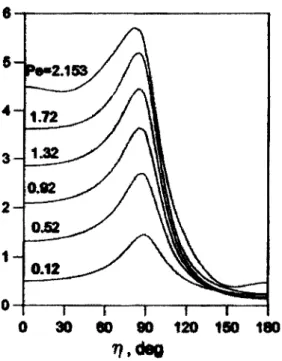
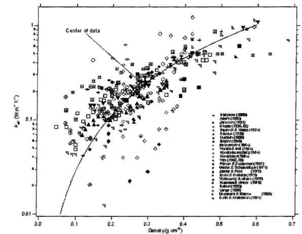
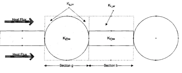
Figure 2-20 Heat-flux distributions obtained for flatness ratio = 0.25 and various Péclet numbers 45 Figure 2-21 Overall HTC at variable Reynolds number 47 Figure 3-1 Measurement of the thermal conductivity of snow. Abel's regression equation (1893) is superimposed on the data for reference (Sturn et ai 1997) 51 Figure 3-2 The published relationship between snow density and thermal conductivity. D, Aggarwal 2004; *, Sturn et al 1997; o, Devaux 1933; A> Snow Hydrology 1956 52 Figure 3-3 Schematic of two types of unit cell inKrischer's model 53 Figure 3-4 Schematic view of snow consisting of ice crystals, water vapor, and air for a

density of 300 kg/m3 57

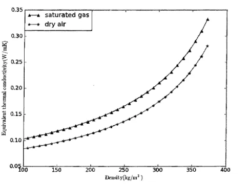
Figure 3-5 Conductivity of ice with respect to temperature 58 Figure 3-6 Thermal conductivity of pure air and gas. A, dry air; o, saturated moist air.... 60 Figure 3-7 Density of air and saturated moist air varies with temperature. A5 dry air; o, saturated moist air 62 Figure 3-8 Ratio of conductivity of ice and saturated moist air varies with temperature ... 63 Figure 3-9 (a) sandwich plate, (b) needle, (c) hollow column, and (d) column with hollow prism facets 64

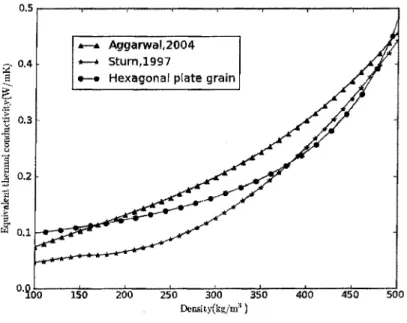
Figure 3-10 A column capped with hexagonal plates 64 Figure 3-11 Geometrical model for hexagonal plate with bond 65 Figure 3-12 Equivalent thermal circuits for snow grain 66 Figure 3-13 Profiles of the equivalent thermal conductivity at -5°C for hexagonal plate grain. A, Satyawali et al (2008); o, Equation 3-18 69 Figure 3-14 Profiles of the equivalent thermal conductivity at -5°C. A, Aggarwal (2004); *, Sturn et al (1997); o, hexagonal plate grain from Equation 3-18 69 Figure 3-15 Profiles of the equivalent thermal conductivity calculated by Equation 3-18 for various snow type at -5°C and ra2 0.0256. A, spherical grain; *, hexagonal plate; o, cylindrical grain; • , cubical grain 70 Figure 3-16 Snow conductivity with (A) and without the effects of (*) water vapor at -5°C

and ra2 0.0256, calculated by Equation 3-18 71

Figure 3-17 Profiles of the equivalent thermal conductivity for snow with cylindrical grain at variable density parameter. A, 300 kg/m3; *, 400 kg/m3; o, 500 kg/m3, calculated by

Equation 3-18 72 Figure 3-18 Profiles of the equivalent thermal conductivity for snow with plate grain at variable density parameter. A, 200 kg/m3; *, 300 kg/m3; o, 400 kg/m3, calculated by

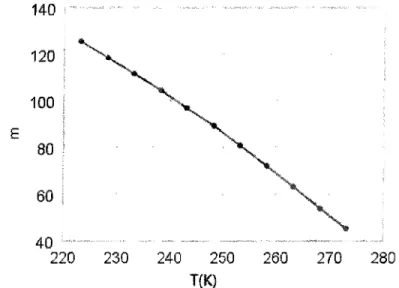
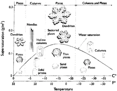
Equation 3-18 73 Figure 3-19 Snow crystal morphology diagram showing types of snow crystals that grow at different temperatures and humidity levels, Nakava(1954) 74 Figure 3-20 Schematic diagram of experimental set-up 77 Figure 3-21 Photo of experiment in process 78 Figure 3-22 Cross-section of a snow sleeve 79 Figure 3-23 Experimental snow conductivity vs density at an air temperature of -4°C. *, experimental data; o, result of Equation 3-18 81 Figure 4-1 Typical plot of the soil-water retention curve from Van Genuchten (1980). The point P on the curve is located halfway between Sr(~ 0.10) andSs ( = 0.50) 91

Figure 4-2 Snow-water retention curve based on the Brook and Corey model (A) and the Van Genuchten (*) model applied to snow 93

Figure 4-3 Relative hydraulic conductivity vs. pressure head as predicted by the Brook and Corey model (A) and the Van Genuchten model (*) applied to snow 94 Figure 4-4 Moisture capacity vs. pressure head as predicted by the Brook and Corey model (A) and the Van Genuchten model (*) applied to snow 94 Figure 4-5 Experiments conducted at the CIGELE laboratories. A, in a cooling room; B, in wind tunnel 96 Figure 4-6 Schematic drawing of the experimental set-up in a controlled climate room... 97 Figure 4-7 Tools for snow sleeve fabrication 98 Figure 4-8 Tools for LWC measurement (A from Roberge, 2006) 99 Figure 4-9 LWC measurement using a fusion calorimeter (Roberge, 2006) 100 Figure 4-10 Photo of snow shedding taken at the CIGELE 102 Figure 4-11 Snow sleeve eroded by strong wind 103 Figure 4-12 Schematic of element used in FEM (A) and FVM (B) 105 Figure 4-13 Triangle-shape used for FEM mesh 106 Figure 4-14 Mesh of the snow sleeve used in FEM 106 Figure 4-15 Water flux at an air temperature of 2°C and a velocity of 4m/s (the origin coordinates are at the sleeve center point) 112 Figure 4-16 Schematic of air gap within snow 114 Figure 4-17 Volume water content varies with time at given locations 116 Figure 4-18 VWC distribution with respect to time. No water flows into or out of the sleeve 117 Figure 4-19 Saturated zone: lower portion of sleeve. Photo taken at CIGELE, 26 January, 2009 118 Figure 4-20 Volume water content distribution at a vertical orientation 119 Figure 4-21 VWC distributions vary with time at an air velocity of 4m/s and an air temperature of 2°C 122 Figure 4-22 VWC at given locations vary with time at an air velocity of 4m/s and an air temperature of 2°C 122

Figure 4-23 Water content variation at given locations at air velocity of 4m/s and an air temperature 2°C 123 Figure 4-24 VWC distribution at 50 s at a series of air velocities and an air temperature of 3°C 124 Figure 4-25 Water content at a given location (x = 0.025, y = 0.025) varies at different air velocities and temperatures 124 Figure 4-26 Time required to reach quasi-steady-state under different air velocities 125 Figure 4-27 VWC distribution at 50 s under a series of air temperatures and an air velocity of2m/s 126 Figure 4-28 VWC at a given location (x = 0.025, y = 0.025) varies at different air temperatures and air velocities 127 Figure 4-29 Time required to reach quasi-steady-state in different temperature conditions 128 Figure 4-30 Volume water content distribution varies with time in seconds at air temperature of 0°C and electric current of 50A 129 Figure 4-31 VWC at a given locations varies with time at an air velocity of 0m/s, air temperature 0° and electric current 50A 129 Figure 4-32 VWC distribution at 50s under a series of electric currents, an air temperature of0°C and air velocity of Om/s 131 Figure 4-33 VWC at a given location (x = 0.0318, y = 0.0227) varies with time for different electric currents at an air velocity of Om/s and air temperature of 0°C 131 Figure 4-34 Water content distribution varies at a set of time interval in seconds at an air temperature of 2°C, an air velocity of 2m/s and an electric current of 50A 132 Figure 4-35 The water content at a given location varies with time at an air velocity of 2m/s, an air temperature of 2°C and an electric current of 50A 133 Figure 4-36 Time required for quasi-steady state at an air temperature of 2°C and a given set of air velocities and electric currents 135 Figure 4-37 VWC variation with time in seconds at roughness 0.035 at an air velocity of 3 m/s and a temperature of 2°C 136

Figure 4-38 Water content variation at 100 s for different roughness r at an air velocity of 3 m/s and a temperature of 2°C 137 Figure 4-39 VWC distribution at 300s for different snow grain size at an air temperature of 2°C and a velocity of 4 m/s 138 Figure 4-40 Comparison of numerical and experimental results for an air velocity of 1.5 m/s and a temperature of 4°C 140 Figure 4-41 Comparison of numerical and experimental results at an electric current of 25A 141 Figure 5-1 A hole during the snow melting period (Photo taken at CIGELE, Jan.27, 2009) 147 Figure 5-2 Wet snow failure photos taken at the CIGELE laboratories 148 Figure 5-3 Schematic of the weakest area of a snow sleeve 149 Figure 5-4 Correlation between the failure strength and the snow density 153 Figure 5-5 Heat transfer at the snow and cable surfaces 156 Figure 5-6 Schematic of water flow under electric heating 159 Figure 5-7 The relationship between/v/>, IVWC, and the heat flux 160

Figure 5-8 fvp increases with increasing IVWC at a given heat flux 161

Figure 5-9 fvp increases with increasing heat flux at a given IVWC 161

Figure 5-10 Schematic of the water flow under forced convection 162 Figure 5-11 The relationship between/VjP and IVWC, forced air convection 163

Figure 5-12 fvp increases with increasing IVWC at a given heat flux 163

Figure 5-13 fvp increases with increasing heat flux at a given IVWC 164

Figure 6-1 Temperature distribution along the surface of the sleeve 174 Figure 6-2 Heat flux around the surface of the sleeve 175

Table 2-1 Boundary conditions assigned in FLUENT 20 Table 2-2 Reynolds number at different air velocities 21 Table 2-3 Turbulence intensity 24 Table 2-4 Constants of Equation 2-1 29 Table 2-5 Overall average Nu for a circular cylinder 29 Table 2-6 Roughness parameters 31 Table 2-7 Overall average Nusselt number 37 Table 2-8 Ellipse parameters 41 Table 2-9 JVn for circular and elliptical cylinder 46 Table 2-10 Overall HTC at variable Reynolds number 47

Table 3-1 Shape Factors Ag 67

Table 3-2 Relationship between temperature and parameter ra2 68 Table 3-3 Weather and models (for fresh snow) 75 Table 3-4 Abbreviation of Models 75 Table 3-5 Weather and models (for accumulated snow) 76 Table 4-1 Heat and water flux at the conductor surface 113 Table 4-2 Microstructure of snow and residual water height 114 Table 4-3 Snow properties in the initial state 115 Table 4-4 Time to quasi-steady state under electric heating 130 Table 4-5 Time required for quasi-steady-state at given air temperatures and a given set of air velocities and electric currents 134 Table 4-6 Time required to reach a quasi-steady-state under different roughnesses (at a velocity of 3 m/s and a temperature of 2°C) 137

Table 4-7 Time to quasi-steady state at an air velocity of 4 m/s and a temperature of 2°C 139 Table 4-8 Initial values for the experiment 139 Table 4-9 Initial values for the experiment 141 Table 5-1 Heat flux at the conductor surface at 0°C (ACSR diameter 12.7 mm) 157 Table 5-2 Heat flux at the snow sleeve surface (diameter 0.1 m) 157

LIST OF SYMBOLS

Area of domain under study Semi-minor axis Moisture capacity Roughness constant Deformation factor Diameter Ellipse eccentricity Ellipse flatness ratio Gravitational acceleration Geometry

Heat transfer coefficient Height of snow grain Pressure head Turbulence intensity Electric current Thermal conductivity

Equivalent thermal conductivity Intrinsic permeability Dimensions m mz m 1/m m m/sz W/m^K m m A W/mK W/mK mz

K Ks 1 L M Nu P Pr q Q r R R Re Ree S Se t T Uavg V V

w

Relative permeability of water Saturated hydraulic conductivity Roughness Height Length of bond Latent heat Mass Nusselt number Pressure Prandtl number Heat flux Heat transfer rate Roughness Constant Radius

Thermal resistance Reynolds number

Turbulent Reynolds number Water saturation

Effective water saturation Time

Temperature Mean flow velocity Velocity Volume Liquid flux m/s m m J/kg kg Pa W/mz W M m'K/W s K o r ° C m/s m/s m* nrVs

Greek Symbols a

P

e

Dynamic viscosity Mass density Stress Shear stress

Pore water pressure head Porosity m'/s Degree Degree Ns/mz kg/mJ Pa Pa m Subscripts a b e f g i m s w Dry air

Bond between snow grain Equivalent or effective Film

Failure

Saturated moist air Ice

Melting point Surface Snow Water

INTRODUCTION

1.1 Defining the Problem

In general, it has been considered that snow accretion on overhead power lines occurs only when wet snowflakes adhere to wires at surface temperatures slightly above freezing. Sakamoto (2000) suggested that, in practice, the phenomenon of snow accretion may customarily be experienced under a relatively wide range of combinations of meteorological parameters. The observation records show that the snow accretion on overhead wires may occur at air temperatures as low as -7°C.

Wet snow accretion, as reported by Colbeck et al (1982), is known to be particularly troublesome since a large mass accumulation can occur in only a few hours. Snow accretion on overhead transmission lines and wires may thus be deemed a serious problem posing tremendous threats to existing power installations. Its subsequent shedding tends to cause power outages and severe damage to the power network structures, thereby leading to a number of serviceability, safety, and mechanical reliability issues.

Germany, Norway, Iceland, and Japan experience wet snowfalls which affect the related overhead transmission networks. The damage caused by a single wet snowstorm can necessitate the expenditure of sums on the order of 100 million dollars. Past records show that the occurrence of wet snow accretion is relatively more common and may be equally as catastrophic in France, Japan, and Iceland.

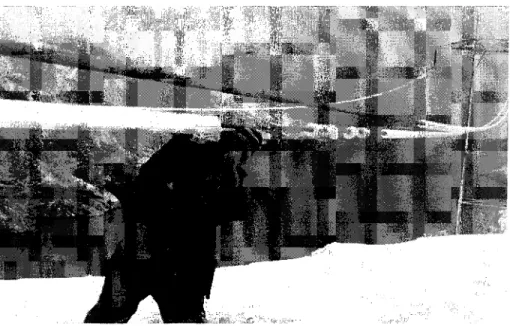
The shape of a snow sleeve accreted on overhead lines depends not only on meteorological parameters such as air temperature and velocity, but also on line parameters such as material and stranding. The snow sleeves taken under observation were usually almost cylindrical due to the effects of wind flow and cable torsion (Wakahama et al, 1977, Admirât, 1988, Yukino, 1998), as shown in Figure 1-1.

Figure 1-1 Wet-snow accretion on a 300 kV power line in Dale-Fana, Norway (Photograph from Satnett)

consequently not well documented. Few people have actually witnessed the phenomenon, while observations tend to be varied and scattered.

In order to minimize the damage, the physics of snow-shedding, as well as the effect of the different factors which influence snow shedding, are both important areas of research.

A satisfactory theoretical model for snow shedding from overhead lines is not yet readily available, even though extensive studies on snowing phenomena have been carried out to date by researchers in the domain. There are several factors existing which hamper research and investigation into the snow-shedding process.

• The complexity of the snow-shedding phenomenon itself. The shedding involves several feedback mechanisms and non-linear relationships between various factors, including the fact that ambient forced or natural air convection depends on the air temperature and velocity as well as on the shape of the snow sleeve and its surface roughness; and that water percolation within the snow not only depends on but also transforms the snow micro structure.

• The difficulty of predicting and measuring snow morphology. Significant characteristics of the snow micro structure involve the arrangement of snow grain, pores, and possibly liquid water; they tend to change dynamically due to water percolation within the snow, or as a result of such environmental effects as air convection. Snow-grain morphology is one of the most important parameters for predicting snow failure, or shedding. This parameter strongly influences the

methods available at present for observing the morphology of wet snow (Dozier, 1987; Brun, 1991).

• The lack of experimental data. Snow shedding under natural conditions is rarely observed. A method developed by Roberge (2006) was used to reproduce wet-snow sleeves in a cold chamber or wind tunnel. There are considerable technical problems involved in measuring accurately these quantities such as liquid water content, however, even under laboratory conditions.

The study of snow-shedding mechanisms poses a genuine challenge, considering the paucity of studies in the overview of the literature.

1.2 Research Objectives

The general objectives of this study include developing models which simulate the snow melting process within a wet snow sleeve and which also predict snow-shedding under various meteorological conditions or the current prevailing transmission environment.

Heat tranfer coifficient computation snow surface Thermal balance of melted water production on sleeve surface Water percolation simulation Water percolation No Snow shedding prediction

Figure 1-2 Research objectives and modeling procedure

A. Analysis of the Convective Heat Transfer around a Snow-Covered Conductor An assessment of the overall Heat Transfer Coefficient (HTC) and local HTC distribution for a snow sleeve is required in order to complement the snow-melting model. Therefore, the objective of this part of the study is to determine the convective heat transfer coefficients around a snow sleeve in a cross-flow of air.

1-3. As a result, the air velocity distribution around the sleeve will change continually and will lead to variation in the local convective heat transfer rate.

Figure 1-3 Creep progressions up to shedding (from Roberge 2006)

Not only has the shape of the snow sleeve influenced local HTC distribution, but also the status of the snow surface. The sleeve surface status is the research emphasis in this present study.

A snow sleeve has a relatively higher water content before snow shedding occurs. It is, therefore, reasonable to assume that the greater part of the sleeve surface is at a constant temperature, 0°C, while most prior experiments were conducted in a situation of constant heat flux from the surface.

B. Analysis of the Water Percolation within the Snow Sleeve

Wet snow was classified into two basic modes, or regimes, based on liquid water saturation: the pendular and the fimicular. At low LWC values (Figure l-4a), the water forms pendular rings at the points of contact between the particles, and the air is connected

connected; this is known as the funicular regime (see Figure l-4b). \ Air

O

r

Figure 1-4 Wet snow in the (a) Pendubr and (b) Funicular regimes. Reproduced from Armstrong et al (1976)

Water percolation in snow is of fundamental importance in snow hydrology. Snow melting and water percolation are dynamic, evolutionary processes, however, and they are indeed quite complicated. The geometry of a snow sleeve with a hole produced by a line conductor is even more complex and is thus unsuitable for a one-dimensional model. For this reason, the mechanism study will pose a genuine challenge.

The water percolation within the snow sleeve depends not only on the initial water saturation but also on the microstructure of wet snow, including porosity, snow grain size and shape, which are all affected by the concurrent heat exchange between the water, air, and ice matrix. The wind velocity, air temperature, Joule heating, and snow surface roughness have an evident influence on the rate at which snow melts.

water percolation within a wet snow sleeve.

C. Determining the Equivalent Conductivity of Dry Snow

For snow, which is composed of various substances in different states, heat transferred by conduction may occur in several forms. As temperature changes, snow exhibits a dynamically complex process represented by three fractions continuously changing their ratios: ice particles, water, and the gaseous phase (including air and water vapor). Based on an elegant experiment designed by de Quervain (1958, 1972) it was estimated that the ice matrix for snow samples carried 55-60% of the heat, the rest moving across the pores as sensible or latent heat. Reviewing the literature on vapor diffusion in snow, Colbeck (1993), concluded that 30-40% of the heat is moved by vapor transport because the vapor gradient enhancement predominates over the blocking effect of the ice matrix.

The thermal characteristics of snow depend upon various factors such as the thermal conductivity of constituent phases, porosity, shape and size of snow grain, and so forth. A microstructure model have a conceptual understanding of the snow structure and take into account the influence from geometry of snow grain and connection bond.

An assessment of the equivalent thermal conductivity of snow is required in order to complete the snow melting and shedding model. The objective of this part of the study is to determine the equivalent thermal conductivity of dry snow, especially for the snow accreted on an overhead cable.

Snow is a complex material with unique properties including high compressibility and thermodynamic instability. It is, therefore, not surprising that the failure mechanisms of wet snow shedding are not well understood, and that they are in fact, controversial.

A great number of studies have been carried out on dry snow failure, but wet snow shedding is more complicated. The water within the wet snow may incline or decline snow shedding according to snow porosity. Water percolation has an evident effect on snow shedding, in that it changes the size and shape of snow grains as well as the bonding connection between neighboring snow grains.

The objective of this portion of the work is to develop a mathematical model for predicting the occurrence of snow shedding based on the experimental data obtained at the CIGELE laboratories. This model is able to provide a rapid estimation of the Joule heat or wind required to trigger snow shedding from the cable.

1.3 Methodology

This research project will be carried out in such a way as to ascertain that theoretical modeling or numerical simulation is followed by the type of experimental investigation which will produce the relevant data for validating the preceding modeling procedures.

Two-dimensional State Reynolds-Average Navier-Stokes (RANS) simulations are here implemented in a commercial computational fluid dynamic software package, FLUENT, to facilitate predicting both the overall heat-transfer rate and the local heat-transfer coefficient distribution along the snow sleeve surface subsequently.

Firstly, a set of elliptical shapes were investigated and their values compared with the values obtained from the circular cylinder shape.

Secondly, in carrying out the above, the surface roughness of a circular cylinder sleeve was taken into account. A variety of roughness values were investigated and compared with each other under the same Reynolds number conditions.

The computational results were then compared with the theoretical analyses and experimental data from the literature in the field.

B. Analysis of Water Percolation within the Snow Sleeve

A two-dimensional Finite Element Method (FEM) and a Finite Volume Method (FVM) time-dependent model were both built to simulate melted-water percolation within a snow sleeve under the different prevailing snow properties and outer environment conditions.

With the above-declared intention, the effects of wind velocity, air temperature, Joule heating, snow surface roughness, and snow grain size were all investigated and analyzed.

The experimental study was carried out to validate the numerical approaches as well as to acquire a better understanding of the water percolation process within a snow sleeve.

Wet snow sleeves were reproduced and the variations of liquid water content and snow density were recorded.

C. Determining the Equivalent Thermal Conductivity of Dry Snow

A microstructure model was developed to estimate the quantitative relationship between the equivalent thermal conductivity and the constituents of dry snow.

First, the shape of the snow grain was classified into four main types and a micro structure model was developed to estimate the equivalent conductivity and density of the snow sleeve. Second, a study was made of the dependence of the thermal conductivity on such snow constituents as air, ice, and vapor, as well as on the effects of the temperature. Third, a set of experiments was conducted and a comparison was made with the results of the analytical model. The temperature gradient were measured within a dry snow sleeve. Lastly, the relationship between snow microstructure and the prevailing weather conditions was presented.

D. Prediction of Wet Snow Shedding from an Overhead Line Conductor

A dry snow failure model was revised and extended to apply to wet snow shedding from an overhead line conductor. The effective initial water content, in the form of a custom-defined parameter, was introduced, accounting for the effect of the water percolation within the snow sleeve.

With regard to the melted water percolation, the outer conditions were subdivided into two types: forced air convection and Joule heating with natural air convection. Under the former conditions, melted water percolates throughout all areas within the snow sleeve and the rate of snow melting is not consistent due to local HTC variation along the snow sleeve surface. Under the latter conditions, melted water concentrates on the lower section of the snow sleeve.

Wet snow sleeves were reproduced and the occurrence of snow shedding were recorded at the CIGELE laboratories. The experimental data are used to fit the value of the parameters in this empirical model.

CHAPTER 2

A NUMERICAL STUDY OF HEAT CONVECTION AROUND

A SNOW SLEEVE IN A CROSS-FLOW OF AIR

2.1 Introduction

Snow accretion on overhead transmission lines and ground wires can lead to a number of serviceability, safety, and mechanical issues. In order to develop methods for preventing snow accretion or shedding from overhead conductors, it is necessary to estimate the heat transfer and flow characteristics around snow sleeves from the point of view of various engineering aspects. For example, convective heat transfer plays a significant role in the thermal balance for snow melting and refreezing processes.

The air flow around a circular cylinder at a high Reynolds number (Re) has long been the subject of intense attention from academic and practical standpoints. This flow is concerned with the complicated interaction between the transition and separation of the boundary layer on a rounded surface. A large number of studies were carried out by numerous investigators, and several empirical correlations were developed for the heat transfer coefficient.

Considering that a snow sleeve is not always a perfect cylinder, however, it is necessary to make a specific study of snow sleeves in this respect.

This chapter presents the results of a numerical investigation into the effects of the special characteristics of a snow sleeve, including surface roughness and non-circular shape, on the local HTC distribution around the sleeve under different wind conditions.

1. Non-Circular Shape

During the snow melting process, the outer shape of the sleeve changes continuously due to the melted water flow, the metamorphism of the ice matrix within the snow, and so forth.

For the purposes of this investigation, a set of elliptical cylinders was simulated in a cross flow of air. The numerical results were compared with those for circular cylinders.

2. Roughness

In prior works, the snow sleeve was assumed to have a smooth surface but, in actuality, it has a rough surface. Micro-reliefs on the snow surface are formed by a process of erosion and snow redeposition by the wind.

Normally, increasing the roughness increases the heat transfer rate in the turbulent boundary layer and, in addition, causes the transition from a laminar to a turbulent layer to occur earlier.

A total of 10 wind scenarios were simulated in FLUENT. The wind varies from 1 to lOm/s, and the Reynolds number from 7400 to 74 000. Three typical scenarios are presented here.

2.2 Review of the Literature

The air flow past a circular cylinder at a high Reynolds number has long been the subject of intense attention from academic and practical studies. This subject is concerned with the complicated interaction between the transition and separation of the boundary layer on rounded surfaces. Numerous studies have been carried out and several empirical correlations have been developed for the heat transfer coefficient.

The local and overall heat transfer coefficient (HTC) can be determined by:

• experiments ( traditional electrical heating method, optical method)

• numerical calculations ( using finite volumes, differences and element methods)

As is well known from the literature, the laminar boundary layer over the front stagnation point of a cylinder in a cross-flow is the thinnest and its thickness increases with downstream displacement. Separation of the laminar boundary layer takes place when the low velocity fluid close to the cylinder wall cannot overcome the adverse pressure gradient over the rear portion of the cylinder and the flow eventually stops and begins to move in the opposite direction (Incropera et al, 2002). Fluid movement starts to curl and gives rise to vortices that shed from the cylinder. The Nusselt number then increases as a result of the intense mixing in the separated flow region, called the wake.

The complicated flow pattern across a cylinder greatly influences heat transfer. Giedt (1949) proposed an experimental schematic to measure the variation of local HTC along the circumference of a circular cylinder in a cross-flow of air. Achenbach (1975), Zhukauskas (1985), Scholten et al (1998) and Buyrul (1999) also presented the distribution of local HTC along a circular or elliptical surface by means of well-designed experiments. Figure 2-1 describes simultaneous measurements of time-resolved heat flux at the surface of a cylinder in a cross-flow through wind tunnel experiments by Scholten et al (1998).

7190

è » 60 90

An g I « ( d 0 g )

Figure 2-1 Surface Nusselt number by Scholten et ai (1998)

The complicated nature of the cross-flow around the bluff body makes it an excellent case for assessing the ability of computational software to reproduce real flow conditions. FLUENT and CFX are popular programmes used to simulate the process of air flow and heat transfer.

A modified k-co turbulence model proposed by Durbin (1993, 1996) was implemented in FLUENT by Szczepanik et al (2004). The modification arose from the unfortunate tendency of two equation turbulence models to over-predict levels of turbulent kinetic energy close to a stagnation point. Figure 2-2 shows the Nu profiles for a given Reynolds number studied, including the experimental data from Scholten et al (1998) and also considering the overall comparison between the experiment and the simulation.

450 400 350 300 et 200< 150 too SO fi se 'm. '-1 -T X x **•*"* ^ — — -\ X \ \ * \ x x- \ y Experîmenial - Steady State: fc-w - Steady State: T - limit k-w

X"—"\ // / f —"~*k.j>^ « : * 1 * : * 1 . : * t î : * 1 * : * 20 40 60 100 120 140 160 180 200 angle ite$

Figure 2-2 Surface Nusselt number for Re = 50350 by Szczepanik et al (2004) Péter (2006) conducted an intensive study on heat exchange around a circular cable. He utilized the Finite Volume Method (FVM) to study the relationship between the local HTC distribution and the Reynolds numbers.

Little work is known to have been carried out for cylinders with rough surfaces. Elmar (1977) and Achenbach (1977) designed a series of tests to obtain local heat transfers on

rough surfaces and Makkonen (1985) developed a mathematical boundary-layer model to predict the local HTC distribution along rough cylinder surfaces.

2.3 Modeling in FLUENT 2.3,1 Geometry

The snow sleeve was modeled as a circular or elliptic cylinder while a square flow domain was created around the cylinder, as shown in Figure 2-3. A uniform velocity at the inlet of the flow domain can thus be specified.

The general procedure for solving the problem is:

a) create the geometry (cylinder and flow domain) b) set the material properties and boundary conditions c) mesh the domain

d) carry out the computation in FLUENT e) analyze the results.

A flow domain was created surrounding the cylinder. The upstream length is 15 times the radius of the cylinder, and the downstream length is 40 times the same radius, while the width of the flow domain is 50 times that radius. To facilitate meshing, a square with a side length of 6 times the radius of the cylinder was created around the cylinder. The square was then split into four pieces, as shown in Figure 2-3.

inlet Side Boundary 15R Side Boundary Outlet 40R

Figure 2-3 Air flow domain schematic

2.3.2 Mesh

The edges were meshed using the First Cell Height and the calculated number of intervals. The entire domain was meshed using a map scheme (Figure 2-4). Only the upper part of the domain was selected in order to save computing resources.

A boundary layer with 12 rows was placed at the cylinder wall using the calculated value of First Cell Height.

Figure 2-4 Partial schematic of a domain mesh

2.3.3 Boundary Conditions

The boundary conditions were assigned in FLUENT as shown in following table.

Table 2-1 Boundary conditions assigned in FLUENT

Boundary Cylinder Inlet Side boundaries Outlet Assigned As Wall Velocity inlet Symmetry Pressure outlet

2.3.4 Reynolds Numbers and Flow Classification

Table 2-2 provides the Reynolds numbers for airflow under different air velocities. The

Table 2-2 Reynolds number at different air velocities Velocity (m/s) 1 2 3 4 5 6 7 8 9 10 Reynolds number 7407 14815 22222 29630 37037 AAAAA 51852 59259 66667 74074

Based on the Reynolds numbers, the following physical models are to be recommended:

• Re < 1000 laminar flow

• 1000 <Re <10000 low Reynolds number k-co model or k-e model • Re> 10000 k-o) model or k-s model

At higher Reynolds numbers, and as presently investigated, the wake of the boundary layer becomes turbulent, a turbulence model should thus be chosen. Two-equation models such as the k-m model or the k-e families offer the ability to introduce turbulence into the flow.

2.3.5 Turbulence Models

For numerical solutions of the Reynolds-averaged Navier Stokes equations, the commercial Computational Fluid Dynamic (CFD) software package, FLUENT, was used. FLUENT uses the finite volume method (FVM) to solve the governing equations sequentially. Several turbulence models were used in this study. From among these, the results obtained from the shear stress transport (SST) k-w model show better agreement when compared to the experimental data.

The SST k-(o turbulence model utilizes a calculation of turbulent viscosity based on the standard k-a) model. Thus, the closure coefficients and other relations also differ slightly. Nonetheless, the SST k-a) turbulence model may be considered the standard or unmodified turbulence model for the current study.

The SST k-co model was developed by Menter to blend the robust and accurate formulation of the k-co model effectively in the near-wall region with the free-stream independence of the k-o) model in the far field. To achieve this, the k-co model was converted into a k-(o formulation. The SST k-m model is similar to the standard k-omega model, but includes the following refinements.

1. The standard k-a> model and the transformed h-e model are both multiplied by a blending function and both models are added together. The blending function is designed to be one in the near-wall region, which activates the standard k-w model, as well as zero, away from the surface, which activates the transformed k-s model.

2. The SST model incorporates a damped cross-diffusion derivative term into the œ equation.

3. The definition of the turbulent viscosity was modified to account for the transport of the turbulent shear stress.

4. The modeling constants are different.

These features make the SST k-w model more accurate and reliable for a wider class of flows (e.g., adverse pressure gradient flows, airfoils, transonic shock waves) than the standard k-co model. Other modifications include the addition of a cross-diffusion term in the co equation and a blending function to ensure that the model equations behave appropriately in both the near-wall and far-field zones.

2.3.6 Determining Turbulence Parameters

The flow across the snow sleeve was solved as an incompressible problem with air being the fluid. Pressure discretization was set by using the Standard and other Second Order Upwind. This coupled method was adopted for pressure-velocity coupling.

In most turbulent flows, higher levels of turbulence are generated within the shear layers which enter the domain at the flow boundaries, making the result of the calculation relatively insensitive to the inflow boundary values. Nevertheless, caution must be used to ensure that boundary values are not so unphysical as to contaminate the solution or impede the convergence. This is particularly true of external flows where unphysical large values of effective viscosity in the free stream can "swamp" the boundary layers.

The turbulence specification methods described above can be used to enter uniform constant values instead of profiles. Alternatively, the turbulence quantities in terms of more convenient quantities such as turbulence intensity, turbulent viscosity ratio, hydraulic diameter, and turbulence length scale may be specified.

23.6.1 Turbulence Intensity

The turbulence intensity, /, is defined as the ratio of the root-mean-square of the velocity fluctuations, u\ to the mean flow velocity, uavg.

To match experimental values, inlet / a t different Reynolds numbers was set as follows:

Table 2-3 Turbulence intensity

Re 1401 29630 59259 / 1.6% 0.4% 0.32%

2.3.6.2 Turbulent Viscosity Ratio

The turbulent viscosity ratio, fit/ft, is directly proportional to the turbulent Reynolds number (Ret = k*/(£v)). The Ret is large, on the order of 100 to 1000, in

high-Reynolds-number boundary layers, shear layers, and fully-developed duct flows.

However, at the free-stream boundaries of most external flows, fit /fi is fairly small.

2.4 Heat Transfer around a Circular Smooth Surface Cylinder

2.4.1 Flow Properties

2.4.1.1 Velocity Distribution

The contours of velocity are shown plotted in Figure 2-5. It may be seen that, from the front stagnation point, the air velocity increases with 0 and the maximum velocity occurs at

0 ~ 80° (red area).

Figure 2-5 Contours of vetacity at inlet velocity = 8m/s

2.4.1.2 Local Static Pressure

As shown in Figure 2-6 and Figure 2-7, the free stream fluid is brought to rest at the frontal stagnation point, with an accompanying rise in pressure. From this point, the

pressure decreases with increasing i/5 the streamline coordinate, and boundary layer

develop under the influence of a favorable pressure gradient (dp/dq <0), where tj is the streamwise coordinate measured along the surface. The pressure eventually reaches a minimum, however, and towards the rear of the cylinder, further boundary layer development occurs in the presence of an adverse pressure gradient {dp/dtj >0).

Stagnation Point Separation Point

^Boundary Layer

Figure 2-6 Sketch of the flow field around a cylinder in cross flow

Static Pressure (pascal) S.QDe+Ql -4.ÛÛe+ûi ^ 3,00^+01 2,0De+Ql LGDe+01 LOQe+Ql --2,0Be+Ql : 3.0De+Ql --4.ÛÛÔ+ÛI -Q.D6 -0,04 -8.(12 0 0.0H Position (m)

Figure 2-7 Static pressure distribution abng sleeve surface at inlet velocity v = 8m/s [the origin

2.4.2 Local HTC Distribution

In general, all cases indicate the correct characteristic shape of the local Nusselt number

(Nu) around the circular cylinder. In the subcritical range (Re<lO5)9 a local maximum of

the Nu is located at or close to the stagnation point, and the Nu decreases when 0 increases as a result of laminar boundary layer development. A minimum Nu is reached close to the top of the cylinder, at 6 ~ 80°, which is associated with separation. Moving further into the wake region, Nu increases with 0 due to mixing associated with vortex formation (Incropera, 2007).

250 r

20 40 60 80 100 120 140 160 180 Angular coordinate 8

60 80 100 120 140 160 180 Angular coordinate 8

Figure 2-9 Local HTC at variable Re: +, Re = 7407; A, Re = 29630; o, Re = 59259 Figure 2-8 and Figure 2-9 show the Nu profile from the numerical results for the smooth surface cylinder, i.e. K/d - 0. The horizontal axis is a circumferential angle in degrees, where 0 degrees is the leading edge or front stagnation point of a cylinder, and 180 degrees is the trailing edge or rear. The diameter of the circular cylinder is 0. lm.

2.4.3 Overall HTC

The empirical equation from Hilpert is

Equation 2-1 where the constants C and m are listed in Table 2-4 for Re value ranges.

Table 2-4 Constants of Equation 2-1 ReD 4000-40,000 40,000-400,000

c

Churchill and Bernstein have proposed a single comprehensive equation which is valid for a wide range of Reynolds numbers (Ren) and Prandtl numbers. The equation is recommended for all Re^Pr > 0.2 and has the form

NUn = 0.3 + i Equation 2-2

The assumed condition is that the surface temperature is 0°C and the ambient air temperature is 3°C. In Equation 2-1 and Equation 2-2, the air properties are evaluated at the film temperature of 1.5 degrees.

Tf = _{Equation 2-3}

where Tf is the film temperature, Ts is the surface temperature, and Ta is the air

temperature.

Table 2-5 Overall average Nu for a circular cylinder Air Velocity(in/s) 1 4 8 Reynolds Number 7407 29630 59259 ^«(Equation 2-1) 42.90 101.04 169.85 7V«(Equation 2-2) 46.00 101.06 154.91 iVK(numerical) 39.59 86.46 133.03

Table 2-5 compares the average Nusselt numbers obtained from empirical Equation 2-1, Equation 2-2 and the numerical simulations. It may be observed that the numerical results are about 15% less than those obtained from the empirical equations. The reason for this discrepancy is that the simulations were carried out at a constant surface temperature, while most experiments were conducted in a constant heat flux from the surface.

Considering that mixtures of ice particles and water are produced during the snow melting process, it is therefore better to choose a model at a constant surface temperature of 0°C.

2.5 Local HTC Distribution for Rough Surface Cylinders 2.5.1 Roughness of Snow

The roughness of a snow surface is caused by wind, uneven evaporation, or uneven melting. Lacroix et al (2008) investigated snow pack and found that the roughness of snow varied largely as a result of weather and geographical conditions. Even for relatively smooth surfaces, the classical roughness parameters are found to be in the 0.5-9.2 mm range for the RMS height distribution. For more detailed information on the rough surface effects, a set of values is listed in Table 2-6.

To model the wall roughness effects, two roughness parameters must be specified: the Roughness Height, Ks, and the Roughness Constant, CKS> The default roughness height (Ks)

is zero, corresponding to smooth walls. For snow types of roughness, it is recommended that an "equivalent" sand-grain roughness height should be used for Ks.

Choosing a proper roughness constant (Cj&) is dictated mainly by the type of the given roughness. The default roughness constant (G& = 0.5) was recommended by FLUENT to simulate for uniform sand-grain roughness and computation convergence.

The roughness factor, r is defined as ratio of roughness height, Ks and the diameter of

snow sleeve, D and shown in Table 2-6. The diameter of snow sleeve is assumed as 0.1 m in this study.

r = D Equation 2-4

Table 2-6 Roughness parameters

* ( m ) 0.000075 0.00009 0.0001 0.0005 0.001 0.002 0.003 0.004 D(m) 0.1 0.1 0.1 0.1 0.1 0.1 0.1 0.1 i-(xl0"J) 0.75 0.9 1 5 10 20 30 40 2.5.2 Pressure Distribution

The local static pressure distribution around the circumference of a rough cylinder is shown in Figure 2-10. The static pressure was plotted against the angle from the front stagnation point, while the Reynolds number appears as a parameter. The pressure is normalized by the following equation.

Pe =

P-Pcc

Equation 2-5 For subcritical flow conditions, the pressure minimum is located at about 0 = 70° and it decreases with increasing Re.

Figure 2-11 represents the pressure distribution at a constant Reynolds number for variable roughness parameters. It may be found that the lower roughness (r < 9xlO"3) does not affect the pressure distribution. The maximum value of the adverse pressure increases obviously when the roughness is greater than 9x 10"3.

1 0.8 0.6 0.4 0.2 0 -0.2 -0.4 a a o a tf -0.6 -0.8 -1 40 60 80 100 120 140 160 180

Figure 2-10 Local static pressure distribution at r = 3*10-3 and variable Re parameter. *, Re = 7104; o,Re = 22222

0 20 40 60 80 100 120 140 160 180

Figure 2-11 Local static pressure distribution at Re = 6.67xl04and variable roughness parameter. *, r = 0, smooth surface; A, r = 2x10-3; o, r = 11x10-3; 0, r = 15x10-3 2.5,3 Local HTC Distribution

In Figure 2-12, Figure 2-13, and Figure 2-14, the local heat-transfer distribution around a cylinder was plotted for each Reynolds number. The varied parameter here is surface roughness. The Nusselt number is normalized by Re'm.

Figure 2-12 shows the results for the smallest Reynolds number, Re = 7407. It may be seen that most of the effects caused by surface roughness occur in the wake range of the air flow. Even at the highest roughness value, r - 50xl0~3, the minimum Nu is still at almost the same position as it is for a smooth surface.

20 40 60 80 100 120 140 160 180 Angular coordinate 8

Figure 2-12 Local HTC at Re = 7407 and variable roughness parameter. +, r = 0, smooth

surface; A, r = 10*103; o,r = 30x10-3;*,r = 40x10-3;x, r = 50x10-3

20 40 60 80 100 120 140 160 180 Angular coordinate $

Figure 2-13 Local HTC at Re = 2.2xlO4 and variable roughness parameter. +, r = 0, smooth

20 40 60 80 100 120 140 160 180 Angular coordinate $

Figure 2-14 Local HTC at Re = 6.67xlO4 and variable roughness parameter. +, r = 0, smooth surface; A,r = 3x10-3; o, r = 9xlO-3;*,r = 12x10-3;x,r = 15x10-3

Figure 2-13 exhibits the results for a higher Reynolds number, Re = 22222. In a lower roughness range r < 2xlO"2, the curves have similar shape characteristics: the boundary layer is laminar throughout, and its separation is indicated by a minimum near 0 = 80°.

When the curve is associated with a higher roughness value, r = 30x 10"3 is compared to the one with a smooth surface and the difference is largely apparent. There is a direct transition from the laminar to the turbulent boundary layer at 50° which generates high heat transfer coefficients downstream because the heat transfer in the turbulent flow is more effective than in the laminar flow. In the turbulent region, Nu increases with increasing 0 until it reaches its maximum value at around 0 ~ 70°, and then decreases. The separation occurs at 0 ~ 110°. The curve r = 35xl(T3 shows similar behavior with the exception of the

fact that the transition point is at 0 ~ 40° and the peak value of the Nusselt number is approximately 23% higher.

Figure 2-14 qualitatively shows similar results for the local heat transfer at Re - 66667. Comparing Figure 2-14 and Figure 2-13, it may be observed that as the roughness parameter increases, the laminar-turbulent transition occurs at a decreasing Re. These results are consistent with Achenbach's experiments (1977).

The values of heat transfer at the front stagnation point would be expected to be equal to unity, considering that the flow near the stagnation point is laminar. Some experimental results are greater than unity mainly because of the limitations of laboratory equipment.

At a given Reynolds number, it may be observed that:

• the greater the roughness, the closer the laminar-turbulent transition point approaches the front stagnation point;

• the peak value of Nu increases upon increasing the roughness parameter;

• the location of the Nu peak value moves closer to the front stagnation point with increasing roughness;

• the heat transfer within the wake region increases with increasing roughness.

2.5,4 Total Heat Transfer

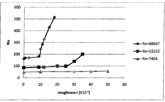
Figure 2-15 exhibits the overall average Nusselt numbers at different roughness values. It can be seen that the total heat-transfer increases with the surface roughness. After the

roughness parameter exceeds a critical value, heat transfer increases more intensely. But, at a lower Re, there is no such critical value while r < 0.05.

Table 2-7 Overall average Nusselt number

Roughness r^lO"3) 0 3 9 10 11 12 15 18 20 25 30 35 40 50 Re = 7407 47.60 52.19 53.86 54.98 56.32 Re = 22222 85.91 90.22 90.33 99.7 98.99 139.58 199.98 Re = 66666 161.45 170.11 182.21 242.26 286.61 326.83 429.46 514.65

600 500 400 300 100 n U

J

/

/

f

f

T

f

Figure 2-15 Overall average HTC at variable roughness

2.6 Local HTC Distribution for an Elliptical Cylinder 2.6.1 Elliptical Cylinder: Definition

An ellipse is a smooth closed curve which is symmetric about its center. The distance between antipodal points on the ellipse, that is to say the pair of points whose midpoint is at the center of the ellipse, with a maximum and minimum along two perpendicular directions, namely the major axis, or transverse diameter, and the minor axis, or conjugate diameter, respectively. The semi-major axis or major radius, denoted by a in Figure 2-16, and the semi-minor axis or minor radius, denoted by b in Figure 2-16, are one half of the major and minor diameters, respectively.

Figure 2-16 Definition of ellipse 1. The eccentricity of the ellipse is

e = I — I —

2. The flatness ratio is defined as

Equation 2-6

Equation 2-7 3. The area enclosed by the ellipse is

A = _{Equation 2-8}

where a and b are one-half of the major and minor axes of the ellipse, respectively. Circumference

The circumference C of an ellipse is 4aE(e), where the function E is the complete elliptic integral of the second kind. A good approximation of circumference is Ramanujan's equation:

Equation 2-9 2.6.2 Snow Sleeve Deformation

It is customarily assumed that the cross section of the snow sleeve remains constant during the snow melting process. The deformation factor may thus be defined as

d = — Equation 2-10

where R is the radius of the circular cylinder and A/ is the variation length for the semi-minor radius of the ellipse.

Therefore, it is possible to obtain the semi-minor radius by

b = R x ( l - d ) Equation 2-11 and the semi-major radius by

a = A/Or x a) Equation 2-12 The parameters of a set of ellipses are listed in Table 2-8. From this, it is clear that the perimeter of an ellipse increases with its eccentricity.

It should be noted that snow sleeve becomes deformed as a bluff shape, Le. when the minor axis is perpendicular to the flow.

Table 2-8 Ellipse parameters Deformation 1% 2% 3% 4% 5% 6% 7% 8% 9% 10% 20% 30% Circle Radius 0.05 0.05 0.05 0.05 0.05 0.05 0.05 0.05 0.05 0.05 0.05 0.05 Area 0.0079 0.0079 0.0079 0.0079 0.0079 0.0079 0.0079 0.0079 0.0079 0.0079 0.0079 0.0079 Perimeter 0.31 0.31 0.31 0.31 0.31 0.31 0.31 0.31 0.31 0.31 0.31 0.31 Ellipse a 0.0505 0.0510 0.0515 0.0521 0.0526 0.0532 0.0538 0.0543 0.0549 0.0556 0.0625 0.0714 b 0.0495 0.0490 0.0485 0.0480 0.0475 0.0470 0.0465 0.0460 0.0455 0.0450 0.0400 0.0350 Perimeter 0.3140 0.3141 0.3142 0.3144 0.3146 0.3149 0.3152 0.3156 0.3161 0.3166 0.3257 0.3440 Eccentricity 0.20 0.28 0.34 0.39 0.43 0.47 0.50 0.53 0.56 0.59 0.77 0.87 b/a 0.98 0.96 0.94 0.92 0.90 0.88 0.86 0.85 0.83 0.81 0.64 0.49 2.6.3 Local HTC Distribution

Figure 2-17, Figure 2-18, and Figure 2-19 show the numerical results for a set of elliptical cylinders. The parameter varied here is ellipse eccentricity, and the Nu is normalized by Rem.

20 40 3 80 100 120 140 180 180 Angular coordinate 8

Figure 2-17 Local HTC at Re = 7407 and variable eccentricity parameter. +, e = 0; A, e = 0.43; o,

e = 0.59; *, e = 0.77; x,e = 0.87

20 40 80 80 100 120 140 160 180 Angular coordinate 8

Figure 2-18 Local HTC at Re = 29630 and variable eccentricity parameter. +, e = 0; à, e = 0.43;

20 40 60 80 100 120 140 160 180 Angular coordinate 8

Figure 2-19 Local HTC at Re = 59259 and variable eccentricity parameter. +, e = 0; A, e = 0.43; o, e = 0.59; *, e = 0.77; x, e = 0.87

Figure 2-17 shows the results associated with the smallest Reynolds number, Re = 7407. The curves have a similar shape when the deformation factor is less than 10%: the maximum Nu is near the front stagnation point, and the separation point is at approximately 0=80°.

It may be observed that the Nu value near the front stagnation point decreases with the increasing eccentricity of the ellipse, i.e. with the increase in deformation. For a higher deformation range (factor > 10%), the maximum Nu occurs at about 0 ~ 70° which is close to the separation point.

The major reason for this divergence is the difference in geometry between the circle and the ellipse. The curvature of an ellipse is not uniform along its boundary, thus at 0 = 0°, near the front stagnation point, or at 0 - 180°, the curvature has a minimum value; whereas