Activation Ratios For Reconstruction Of Signal Transduction Networks

Abstract—We have developed a novel framework that can be applied for the analysis of signal transduction networks, both to facilitate reconstruction of the network structure and quantitatively characterize the interaction between network components. This approach, termed activation ratio analysis, involves the ratio between active and inactive forms of signaling intermediates at steady state. The activation ratio of an intermediate is shown to depend linearly upon the concentration of the activating enzyme. The slope of the line is defined as the activation factor, and is determined by the kinetic parameters of activation and inactivation. When activation ratios for simple signaling systems are considered, a set of rules develop that can be used to transform a set of experimental data to a proposed model network structure, with activation factors yielding a measure of activation potential between intermediates.

Index Terms—signal transduction, network analysis, phosphorylation cascades, protein kinase.

I. INTRODUCTION

HE molecular processes by which information is passed from the exterior of a cell, across the membrane, and into the cytosol are termed signal transduction. These processes allow cells to interact with each other and with their environments and are critical to the proper function of both unicellular eukaryotes and cells in a multicellular organism. Signal transduction pathways are involved in the transfer of information, often through intermediates cycling between two or more states. The “information” is contained within the relative amounts of these states and how they influence the states of other intermediates. These states typically result from covalent modification, localization, or complexation of proteins. These cycles then connect together to form pathways and networks.

While significant efforts have led to understanding the mechanism of individual signaling pathways, in general little has been done to examine the more global response of larger signaling networks, which can show a considerable degree of complexity[1, 2]. Moreover, many experimental studies have focused on qualitative descriptions of pathway activation in response to a particular stimulus. However, it is becoming increasingly clear that a more quantitative examination of signaling is required to properly characterize how a stimulus

affects the cell. This level of characterization will allow researchers to more precisely describe the effects of varying stimuli between sets of experimental conditions or in different cell types, such as normal versus diseased states. A quantitative study of a signal transduction network, however, would require both a large set of measurements of the signaling intermediates and an analytical framework with which to process the data in a meaningful way.

Previous work in the analysis of signaling pathways and networks has focused upon the thorough analysis of very simple systems, construction of detailed mechanistic molecular models, or extension of metabolic control analysis (MCA) theories that were originally developed for study of metabolic networks. Several groups have performed both steady-state and dynamic studies of isolated cycles and pathways[3-7]. In most cases, for simplification it was assumed that concentrations of enzyme-substrate complexes could be considered negligible in the analysis. Unfortunately, this assumption is most likely invalid, considering the fact that in many signaling systems the substrates as well as enzymes are proteins with similar cellular concentrations[8]. Even with these simplifying assumptions, extremely complicated equations arose between concentrations of intermediates in even these simple systems, and the analysis is not readily extended to interconnected networks. Thus far, these approaches have not been applied to experimental data beyond examination of a single isolated cycle[9-12]. Kinetic modeling, while conceptually more intuitive, requires the estimation or experimental determination of a large number of kinetic parameters and total concentrations of the intermediates to accurately describe a particular system of interest. Nevertheless, kinetic modeling has been used with success to reproduce qualitatively the expected behavior of several signaling arrangements and to investigate mechanistic requirements and limitations[1, 13-22]. An important concern, however, is the fact that in kinetic models the values of parameters can be varied significantly without influencing the fit to experimental data, suggesting that the models may not be completely describing the experimental system[14, 19, 20]. MCA was developed to quantify the effects of changes in the enzyme activities or enzyme, metabolite, or other regulatory molecules upon the steady-state flux of mass through metabolic networks[23, 24]. These concepts have

Activation Ratios For Reconstruction Of Signal

Transduction Networks

F. Javier Femenia and Gregory Stephanopoulos

Department of Chemical Engineering, Massachusetts Institute of Technology, Cambridge, MA 02139

been extended towards the regulation of pathways where mass is generally not transferred between intermediates, as is seen frequently in signal transduction[12, 25-32]. Unfortunately, the resulting analysis is mathematically quite involved, and it is difficult to conceive how these methods might be applied to a set of experimental data, or how even to design an experiment to obtain data for the analysis. One particular limitation of MCA methods is the need for an observable flux; in signaling systems this would correspond to the ability to measure at steady state the rate of interchange for a cycle of interest. While MCA has proved successful in the examination of metabolic networks, to date it has not been applied to the investigation of signal transduction.

Our objective therefore was to develop a novel analytical approach for the examination of signal transduction networks, with the specific understanding of limitations of experimental methods and lack of in vivo kinetic data. Of primary concern was that the framework could be readily applied for the structural analysis of a signaling network yet would still contain quantitative descriptions for the interactions between intermediates. This approach is also useful in experimental design, since it can be used to indicate the types, quantity, and quality of data that will be necessary. The framework should yield simple relationships for simple forms of interactions, and change appropriately when more complicated interactions are considered, thus enabling the detection of these complicated interactions. We show that the activation ratio, defined as the ratio between active and inactive forms of an interconverting intermediate, can be used for the reconstruction of signaling networks and quantification of interactions. The activation ratio of a particular intermediate can be considered a function of the activation of other intermediates in the network, and the form of the mathematical relationship depends upon the nature of the interaction between the components.

II. METHODS

Kinetic models were used as simulators of simple signaling arrangements and model networks as have been described previously[1, 19, 20, 22, 33]. Initial estimates of parameter values, including total concentrations of species, were taken from previous models in literature and then varied 1000-fold to explore the patterns of behavior for each network arrangement[1, 14, 19, 20, 22]. Concentrations of non-protein reactants (such as Mg2+_{, ATP, and water) were assumed to} remain constant. Enzyme-catalyzed reactions were assumed to follow simple Michaelis-Menten kinetics, and parameters were varied to explore different degrees of saturation for the converting enzymes. Models were developed as a set of coupled ordinary differential equations in MATLAB (Mathworks, Inc) and integrated until steady state using the ode15s algorithm with numerical differentiation. Steady-state concentrations of active and inactive fractions of components at various input stimulus levels were used as “data” in the analytical approach presented here. Details on the

construction of signaling models and parameter values will be provided upon request.

Fig. 1. Examples of signaling cycle arrangements. A) single cycle, B) linear cascade, C) converging pathways, D) diverging pathways.

III. RESULTS

A. Isolated interconverting cycle

The behavior of an interconverting cycle in isolation was examined first, to indicate an appropriate analytical approach. In this basic signaling unit, a single intermediate converts between two states A and A* _{by the action of enzymes E}

1 and

E2, as shown in Fig. 1A. In protein kinase cascades, E1 and E2 are a kinase and phosphatase, respectively, and A and A* represent the nonphosphorylated and phosphorylated forms of the intermediate A. Assuming Michaelis-Menten kinetics for the cycle shown in Fig. 1A the reactions are:

[

1

]

k * 1 d , a 1 E A A E E A_{+ ← →}1_1 _{⋅ →}1 ₊

[

2 *

]

k 2 d , a 2 * _{E E A A E} A _{+ ← →}2_2 _{⋅ →}2 ₊

Here [E1·A] and [E2·A*] represent the enzyme-substrate complexes, while E1 and E2 are the free concentrations of enzymes, and ai, di, and ki are the association, dissociation, and catalytic rate constants for reaction i. There are a total of six species in this system, and their time-dependent behavior can be described by the following rate equations:

[

]

[

*

]

2 2 1 1 1 1AE d E A k E A a dt dA_{=− + ⋅ + ⋅ (1)}

[

E A

]

k

[

E A

]

d E A a dt dA 1 1 * 2 2 2 * 2 * ⋅ + ⋅ + − = (2) E1 A A* E2 E1 A A* EIA E2 E1 A A* EIA B B* EIB C C* EIC A A* EIA E1 B B* EIB A. B. C. D.

[

]

_{a AE (d k )}

_[

_{E A}

_]

dt A E d 1 1 1 1 1 1⋅ _{= − + ⋅ (3)}

[

]

_[

*

_]

2 2 2 2 * 2 * 2 _{a A E (d k )E A} dt A E d ⋅ _{= − + ⋅} (4)

[

E A

]

) k d ( E A a dt dE 1 1 1 1 1 1_{=− + + ⋅ (5)}

[

*

]

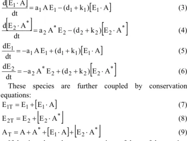
2 2 2 2 * 2 2 _{a A E (d k )E A} dt dE _{=− + + ⋅ (6)}

These species are further coupled by conservation equations:

[

E A

]

E E_1T = ₁+ ₁⋅ (7)

[

*

]

2 2 T 2 E E A E = + ⋅ (8)

[

]

[

*

]

2 1 * T A A E A E A A = + + ⋅ + ⋅ (9)

If the time-dependent concentrations of three of the species, (for example A, [E1·A], and [E2·A*]), along with the total concentrations for each component (AT, E1T, E2T) can be measured, then (1)-(9) can be used to estimate the values of the parameters of the system, namely the rate constants a, d, and k for both reactions. It is these rate constants that are the quantitative measure of interaction between the components A, E1, and E2 in this simple system. This is a difficult task for even an isolated in vitro system, and totally infeasible for a signaling intermediate within a cell. In protein kinase cascades it may be possible to determine the identity and concentration of kinase E1, but often the phosphatase E2 is undefined and assumed to be one of several nonspecific enzymes. Thus, it may be unrealistic to consider E2 or [E2·A*] as measurable quantities, and it becomes impossible to solve these equations. Furthermore, estimation of the individual rate constants may not be informative, particularly if the behavior of a network of intermediates is being investigated.

Instead of considering the dynamic behavior of this system, we consider the relationship between intermediates at steady state. In this case (1)-(6) are equal to zero, and (3)-(4) can then be rearranged to yield:

[

]

1 m 1 1 1 1 1 1 K E A k d E A a A E = + = ⋅ (10)

[

]

2 m 2 * 2 2 2 * 2 * 2 A a_dA _kE A_KE E = + = ⋅ (11)

Where Km1 and Km2 are the Michaelis constants for enzymes E1 and E2, respectively. Also, at steady state the two net reaction rates must be equal:

[

]

[

*

]

2 2 1 1 E A k E A k ⋅ = ⋅ (12)

Substituting (10)-(11) into (12) and rearranging: 1 A 1 2 m 2 2 1 m 1 1 * E K / E k K / E k A A _{= ≡α} (13) From (13), it is apparent that the ratio A*_{/A, defined as the}

activation ratio ARA, is linearly proportional to the concentration of activating enzyme E1. The unknown kinetic parameters for the enzymes, as well as (most likely unmeasurable) E2, are collected together in the activation

factor α1A_{. The activation factor represents the sensitivity of} the activation ratio for A (ARA) with respect to E1, and is therefore a quantitative measure of the potential for E1 to activate A. As k1 increases or Km1 decreases, E1 becomes a more powerful activator of A, and α1A increases. Similarly, as k2 increases or Km2 decreases, E2 is a more powerful inactivator, and therefore E1 is a weaker activator of A. Fig 2. Results for an individual cycle of Fig. 1A, A) Fraction of A activated

(A*/AT) for the simple cycle, B) Activation ratios (ARA) plotted against free

activating enzyme E1. Parameter values, all curves: k1 = 10, k2 = 10, Km2 = 1,

E2T = 1, AT = 10; Km1 = 20 (diamonds), 10 (squares), 4 (triangles), 2 (x s), 1

(stars), 0.4 (circles), 0.2 (+ s).

Simulation results for the individual cycle are shown in Fig. 2. Michaelis-Menten kinetics were assumed, and a1 was varied so as to vary Km1 100-fold without affecting k1. The fraction of A in the active form, A*_/A

T, is shown in Fig. 2A, while ARA is plotted in Fig. 2B. The curves change in shape in Fig. 2A, and do not have a simple form that can be fitted easily against E1. When the data is plotted as activation ratios in Fig. 2B, a set of lines appears and α1A can be calculated easily as the slope. Note that α1A is not necessarily constant, because the concentration of free E2 is not necessarily constant and may be indirectly influenced by E1. This is determined by the concentration and degree of saturation of enzyme E2, and will be discussed in further detail below. Nevertheless, α1A does approach a limiting value and the curves in Fig. 2B are well approximated by straight lines.

0 0.2 0.4 0.6 0.8 1 0 1 2 3 4 5 Activating Enzyme E1

Fraction Active (A*/Atot)

0 5 10 15 20 0 1 2 3 4 5 Activating Enzym e E1

Activation Ratio (ARA)

A.

In the relatively simple case of an isolated cycle, use of activation ratios yields a simple linear relationship between an activating enzyme E1 and its target A. The power of this approach becomes more apparent as complicated signaling systems are considered. This is because (13) continues to be valid when the cycle is no longer isolated, but rather embedded within a signaling network. Of particular interest are the cases of converging and diverging pathways and linear cascades, as the behavior of these two model systems can be combined to examine the effects of multiple inputs on a set of interconnected intermediates, in the absence of feedback. As will be shown below, activation ratios for a particular component within a network show different functionalities upon other components of the network, depending on how it is connected to these other intermediates. Thus, calculation of activation ratios can be used as a way to explore the structure of a signaling network.

B. Linear Cascade

A common arrangement of signaling intermediates is a linear cascade, where the activated form of one intermediate is an enzyme that catalyzes the activation of the succeeding intermediate, as shown in Fig. 1B. Following a similar analysis for each cycle in the cascade as done previously for the isolated cycle, using expressions of the form of (10)-(13), the activation ratios for the intermediates are:

1 A 1 mIA IA IA 1 m 1 1 * A A_{A k}k _EE /_/K_K E AR = = =α (14) * B A mIB IB IB 2 m * 2 * B A K / E k K / A k B B AR = = =α (15) * C B mIC IC IC 3 m * 3 * C _{k E /K} B K / B k C C AR = = =α (16)

Not surprisingly, the action of each step upon the next is the same as if the cycle were isolated, as seen above. However, when considering an indirect effect, for example E1 upon ARB, the results take a quite different form. If for simplicity enzyme-substrate complexes can be considered negligible, then A* _{+ A ≈ A}

T and B* + B ≈ BT, and it can be shown that:

1 A 1 T B A * E 1 E A B B 1 A 1 α + α α = (17)

(

BA T

)

1 A 1 1 T T C B B A A 1 * B A * T C B B A * A 1 E 1 E A B A 1 A B C C α + α + α α α = α + α α = (18)

The sensitivity of the overall cascade is a product of the sensitivities at each individual level (multistep sensitivity), as has been described previously[4, 6, 8, 34]. However, the expression for the activation ratios changes in form, from linear to hyperbolic, depending on which upstream enzyme is being considered. For example, although ARB is linear with respect to A*_{, it is hyperbolic with respect to E}

1. ARC is hyperbolic with respect both to A* _{and E}

1, but linear with respect to B*_{. This radical change in form can be readily}

visualized graphically. We can thus use this approach to suggest if a step is missing between two intermediates of interest. Note, however, it is not possible to distinguish between one or more missing steps. In this example, it is possible to know that C is indirectly downstream of E1 and A, but not by how many steps. By establishing direct links between E1 to A, A to B, and then B to C, however, the cascade structure can be realized.

The expressions in (17)-(18) arise from the assumption that enzyme-substrate complexes can be neglected in the conservation relationships for A and B. Nevertheless, the

patterns for activation ratios still hold even if these are

assumptions are relaxed. Thus, the plots for activation ratios will continue to be linear for direct effects and hyperbolic in shape for indirect effects.

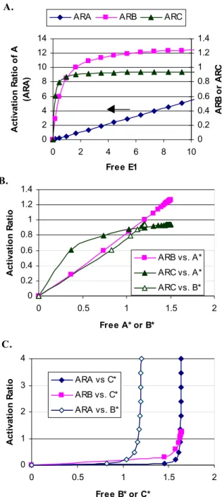
Plots of activation ratios for the model cascade of Fig. 1B are shown in Fig. 3A-C. Each step in the pathway is saturated, with AT, BT, and CT all equal to 10 and Km values in the range of 0.50-4. Thus enzyme-substrate complexes will not be negligible compared to the free species in this case. In Fig. 3A the activation ratios for each intermediate are plotted against E1. As expected, the curve for ARA is linear while the curves for ARB and ARC are hyperbolic. Similarly, in Figure 3B the plots of ARB against A* and ARC against B* are linear, while ARC against A* is hyperbolic. The activation ratio plots differ dramatically in pattern depending on whether the activating enzyme used for the abscissa is directly or indirectly activating the intermediate plotted on the ordinate.

We have thus far seen that plots of activation ratios of intermediates will be linear or hyperbolic when plotted against intermediates directly and indirectly upstream, respectively. What if we now look at downstream intermediates? In other words, what do the plots of activation ratios of intermediates against their direct and indirect targets look like? Again for simplicity, if enzyme-substrate complexes are neglected, then the following results can be obtained:

(

)

* T C T T C * * C B 1 C B C B B B B − +α α = (19)

(

)

(

)

[

]

* T C B T B A T T T C B B A * * T B A T T B A * * C B 1 A 1 C B A C B A 1 B A B A A α + α + − α α = α + − α = (20)

The activation ratios ARA and ARB in (19)-(20) take the form of an inverse hyperbola (technically, the upper left quadrant of a hyperbolic section). Thus, the activation ratio for an inverted response has a quite distinct functionality from either type of forward response. It should be further noted that the forms of (19)-(20) are the same. Therefore it is impossible to distinguish between a direct and indirect inverted response; it can only be said that the presumed target and activator are actually in reverse order. This can be seen in Fig. 3C, where ARA and ARB are plotted against B* and C*. In all cases an inverse hyperbola is seen. As above, (19)-(20)

explicitly hold only when enzyme-substrate complexes are negligible, but the forms of the equation will still be valid if this assumption is relaxed, as demonstrated in Fig. 3C.

Fig. 3. Activation ratios for the linear cascade of Fig. 1B. A) Activation ratios for cascade intermediates plotted against E1, B) ARB (closed squares)

and ARC (closed triangles) against A*, or ARC against B* (open triangles), C)

ARA against B* (open diamonds) or C* (closed diamonds) and ARB against

C* (closed squares).

In summary, comparing (15), (17), and (19) it is possible to see that the activation ratio for an intermediate (here, ARB) will be linear, hyperbolic, or inverse hyperbolic when plotted against its direct activator (A*_{), indirect upstream activator} (E1), or downstream target (C*), respectively. Activation ratios can therefore be a powerful tool to arrange intermediates in a cascade based on simultaneous measurements of activation for each component.

C. Converging Pathways

In converging pathways, two separate enzymes act independently to activate an intermediate, as shown in Fig. 1C. One example is the activation of Pbs2p by either Ssk2p/22p isoforms or Ste11p in the yeast high osmolarity (HOG) pathway[35]. In this case, either enzyme E1 or E2 can bind and activate A, although they cannot both bind A simultaneously. The activation of A therefore becomes a combination of the effects from the two enzymes, and the expression for the activation ratio becomes:

2 A 2 1 A 1 mIA IA IA 2 m 2 2 mIA IA IA 1 m 1 1 * E E K / E k K / E k K / E k K / E k A A α + α = + = (21) From (21) we see that the activation ratio for an intermediate of converging pathways is a linear combination of terms arising from (and only dependent upon) each activator. The effects of the two activating enzymes are thus completely separated. Moreover, the expression for each enzyme in (21) is the same as if E1 and E2 were acting upon unrelated substrates. Thus each enzyme is unaffected by the presence of the other. This must be the case since it is conceptually possible to separate one enzyme into two identical pools, and we would expect that the total effect of the two pools would be indistinguishable from the original state.

Since the enzyme effects are separated in (21), it is possible to calculate the activation ratio for each enzyme by varying them independently. By keeping E2 constant at any value and varying E1, it is possible to calculate α1A; α2A can be similarly determined by keeping E1 constant. These two can be compared to indicate the relative strength of the two branches on the activation of A. Varying both simultaneously will lead to an additive effect that can be predicted using the parameters calculated for each enzyme in isolation, or calculated using a multiple analysis of variance (MANOVA). Also, the presence of a second activating enzyme can be predicted since a plot of ARA against E1, for example, will not pass through the origin. Graphically, the activation ratio plots of an intermediate at a convergence point will appear as a set of parallel lines when plotted against either enzyme.

For an intermediate at a convergence point, (21) shows that the activation ratio is a linear combination of the effects from the direct activators E1 and E2. Furthermore, the expression for each term is the same as if there were no second activator. What if either E1 or E2 (or both) are not direct activators of A? In that case the term for the indirect activator changes from linear to hyperbolic in form, just as was seen in (17)-(18) for a linear cascade. Instead of a set of parallel lines, plots of activation ratios for the common target will appear as a set of hyperbolic curves when plotted against the indirect activator. It is still possible to determine that there are two activators for the intermediate, but the plots cannot be used to calculate activation ratios for the two direct activators independently.

0 1 2 3 4 0 0.5 1 1.5 2 Free B* or C* A cti va ti o n R ati o ARA vs C* ARB vs. C* ARA vs. B* 0 0.2 0.4 0.6 0.8 1 1.2 1.4 0 0.5 1 1.5 2 Free A* or B* A cti va ti o n R ati o ARB vs. A* ARC vs. A* ARC vs. B* 0 2 4 6 8 10 12 14 0 2 4 6 8 10 Free E1 A cti va ti o n R ati o of A (A R A ) 0 0.2 0.4 0.6 0.8 1 1.2 1.4 AR B o r AR C

ARA ARB ARC

C. A.

D. Diverging Pathways

A final simple signaling system to study is the case of branching pathways as shown in Fig. 1D, where one enzyme E1 activates two different targets A and B. Since there is no direct interaction between A and B we would not expect one to influence the activation of the other. We can see that this is indeed the case.

1 A 1 mIA IA IA 1 m 1 1 * E K / E k K / E k A A _{= =α (22)} 1 B 1 mIB IB IB 2 m 1 2 * E K / E k K / E k B B _{= =α (23)}

Once again, the expression for the activation ratio of each intermediate is the same as if they were isolated, and the activation factors α1A and α1B determined only from parameters arising from the interaction between E1 and A and B, respectively. The only interaction between A and B arises from sharing the activating enzyme E1. If A and B were actually different pools of the same enzyme then we would rightly expect that (22)-(23) have the same form, and the same value for α1A and α1B. Once again by neglecting enzyme-substrate complexes, it can also be shown that:

* T * B 1 A 1 * B B B A A − α α = (24) * T * A 1 B 1 * A A A B B − α α = (25)

Therefore for branching pathways, we expect that plots of activation ratios for each branch would be linear with respect to their common activator, just as if there were no other branch present. But plots of activation ratios for the two branch intermediates against each other will be inversely hyperbolic, as if each were upstream of the other. This is a quite distinct result from the case of a linear cascade seen above. In the linear cascade only one plot would be inversely hyperbolic, and the other would be linear or hyperbolic.

E. Summary: Rules for network study

Collecting these results together, it is possible to develop an algorithm for the combined analysis of a signaling network, using measurements of active and inactive amounts of the intermediates (EI* and EI). From these measurements it is possible to calculate activation ratios for each species (ARI) and plot them against the amounts of other active intermediates, EJ*. Several possibilities exist:

1) If the plot is linear, then EJ directly activates EI (EI is immediately downstream of EJ). The slope of the line is αJI. A nonzero intercept suggests the possibility of another activator for EI.

2) If the plot is hyperbolic, then EJ indirectly activates EI. One or more steps exist between EJ and EI. The cascade must be determined using direct results for other intermediates between EJ and EI.

3) If the plot is inverse hyperbolic, then either a) EI is actually upstream of EJ by one or more steps or b) EI and EJ

are on the same level of different branches from an unknown third intermediate. These two possibilities can be distinguished by considering plots of ARJ against EI* as well as ARI and ARJ against other intermediates EK*.

If there exist multiple inputs to the system, then these studies can be performed for each input individually, as well as two or more together. For intermediates at convergence points, sets of curves are expected when two inputs are both varied. As described above, sets of lines are expected for plots of ARI against a direct activator EJ, while sets of hyperbolic curves are expected for an indirect activator.

Observations regarding the shapes of curves can be determined visually, and often it will be advantageous to examine the activation ratio plots for each intermediate to gain confidence in the method and results. Nevertheless, it is possible to automate this algorithm, by performing both linear and nonlinear regression (using hyperbolic and inverse hyperbolic models) for each pair of intermediates. The model with the best least-squares error is likely to best approximate the data. In either case, the quality and quantity of the data can have a strong influence on the accuracy of analysis results. With few data points, that have high error and/or poor coverage of the range of variation for activation of the intermediates, it will be extremely difficult to determine with confidence the shape of a curve, in particular to distinguish between a line and hyperbola (direct vs. indirect activation). Thus, it will most likely be possible to develop a potential network but with few direct effects determined, and sequence determined mostly by where inverse hyperbolas can be visualized.

F. Importance of measuring free vs. total concentrations

The method of activation ratios can be quite powerful for the reconstruction of signaling networks, as illustrated using the model network above. There is an important consideration, however, which is that the analysis depends on

the measurement of free (unbound) intermediates. In other

words, it is critical to resolve between signaling intermediates in their free active and inactive forms (A* _{and A) from when} they are bound to other intermediates, including enzyme-substrate complexes (e.g. [E1·A], [E2·A*], [A*·B], etc). As an example, consider the isolated cycle of Fig. 1A. In this system there exist six species: A*_{, A, (free active and} inactive); E1, E2, (free enzyme 1 and 2); and [E1·A], [E2·A*] (enzyme-substrate complexes). At steady state (10)-(13) hold, and the activation ratio (defined as the ratio of free active to free inactive, A*_{/A) is linearly dependent upon E}

1.

If we are unable to resolve the free species from complexes, then we may only be able to measure “total” active and inactive A (AT* and AT, respectively), and total concentrations of enzymes E1T and E2T. These total concentrations are related to the components of the system in the following way:

[

E A

]

A AT = + 1⋅ (29)

[

*

]

2 * * T A E A A = + ⋅ (30)

[

E A

]

E E_1T = ₁+ ₁⋅ (31)

[

*

]

2 2 T 2 E E A E = + ⋅ (32)

Since we probably do not know Km1 and Km2, we cannot use (10)-(11) to help calculate the free species from measurements of the totals AT, AT*, E1T, E2T and (29)-(32). Thus, we will be unable to calculate or estimate the true activation ratio ARA based on “total” activation measurements. If instead of free species, the total active AT* and total inactive AT concentrations are used, the results are no longer as useful for network reconstruction. This is because: A E K A E K E k E k E K E K E k E k A A T 1 1 m * T 2 2 m T 2 2 T 1 1 1 1 m 2 2 m 2 2 1 1 T * T + + + + = + + = (33)

In (33) the ratio of “total active” AT* to “total inactive” AT is no longer linear with respect to free E1, or even to total E1T, but rather hyperbolic with respect to both E1 and E1T. Thus a direct effect, when examined using total active and inactive species, takes the same form as an indirect effect using only free species.

Results for the linear cascade are even more complicated, since AT* will now be the sum of free A* and that complexed both to the inactivase EIA and to the target B:

1 1 m 2 m mIA IA mIA IA IA 1 1 T * T E K K K B E K E k E k A A + + + = (34) * 2 m 3 m mIB IB mIB IB IB * 2 T * T A K K K C E K E k A k B B + + + = (35)

The ratios in (34)-(35) are hyperbolic with respect to the upstream activator, and the concentrations of targets (B, C) also appear. It has therefore become impossible to isolate a cycle within a cascade, or to calculate the effects of the activator alone. It can be shown that the ratio BT*/BT is still hyperbolic with respect to E1, just as for the activation ratio ARB calculated from free B* and B. Therefore, for both direct and indirect effects, a ratio of total active to total inactive concentrations for a species will take the same form. It has become impossible to distinguish between direct and indirect effects, or to calculate an activation ratio to characterize the direct interaction.

This effect is also serious in the case of converging pathways as in Fig.1C. In this case (21) becomes:

2 1 1 m 2 m 2 m I mIA IA IA 2 2 2 2 m 1 m 1 1 m I mIA IA IA 1 1 T * T E E K K K E K E k E k E K K E K E K E k E k A A + + + + + + + = (36)

The ratio of total active to total inactive is now hyperbolic with respect to both inputs, and each term in the sum contains both inputs, so the effects of the two inputs are no longer separated into different terms.

IV. DISCUSSION

Signal transduction networks can show considerable complexity, not only in the number of intermediates or interactions between these components, but also in the quantitative variability in the degree of engagement of different pathways. In the study of signaling two questions become important:

1) Which pathways are activated in response to a particular stimulus?

2) How much are these pathways activated?

The first question is qualitative in nature, but can be considered quantitative since there must be some minimum “threshold” activation for the pathway to be considered active. The answer to this question is the structure of the signaling network. The second question is entirely quantitative, asking for numbers to describe the interaction between signaling components. These numbers can then be compared when either the stimulus or the network is perturbed (for example using inhibitors); these comparisons can yield additional information about the structure, flexibility, and regulation within the network.

Previous attempts at analysis of signaling networks have generally fallen into one of two categories: dynamic (mechanistic) models or Metabolic Control Analysis (MCA) extensions. Dynamic models, which include logical and stochastic as well as deterministic models, are often based upon a specifically determined structure and assumed mechanism for each interaction. Total concentrations of species, as well as parameters for the interactions (such as kcat and Km values for enzymes) must be measured, estimated, or assumed, typically using data taken from in vitro experiments and therefore questionable in accuracy in vivo. MCA methods also depend upon a pre-existing assumed network structure. However, parameters of the analysis, such as control coefficients and elasticities, are estimated from in vivo data. The major drawback of MCA is that it depends upon the measurement of fluxes, i.e. reaction rates, as well as measurements of the intermediates[25, 27]. In metabolic pathways, these fluxes can be estimated at steady state using mass balancing and also by combination of mass spectrometry or NMR measurements with stable-isotope labeled substrates. In signaling pathways, however, these fluxes may not be actually measurable, since intermediates tend to cycle between different states, so there is no “throughput” flux that is externally observable. It may be that for this reason MCA has not been applied extensively to signaling data, in spite of excellent efforts to develop the theory.

We therefore sought to develop a method for examination of signaling networks that could be applied to a more realistic data set, and is able to answer the two questions posed above. In particular, our method can be applied to the reconstruction of the network structure, without prior assumption, and simultaneous quantitative characterization of direct effects via calculation of activation factors. If a prior network structure is available, the method can be used to validate the model and

then to assign parameter values (activation factors) to the interactions. The quality of the network reconstruction, and confidence in the proposed structure depends upon the quality and quantity of data available for analysis.

What types of measurements are necessary for this approach? It must be possible to estimate the concentrations of signaling intermediates in their various states, particularly the “free active” and “free inactive” as described previously. Since signaling intermediates generally seem to be in low abundance in cells, the method must be sensitive to low sample concentrations and selective for the component and state of interest. We believe that this capability for sensitive protein quantitation is possible using mass spectrometry (MS) as have been described recently, since MS can resolve between phosphorylated and nonphosphorylated peptides[36, 37]. By mixing the test sample with a stable isotope labeled reference sample, the relative peak area ratios can be used as a measure of protein concentration. Sample preparation will be key, since a large number of proteins applied to the MS may cause difficulty in selection of the proper peak. From a protein lysate, individual signaling intermediates can be purified somewhat using electrophoresis, chromatography, or immunoprecipitation. Note that it is important to know which intermediates are of interest, since those can be specifically purified and then quantified.

For each protein of interest in the network, both the free active and free active should be measured at several concentrations of the input stimulus. Using the analysis described above, these measurements can be used to calculate activation ratios for each intermediate and then compared against active amounts of other components. Utilization of multiple inputs to the system can be used to elucidate common pathways, as seen in the example network described above. Assuming that the range of values that each intermediate takes is sufficient to describe a hyperbola, line, or inverse hyperbola, the activation ratio plots can be used to reconstruct the network structure, and the slopes of any lines (corresponding to direct interactions) can be calculated using linear regression analysis to yield activation factors. Additional regression results, such as the confidence intervals for the parameters and correlation coefficient, can be used as a measure of the confidence in the parameter values.

The analysis described here was developed assuming steady state in the signaling system. This simplification greatly facilitates the overall analysis development, since concentrations of enzyme-substrate complexes can be written in terms of free species (e.g. E1 and A), as in (10)-(11), and individual kinetic parameters (kcat and Km) can be collected together as shown in (13). In the absence of a steady-state system, such as cells growing in a chemostat, this assumption will not be precisely valid. The transient nature of signaling pathways has been well documented; rather than achieving a steady state often components will peak in activation and relax more slowly[38]. Nevertheless, the method may still be applicable if a pseudo-steady state assumption can be made. A pseudo-steady state approximation is often made in

examination of enzyme systems, and is based on the assumption that the rate of formation of enzyme-substrate complexes is faster than the rate of decomposition. It may be possible to apply this pseudo-steady state assumption to the signaling system at each time point over the more global dynamics of the system. Further work in this area is warranted, to investigate the applicability of activation ratios to dynamic signaling systems.

V. CONCLUSION

We have developed a novel method for examination of signaling pathways based simply on understanding the nature of the interconverting cycles that are prominent in these pathways. We have shown that by considering the ratio of active to inactive forms of the intermediate, it is possible to write expressions that compress unknown kinetic parameters together. This approach yields a linear relationship between the activation ratio and the concentration of the enzyme that drives the activating reaction. The expressions stay simple when more complicated systems, such as converging pathways, linear cascades, and interconnected networks, are considered.

This method has several advantages to previously developed techniques. First, the form that plots of activation ratios take when considered against other intermediates changes depending upon the nature of the interaction between the target and activator. Activation can be distinguished as being a direct or indirect effect. By application of a simple algorithm, it is possible to reconstruct a network from measurements of activation ratios for the intermediates. Second, the simple relationships between activation ratios and concentrations of activating enzymes allow easy calculation of factors that are representative of the strength of activation and can be compared between different sets of conditions. These factors can be calculated using simple linear regression tools. Standard methods for statistical analysis can be applied to give confidence in the calculation, such as the use of a correlation coefficient to estimate the accuracy of a linear model and error analysis to estimate the precision of the calculated slope.

It becomes apparent that the quantity and type of measurements of signaling intermediates both significantly influence the analysis that is possible for these systems, and therefore the utility of these measurements. By measuring changes in the inactive as well as active form of each intermediate, activation ratios can be calculated and used to reconstruct the network and quantify the interactions between intermediates.

REFERENCES

[1]U. S. Bhalla and R. Iyengar, “Emergent properties of networks of biological signaling pathways,” Science, vol. 283, pp. 381-7, 1999. [2]G. Weng, U. S. Bhalla, and R. Iyengar, “Complexity in biological

signaling systems,” Science, vol. 284, pp. 92-6, 1999.

[3]A. Goldbeter and D. E. Koshland, Jr., “An amplified sensitivity arising from covalent modification in biological systems,” Proc Natl Acad Sci

[4]A. Goldbeter and D. E. Koshland, Jr., “Ultrasensitivity in biochemical systems controlled by covalent modification. Interplay between zero-order and multistep effects,” J Biol Chem, vol. 259, pp. 14441-7, 1984. [5]E. R. Stadtman and P. B. Chock, “Superiority of interconvertible

enzyme cascades in metabolic regulation: analysis of monocyclic systems,” Proc Natl Acad Sci U S A, vol. 74, pp. 2761-5, 1977.

[6]P. B. Chock and E. R. Stadtman, “Superiority of interconvertible enzyme cascades in metabolite regulation: analysis of multicyclic systems,” Proc Natl Acad Sci U S A, vol. 74, pp. 2766-70, 1977. [7]R. Varon and B. H. Havsteen, “Kinetics of the transient-phase and

steady-state of the monocyclic enzyme cascades,” J Theor Biol, vol. 144, pp. 397-413., 1990.

[8]J. E. Ferrell, Jr., “Tripping the switch fantastic: how a protein kinase cascade can convert graded inputs into switch-like outputs [see comments],” Trends Biochem Sci, vol. 21, pp. 460-6, 1996.

[9]D. C. LaPorte and D. E. Koshland, Jr., “Phosphorylation of isocitrate dehydrogenase as a demonstration of enhanced sensitivity in covalent regulation,” Nature, vol. 305, pp. 286-90., 1983.

[10] M. H. Meinke, J. S. Bishop, and R. D. Edstrom, “Zero-order ultrasensitivity in the regulation of glycogen phosphorylase,” Proc Natl

Acad Sci U S A, vol. 83, pp. 2865-8., 1986.

[11] M. H. Meinke and R. D. Edstrom, “Muscle glycogenolysis. Regulation of the cyclic interconversion of phosphorylase a and phosphorylase b,” J Biol Chem, vol. 266, pp. 2259-66., 1991.

[12] E. Shacter, P. B. Chock, and E. R. Stadtman, “Regulation through phosphorylation/dephosphorylation cascade systems,” J Biol Chem, vol. 259, pp. 12252-9, 1984.

[13] A. R. Asthagiri and D. A. Lauffenburger, “Bioengineering models of cell signaling,” Annual Review of Biomedical Engineering, vol. 2, pp. 31-53, 2000.

[14] F. A. Brightman and D. A. Fell, “Differential feedback regulation of the MAPK cascade underlies the quantitative differences in EGF and NGF signalling in PC12 cells,” FEBS Lett, vol. 482, pp. 169-74., 2000. [15] W. R. Burack and T. W. Sturgill, “The activating dual

phosphorylation of MAPK by MEK is nonprocessive,” Biochemistry, vol. 36, pp. 5929-33, 1997.

[16] G. C. Brown and B. N. Kholodenko, “Spatial gradients of cellular phospho-proteins,” FEBS Lett, vol. 457, pp. 452-4, 1999.

[17] J. E. Ferrell, Jr. and R. R. Bhatt, “Mechanistic studies of the dual phosphorylation of mitogen-activated protein kinase,” J Biol Chem, vol. 272, pp. 19008-16, 1997.

[18] J. E. Ferrell, Jr., “How regulated protein translocation can produce switch-like responses,” Trends Biochem Sci, vol. 23, pp. 461-5, 1998. [19] C. Y. Huang and J. E. Ferrell, Jr., “Ultrasensitivity in the

mitogen-activated protein kinase cascade,” Proc Natl Acad Sci U S A, vol. 93, pp. 10078-83, 1996.

[20] B. N. Kholodenko, O. V. Demin, G. Moehren, and J. B. Hoek, “Quantification of short term signaling by the epidermal growth factor receptor,” J Biol Chem, vol. 274, pp. 30169-81, 1999.

[21] B. N. Kholodenko, G. C. Brown, and J. B. Hoek, “Diffusion control of protein phosphorylation in signal transduction pathways,” Biochem

J, vol. 350 Pt 3, pp. 901-7., 2000.

[22] A. Levchenko, J. Bruck, and P. W. Sternberg, “Scaffold proteins may biphasically affect the levels of mitogen-activated protein kinase signaling and reduce its threshold properties,” Proc Natl Acad Sci U S

A, vol. 97, pp. 5818-23., 2000.

[23] H. Kacser and J. A. Burns, “The control of flux,” Symp Soc Exp

Biol, vol. 27, pp. 65-104, 1973.

[24] R. Heinrich and T. A. Rapoport, “A linear steady-state treatment of enzymatic chains. General properties, control and effector strength,”

Eur J Biochem, vol. 42, pp. 89-95., 1974.

[25] L. Acerenza and A. Cornish-Bowden, “Generalization of the double-modulation method for in situ determination of elasticities,”

Biochem J, vol. 327, pp. 217-24., 1997.

[26] D. A. Fell and H. M. Sauro, “Metabolic control and its analysis. Additional relationships between elasticities and control coefficients,”

Eur J Biochem, vol. 148, pp. 555-61., 1985.

[27] J. H. Hofmeyr and H. V. Westerhoff, “Building the cellular puzzle: control in multi-level reaction networks,” J Theor Biol, vol. 208, pp. 261-85., 2001.

[28] D. Kahn and H. V. Westerhoff, “Control theory of regulatory cascades,” J Theor Biol, vol. 153, pp. 255-85., 1991.

[29] B. N. Kholodenko, S. Schuster, J. Garcia, H. V. Westerhoff, and M. Cascante, “Control analysis of metabolic systems involving quasi-equilibrium reactions,” Biochim Biophys Acta, vol. 1379, pp. 337-52, 1998.

[30] S. Schuster, B. N. Kholodenko, and H. V. Westerhoff, “Cellular information transfer regarded from a stoichiometry and control analysis perspective,” Biosystems, vol. 55, pp. 73-81., 2000.

[31] J. R. Small and D. A. Fell, “Covalent modification and metabolic control analysis. Modification to the theorems and their application to metabolic systems containing covalently modifiable enzymes,” Eur J

Biochem, vol. 191, pp. 405-11, 1990.

[32] J. R. Small and H. Kacser, “Responses of metabolic systems to large changes in enzyme activities and effectors. 1. The linear treatment of unbranched chains,” Eur J Biochem, vol. 213, pp. 613-24, 1993. [33] B. N. Kholodenko, J. B. Hoek, H. V. Westerhoff, and G. C. Brown,

“Quantification of information transfer via cellular signal transduction pathways,” FEBS Lett, vol. 414, pp. 430-4, 1997. [34] J. E. Ferrell, Jr., “How responses get more switch-like as you move

down a protein kinase cascade [letter; comment],” Trends Biochem Sci, vol. 22, pp. 288-9, 1997.

[35] F. Posas and H. Saito, “Osmotic activation of the HOG MAPK pathway via Ste11p MAPKKK: scaffold role of Pbs2p MAPKK,”

Science, vol. 276, pp. 1702-5., 1997.

[36] S. P. Gygi, B. Rist, S. A. Gerber, F. Turecek, M. H. Gelb, and R. Aebersold, “Quantitative analysis of complex protein mixtures using isotope-coded affinity tags,” Nat Biotechnol, vol. 17, pp. 994-9, 1999. [37] Y. Oda, K. Huang, F. R. Cross, D. Cowburn, and B. T. Chait,

“Accurate quantitation of protein expression and site-specific phosphorylation,” Proc Natl Acad Sci U S A, vol. 96, pp. 6591-6, 1999. [38] C. J. Marshall, “Specificity of receptor tyrosine kinase signaling:

transient versus sustained extracellular signal-regulated kinase activation,” Cell, vol. 80, pp. 179-85, 1995.