Do Peers Affect Student Achievement? Evidence from Canada Using Group Size Variation

Texte intégral

(1)2012s-31. Do Peers Affect Student Achievement? Evidence from Canada Using Group Size Variation Vincent Boucher, Yann Bramoullé, Habiba Djebbari, Bernard Fortin. Série Scientifique Scientific Series. Montréal Décembre 2012. © 2012 Vincent Boucher, Yann Bramoullé, Habiba Djebbari, Bernard Fortin. Tous droits réservés. All rights reserved. Reproduction partielle permise avec citation du document source, incluant la notice ©. Short sections may be quoted without explicit permission, if full credit, including © notice, is given to the source..

(2) CIRANO Le CIRANO est un organisme sans but lucratif constitué en vertu de la Loi des compagnies du Québec. Le financement de son infrastructure et de ses activités de recherche provient des cotisations de ses organisations-membres, d’une subvention d’infrastructure du Ministère du Développement économique et régional et de la Recherche, de même que des subventions et mandats obtenus par ses équipes de recherche. CIRANO is a private non-profit organization incorporated under the Québec Companies Act. Its infrastructure and research activities are funded through fees paid by member organizations, an infrastructure grant from the Ministère du Développement économique et régional et de la Recherche, and grants and research mandates obtained by its research teams. Les partenaires du CIRANO Partenaire majeur Ministère du Développement économique, de l’Innovation et de l’Exportation Partenaires corporatifs Autorité des marchés financiers Banque de développement du Canada Banque du Canada Banque Laurentienne du Canada Banque Nationale du Canada Banque Royale du Canada Banque Scotia Bell Canada BMO Groupe financier Caisse de dépôt et placement du Québec Fédération des caisses Desjardins du Québec Financière Sun Life, Québec Gaz Métro Hydro-Québec Industrie Canada Investissements PSP Ministère des Finances du Québec Power Corporation du Canada Rio Tinto Alcan State Street Global Advisors Transat A.T. Ville de Montréal Partenaires universitaires École Polytechnique de Montréal HEC Montréal McGill University Université Concordia Université de Montréal Université de Sherbrooke Université du Québec Université du Québec à Montréal Université Laval Le CIRANO collabore avec de nombreux centres et chaires de recherche universitaires dont on peut consulter la liste sur son site web. Les cahiers de la série scientifique (CS) visent à rendre accessibles des résultats de recherche effectuée au CIRANO afin de susciter échanges et commentaires. Ces cahiers sont écrits dans le style des publications scientifiques. Les idées et les opinions émises sont sous l’unique responsabilité des auteurs et ne représentent pas nécessairement les positions du CIRANO ou de ses partenaires. This paper presents research carried out at CIRANO and aims at encouraging discussion and comment. The observations and viewpoints expressed are the sole responsibility of the authors. They do not necessarily represent positions of CIRANO or its partners.. ISSN 1198-8177. Partenaire financier.

(3) Do Peers Affect Student Achievement? Evidence from Canada Using Group Size Variation* Vincent Boucher†, Yann Bramoullé ‡, Guy Lacroix§, Bernard Fortin**. Résumé / Abstract We provide the first empirical application of a new approach proposed by Lee (2007) to estimate peer effects in a linear-in-means model when individuals interact in groups. Assuming sufficient group size variation, this approach allows to control for correlated effects at the group level and to solve the simultaneity (reflection) problem. We clarify the intuition behind identification of peer effects in the model. We investigate peer effects in student achievement in French, Science, Mathematics and History in secondary schools in the Province of Québec (Canada). We estimate the model using conditional maximum likelihood and instrumental variables methods. We find some evidence of peer effects. The endogenous peer effect is large and significant in Math but imprecisely estimated in the other subjects. Some contextual peer effects are also significant. In particular, for most subjects, the average age of peers has a negative effect on own test score. Using calibrated Monte Carlo simulations, we find that high dispersion in group sizes helps with potential issues of weak identification. Mots clés/Keywords : peer effects, student achievement, reflection problem. *. Forthcoming, Journal of Applied Econometrics. We thank Lung-fei Lee, seminar participants at University of Toronto, Northwestern University, Université de Paris 1, and the CIRANO-CIREQ Conference on the Econometrics of interactions for insightful discussions, and three anonymous referees and the co-editor Thierry Magnac for very helpful comments. We are also grateful to the Québec Ministry of Education, Recreation and Sports (MERS) for providing the data, in particular Raymond Ouellette and Jeannette Ratté for their assistance in obtaining and interpreting the data used in this study. The views expressed in this paper are solely our own and do not necessarily reflect the opinions of the MERS. We receive excellent research assistance from Steeve Marchand. Support for this work has been provided by the Canada Chair of Research in Economics of Social Policies and Human Resources, and le Fonds Québécois de Recherche sur la Socité et la Culture and le Centre Interuniversitaire sur le Risque, les Politiques économiques et l’Emploi. † Université de Montréal and CIREQ. ‡ CIRPÉE and Department of Economics, Université Laval. § CIRPÉE, IZA and Department of Economics, Université Laval. ** Corresponding author. Department of Economics, Université Laval. Email: bernard.fortin@ecn.ulaval.ca.

(4) 1. Introduction. Evaluating peer effects in academic achievement is important for parents, teachers and schools. These effects also play a prominent role in policy debates concerning ability tracking, racial integration and school vouchers (for a recent survey, see Epple and Romano 2011). However, despite a growing literature on the subject, the evidence regarding the magnitude of peer effects on student achievement is mixed (e.g., Sacerdote 2001, Hanushek et al. 2003, Stinebrickner and Stinebrickner 2006, Ammermueller and Pischke 2009). This lack of consensus partly reflects various econometric issues that any empirical study on peer effects must address. Identifying and estimating peer effects raises three basic challenges. First, the relevant peer groups must be determined. Who interacts with whom? Second, peer effects must be identified from confounding factors. Especially, spurious correlation between students’ outcomes may arise from self-selection into groups and from common unobserved shocks. Third, identifying the precise type of peer effect at work may be hard. Simultaneity, also called the reflection problem by Manski (1993), may prevent separating contextual effects, i.e., the influence of peers’ characteristics, from the endogenous effect, i.e., the influence of peers’ outcome. This issue is important since only the endogenous effect is the source of a social multiplier. Researchers have adopted various approaches to solve these three issues; we discuss the methods and results of previous studies in more detail in the next section. As will be clear, however, there is no simple methodological answer to these three challenges. In this paper, we provide, to our knowledge, the first application of a novel approach developed by Lee (2007) for identifying and estimating peer effects. In principle the approach is promising, as it allows to solve the problem of correlated effects and the reflection problem with standard observational (non-experimental) data. Moreover the exclusion restrictions imposed by the model are explicitly derived from its structural specification and provide natural instruments. The econometric model does rely on a number of crucial assumptions, however, which makes its confrontation to real data particularly important. We empirically assess the approach using original administrative data on test scores at the end of secondary school in the Canadian province of Québec. We investigate the presence of peer effects in student achievement in Mathematics, Science, French, and History. In the process, we also provide new economic insights regarding the sources of identification in the model. This matters in particular to assess its robustness to alternative (non-linear) approaches. The econometric model relies on three key assumptions. First, individuals interact in groups known to the modeler. This means that the population of students is partitioned in groups (e.g., classes, grade levels) and that students are affected by all their peers in their groups but by none outside of it. This assumption is typical in studies of academic achievement but clearly arises from data constraints. Second, each individual’s peer group is everyone in his group excluding himself. While this assumption seems innocuous and has been used in most empirical studies, it is a key source of identification in the model, as it will become clear below. In fact, it is a main source of difference between Manski’s (1993) and Lee’s models. Manski’s approach can be interpreted as one in which each individual’s peer group 1.

(5) includes himself.1 Third, individual outcome is determined by a linear-in-means model with group fixed effects. Thus, the test score of a student is affected by his characteristics and by the average test score and characteristics in his peer group. In addition, it may be affected by any kind of correlated group-level unobservable. Lee (2007) shows that peer effects are identified in such a framework when there are sufficient groups of different sizes. One important contribution of our paper is to clarify the economic intuition behind identification. Regarding the estimation of parameters, one potentially important limitation of the method, however, is that convergence in distribution of the peer effect estimates may occur at low rates when the average group size is large relative to the number of groups in the sample (Lee 2007). This is also intuitive: excluding the individual or not from his peer group does not change much when its size is relatively large. Here two remarks are in order. First, these results are to be distinguished from the idea that the group size is a factor in a school’s production function (e.g., Krueger 2003). In Lee’s model, the effects of group sizes which are separable from the peer effects are controlled for by fixed effects in the structural model. Second, Lee’s identification method differs from the variance contrast approach developed by Graham (2008). The basic idea in this approach is that peer effects will induce intra-group dependencies in behavior that introduce variance restrictions on the error terms. These restrictions are used to identify the composite (endogenous + contextual) social interaction effects under the assumption that the variance matrix parameters are independent of the reference group size. We use administrative data on academic achievement for a large sample of secondary schools in the Province of Québec obtained from the Ministry of Education, Recreation and Sports (MERS). Our dependent variables are individual scores on four standardized tests taken in June 2005 (Math, Sciences, French and History) by fourth and fifth grade secondary school students. All 4th and 5th grade students in the province must pass these tests to graduate. One advantage of these data is that all candidates in the province take the same exams, no matter their school and location. This feature effectively allows us to consider test scores as draws from a common underlying distribution. Another advantage is that our sample is representative and quite large. We have the scores of all students for a 75% random sample of Québec schools which, over the four subjects, yields 194,553 test scores for 116,534 students. In terms of interaction patterns, the structure of the data leads us to make the following natural assumption. We assume that the peer group of a student contains all other students in the same school qualified to take the same test in June 2005. In practice, a small number of students postpone test-taking to August 2005. We extend Lee’s methodology in the empirical modeling to address this issue. However, since the difference between observed group sizes and actual group sizes is small, the correction has little effect on the results. Following Lee (2007), we estimate the model in 1. More precisely, Manski studies a social interactions model which, in terms of identification, has the same properties as a model where individuals interact in groups and each individual is included in his peer group (see Bramoullé et al. 2009).. 2.

(6) two ways: through generalized instrumental variables (IV) and, under stronger parametric conditions, through conditional maximum likelihood robust to non-normal disturbances (pseudo CML). Our results are mixed though consistent with the model. We do provide evidence of some endogenous and contextual peer effects. Based on pseudo CML estimates, we find that the endogenous peer effect is positive, significant and quite high in Math (0.83). Moreover it is within the range of previous estimates (see Sacerdote 2011 for a recent survey). However, the effect is smaller and non significant in History (0.64), French (0.30), and Science ( 0.23).2 Endogenous peer effects estimates obtained from IV methods are highly imprecise with our data even in Math. The higher precision of our pseudo CML estimates is consistent with results in Lee (2007) showing that CML estimators are asymptotically more efficient than IV estimators. As regards contextual peer effects, we find evidence that some of them matter, based on both pseudo CML and IV estimators. For instance, results from pseudo CML indicate that interacting with older students (a proxy for repeaters) has a negative effect on own test score in all subjects except Math (not significant). It is remarkable that even with large average group size relative to the number of groups, we are able to identify some peer effects. However there is also much dispersion in group sizes within our samples. We suspect that this helps identification. We study this issue systematically through MonteCarlo simulations. We find that indeed increasing group size dispersion has a positive impact on the precision of estimates. The remainder of the paper is organized as follows. We discuss past research in section 2 and present our econometric model and the estimation methods in section 3. We describe our dataset in section 4. We present our empirical results in section 5 and run Monte Carlo experiments in section 6. We conclude in section 7.. 2. Previous research. In this section, we give a brief overview of the recent literature on student achievement and peer effects, and we explain how our study complements and enhances current knowledge on peer interactions in academic outcomes.3 As discussed above, measuring peer effects is complex as it raises three basic interrelated problems: the determination of reference groups, the problem of correlated effects and the reflection problem. The choice of reference groups is often severely constrained by the availability of data. In particular, there are still few databases providing information on the students’ social networks; the Add Health 2 The effect of individual characteristics, such as gender, age, and socioeconomic background, on test scores are precisely estimated by either method, and these estimates generally conform to expectations. 3 For two recent comprehensive surveys on peer effects in education, see Sacerdote (2011) and Epple and Romano (2011).. 3.

(7) dataset is an exception, see e.g. Calvo-Armengol et al. (2009) and Lin (2010).4 For this reason, many studies focus on the grade-within-school level (e.g., Hanushek et al. 2003, Angrist and Lang 2004). Other studies analyze peer effects at the classroom level (e.g., Kang 2007, Ammermueller and Pischke 2009). The administrative data we use in this study do not provide information on classes or teachers. Therefore, we assume that for each subject the relevant reference group for a student taking the test contains all other students in the same school who have completed all courses in the subject matter by June 2005. Thus, given that the reference group is likely to include students from other classes, one should probably expect peer effects to be smaller than at the classroom level.5 Two main strategies have been used to handle the problem of correlated effects. A first strategy has been to exploit data where students are randomly or quasi-randomly assigned within their groups (e.g., Sacerdote 2001, Zimmerman 2003, Kang 2007). Results on the impact of contextual effects using randomly assigned roommates as peers are usually low though significant. However, Stinebrickner and Stinebrickner (2006) have argued that these studies tend to underestimate true peer effects as the true influence of roommates is unclear. A second strategy uses observational data to estimate peer effects. This approach is usually based on two assumptions. First, fixed effects allow to take correlated effects into account. With cross section data, these effects are usually defined at a level higher than peer groups. Otherwise, peer effects are absorbed in these effects and cannot therefore be identified. For instance, Ammermueller and Pischke (2009) introduce school fixed effects to estimate peer effects at the class level for fourth grader in six European countries. Contrary to this approach, our model allows to include fixed effects at the peer group level even with cross-section data. This is so because each student within a group has his own reference group (since he is excluded from it). The second assumption is that one observes exogenous shocks to peer group composition which allow to identify a composite (endogenous + contextual) peer effect. The strategy uses either cross-section or panel data. With cross-section data, demographic variations across grades but within schools are usually exploited (see Bifulco et al. 2010). With panel data, demographic variations across cohorts but within school-grades are usually exploited (see Hanushek et al. 2003). The reflection problem is handled using two main strategies. In most papers, no solution for this difficult problem is provided. Rather, researchers estimate a reduced-form linear-in-means model, and no attempt is made to separate the contextual and endogenous peer effects. Only composite parameters are estimated (Sacerdote 2001, Ammermueller and Pischke 2009). Note however that a number of these papers (often implicitly) assume that there are no contextual effects. In this case, the composite parameter(s) allow(s) to identify the endogenous peer effect. In a second strategy, one uses instruments to obtain consistent estimates of the endogenous peer effect (e.g., Evans et al. 1992, Gaviria and Raphael 2001). The problem here is to choose suitable instruments. For instance, Rivkin (2001) 4. Bramoullé et al. (2009) determine conditions under which endogenous and contextual peer effects are identified when students interact through a social network known by the modeler and when correlated effects are fixed within subnetworks. See also section 3.4.2. in this paper. 5 In fact, at the end of secondary level, classes and teachers are usually different depending on the subject matter taught.. 4.

(8) argues that the use of metropolitan-wide aggregate variables as instruments in the Evans et al. (1992) study exacerbates the biases in peer effect estimates. In our paper, we provide some results based on instrumental methods. However, our instruments are naturally derived from the structure of the model. In short, various strategies have been proposed to address the three basic issues that occur in the estimation of peer effects. But most rely on strong assumptions that are difficult to motivate and may not hold in practice. Some of them require panel data while others rely on experiments that randomly allocate students within their peer group. This makes the results in Lee (2007) particularly interesting, as they show that both endogenous and contextual peer effects may be fully identified even with observational data in cross-section.. 3 3.1. Econometric model and estimation methods Econometric model. We review and adapt the structural model suggested by Lee in the context of our application. Lee’s model builds on and extends the standard linear-in-means model of peer effects (Moffitt 2001) to groups with various sizes. The set of students {i = 1, ...M } is supposed to be partionned into groups of peers indexed by r = 1, ..., R. Let Mr be the rth group of peers, of size mr . All students in the same group have the same number of peers since they interact with all others in the group. We assume that student i who belongs to group r is excluded from his own reference group. Let Mri be student i’s group of peers, of size mr 1. A peer is any fellow student whose academic performance and personal characteristics may affect i’s performance. Let yri be the test score obtained by student i. Let xri be a 1 ⇥ K vector of characteristics of i and Xr be the mr ⇥ K matrix of individual characteristics. For expository purposes, the model is first presented with a unique characteristic (K = 1), defined by his family socio-economic background. Another departure from the linear-in-means model is the inclusion of a term ↵r that captures all group invariant unobserved variables (e.g., same learning environment, similar preferences of school or motivation towards education). The error term ✏ri reflects other unobservable characteristics associated with i. We do not change any other assumption of the linear-in-means model. In particular, we assume that a student’s performance to the standardized test may be affected by the average performance in his group of reference, by his family socioeconomic background, and by the average socioeconomic background in his group. Formally, the basic structural equation is given by:. yri = ↵r +. P. j2Mri. yrj. mr. 1. + xri +. P. j2Mri. xrj. mr. 1. + ✏ri ,. E(✏ri | Xr ,mr , ↵r ) =0,. (1). where captures the endogenous effect, the individual effect and the contextual effect. Observe that eq. (1) can be derived from the first-order conditions of a choice-theoretic non-cooperative (Nash) 5.

(9) model where each student’s performance is obtained from the maximisation of his quadratic utility function which depends on his individual characteristics, his performance and his reference group’s mean performance and mean characteristics. Importantly, we assume strict exogeneity of mr and {xri : i = 1, ..., mr } conditional on the unobserved effect ↵r , i.e., E(✏ri | Xr ,mr , ↵r ) =0. This exogeneity assumption can notably accommodate situations where peer group size is endogenous. Suppose that, everything else equal, brighter students attend smaller schools, i.e., schools where the cohort of students eligible to take the provincewide test in the subject matter (our peer groups) is small. In this case, peer group size mr may well depend on unobserved common characteristics of the student’s group, ↵r : E(↵r | Xr , mr ) 6=0. Our model allows for this type of correlation. However, conditional on these common characteristics, peer group size mr is assumed to be independent of the student’s idiosyncratic unobserved characteristics: E(✏ri | Xr , mr , ↵r ) =0. We maintain this assumption throughout our analysis. To eliminate group-invariant correlated effects, we next apply a within transformation to eq. ( 1). In particular, as we noted above, when the effect of group size is separable from peer and individual effects, it is captured by ↵r . The model can address the problem of selection or endogenous peer group formation. For instance, school choice may depend on some unobserved factors specific to a school ( e.g., reputation, unobserved quality) and determine the type of students who are attracted by these schools. The advantage of the within transformation is that we compare students of the same type. This transformation also allows to control for common environment effects. Resources available at the school level (e.g., teaching, physical infrastructure) may affect the performance of all the students. Again, by comparing students within the same school, we can abstract from these effects. The within reduced form equation for students in the rth group can be written as: yri. y¯r =. mr 1. 1+. (xri. x ¯r ) +. mr 1. 1 1+. ("ri. "¯r ). (2). mr 1. where means y¯r , x ¯r and ✏¯r are computed over all students in the group. Now assume that + 6= 0. Only one composite parameter can be recovered from the reduced form for each group size mr . At least three sizes are thus necessary to identify the three structural parameters , and .6. 3.2. Interpretation of identification. The fact that the parameters of the structural within eq.(2) may be fully identified is quite surprising, and deserves some elaboration. Indeed, under the alternative assumption that means are inclusive, that is, i 2 Mri , peers are the same for everyone in a group Mri = Mr , and peer effects cannot be separated out from group fixed effects. So somehow assuming that the individual is excluded from his own peer group allows to solve two difficult identification problems: distinguishing true peer effects 6. It is easy to show that when. +. = 0, only. is identified.. 6.

(10) from correlated effects and further distinguishing endogenous from contextual peer effects. Intuitively, where does identification come from? Suppose first that the endogenous effect is absent = 0. Note that each individual has different peers: i 6= k implies that Mri 6= Mrk . A first key observation is that, within a group, individual P attributes xi are perfectly negatively correlated with mean peer attributes ( j2Mri xj )/(mr 1).7 Thus, students with an ability above average necessarily have peers with a mean ability below average, and vice versa. If the individual and the contextual effects and are positive, this negative correlation tends to reduce the dispersion in outcomes. In such a group setting, peer effects lower the difference in achievement between high and low ability students.8 Formally, the impact of the difference in attributes on the difference in outcomes changes from to /(mr 1) when introducing peer effects [see eq. (2)]. So variations in group sizes can be used to identify contextual peer effects. The second key observation is that this reduction is stronger in smaller groups. The variance in mean peer attributes is simply higher in smaller groups, reflecting the relatively larger effect of excluding one individual from the mean. And as group size increases, mean peer attributes converge to the group mean, and peer effects have increasingly less bite on how differences in covariates affect differences in outcomes. Next, consider the reflection problem. Observe that outcomes are subject to a similar negative correlation: within a group, students with grades above average necessarily have peers with grades below average. So if > 0, endogenous peer effects lead to a further reduction in outcome dispersion. However, simultaneity now implies that this decrease in impact is non-linear in the peer coefficient: from /(mr 1) to ( /(mr 1))/(1 + /(mr 1)) [see eq. (2)]. The difference in the shapes of impact reduction can then be used to identify endogenous from contextual peer effects. Finally, this understanding is useful to assess the robustness of the identification strategy to changes in the econometric model. In particular, it is easy to see that if xi < xk then the distribution of attributes in i’s peer group Mri first-order stochastically dominates the distribution in Mrk . So identification is likely to hold, in general, if we replaced the mean in equation (1) by the median, the variance, or many other moments of the distribution.9. 3.3. Treatment of missing values. One problem we face in our sample is that we do not always observe the scores of all students within a group. For instance, some students may postpone test-taking to the next session due to illness. We next extend our model to allow for this possibility. Our setting is one where the total number of students (including those who postpone test-taking) in each group is known, but we only observe the test scores P P P P To see this, observe that j2Mri xj = ( j2Mr xj ) xi . So if xi < xk then mr1 1 j2Mri xj > mr1 1 j2Mrk xj . 8 In contrast if > 0 and < 0, this negative correlation helps amplify the dispersion in outcomes. 9 Of course, one has to address a basic modeling question first, that is, whether the implied model is coherent. A model has this property when a specific nonlinear structure generates a unique solution for outcomes. 7. 7.

(11) of subsamples Nr of size nr of each group Mr , with nr  mr and. R P. nr = N . We assume that a. r=1. student’s decision to postpone exam-taking is random or depends on the observable strictly exogenous variables, conditional on the fixed group effect. We show how to adapt Lee’s analysis to this more general setting. Let Lr be the complement of Nr , i.e. , Lr = Mr Nr .10 The structural equation becomes: P P j2Nri yrj j2Nri xrj yri = ↵ er + + xri + + ✏ri , E(✏ri | Xr ,mr , ↵r ) = 0, (3) mr 1 mr 1. where i now P denotes an observed individual in the sample (but not any one in the rth group) and P j2Lr yrj j2Lr xrj ↵ e r = ↵r + + is the new group fixed effect. Under our assumptions, estimators mr 1 mr 1 are consistent, even if we do not observe test scores for all students in each group. Moreover, effects stemming from unobserved individuals are the same for all the individuals observed in the sample from the rth group. They are therefore picked up by the group fixed effect. Using the within transformation, one obtains the same equation as (2) but where means y¯r , x ¯r and ✏¯r are computed only over all observed students in the group.. 3.4. Estimation methods. 3.4.1. CML Estimator. We consider estimation under both pseudo Conditional Maximum Likelihood (or CML) and Instrumental Variables (or IV) identification conditions. To present pseudo CML and IV estimators, it is easier to express eq. (3) in matrix notations. We now allow for any number of characteristics, so that is a K ⇥ 1 vector of individual effects and a K ⇥ 1 vector of contextual ones. Recall that in this setting, students are affected by all others in their group and by none outside of it. This means that the observed social interactions can be modelled as a N ⇥ N block-diagonal matrix G = Diag(G1 , ..., GR ), such that for all r, Gr is comprised of 0 elements grij = mr1 1 if i 6= j and grii = 0. In other terms, Gr = mr1 1 (◆nr ◆nr Inr ), where ◆nr is a nr ⇥ 1 vector of ones and Inr the identity matrix of dimension nr . Eq. (3) can be re-written in matrix form as follows: y r = ◆ nr ↵ e r + Gr y r + X r + Gr X r + ✏ r , (4) where E(✏r | Xr , Gr , ↵ er )=0. 0 Applying the operator matrix Jr = Inr n1r ◆nr ◆nr allows us to obtain deviations with respect to the mean for the observed group members. Pre-multiplying eq. (4) by Jr eliminates the group fixed effect and yields : J r y r = J r Gr y r + J r X r + J r G r X r + J r ✏ r (5) 10. If Nri denotes the group of peers of student i, we also have Lr = Mri. 8. Nri ..

(12) 1 m r 1 Jr .. Elementary linear algebra tells us that Jr Gr =. Letting Jr Ar = A⇤r , we obtain. mr 1 + (mr 1) yr⇤ = X⇤r mr 1 mr 1. + ✏⇤r. which is equivalent to eq. (2). To derive the pseudo CML estimator, we assume (possibly wrongly) that the ✏ir ’s are i.i.d. N(0, 2 ). It follows that, given Xr , mr , and nr , the pseudo density of yr⇤ is a multivariate normal distribution r 1) r 1 with mean X⇤r (m and variance ( mm )2 Jr .11 The pseudo log likelihood function to be mr 1+ r 1+ maximized can then be expressed as follows: ln L = c +. R X. (nr. r=1 R ✓ X. 1 2. 2. r=1. 1) ln (mr. 1+ ). mr 1 + yr⇤ mr 1. N. R. ln. 2. (mr X⇤r. 1). mr. 1. 2. ◆0 ✓. mr 1 + yr⇤ mr 1. (mr X⇤r. mr. 1) 1. where c is a constant. This log likelihood function excludes any fixed effects. It is a conditional log likelihood function as it is conditional on the sufficient statistics yr , (as well as on the Xr ’s, the mr ’s, and the nr ’s), for r = 1, ...R. Under the assumption that the ✏ir ’s are correctly specified and i.i.d. N(0, 2 ), Lee (2007) shows that the CML estimators of , , and are consistent and asymptotically efficient under regularity conditions and provided there is sufficient variation in group sizes. Even if the assumed density of yr⇤ is misspecified, the pseudo CML estimator is consistent provided that the conditional mean of the yr⇤ ’s is correctly specified. This is the case since the normal density belongs to the Linear Exponential Family (see Gourieroux et al. 1984). Of course, the estimator is no longer asymptotically efficient. Moreover, one has to compute the robust covariance matrix using the sandwich formula J 1 IJ 1 , where J is minus the expectation of the Hessian matrix and I the expectation of the outer-product-of-the-gradient matrix. A further advantage of this computation is that it allows us to see whether an apparent precision of CML estimators is driven by the normality assumption used in Lee (2007). 3.4.2. 2SLS and Generalized 2SLS estimators. Alternatively, the structural equation (4) can be estimated by instrumental (IV) methods. To see how the methods work, define a N ⇥ N block-diagonal matrix J = Diag(J1 , ..., JR ). Concatenating eq. (5) over all groups yields: Jy = JGy + JX + JGX + J✏. (6) where y (resp. X) is obtained by stacking the vectors yr (resp. the matrices Xr ), for r = 1, ..., R. 11. Note that only nr. 1 elements of ✏⇤r are linearly independent.. 9. ◆. ,.

(13) The reduced form of the model is: Jy = (I. G). 1. (JX + JGX ) + (I. G). 1. J✏.. (7). Identification can be given a natural interpretation in terms of instrumental variables. If i 2 / Mri and there are at least three different group sizes, E[JGy|X, G] is not perfectly collinear to (JX, JGX) and the model is identified [see Bramoullé et al. (2009) for more details]. Moreover JG2 X can be used as a matrix of valid instruments for JGy.12 One advantage of an IV approach over pseudo CML is that it requires less structure. Specifically, we do not assume that the specified density function of the yr ’s, potentially partially misspecified, is normal. Also we do not use the structure on the error terms for identification purpose. Thus, identification in this case is semi-parametric, or “distribution-free”. Of course, this comes at a price: the IV estimator is asymptotically less efficient than the pseudo CML, since the latter imposes more structure on the distribution of error terms. In addition, we can derive a Generalized IV estimator as proposed in Kelejian and Prucha (1998), and discussed in Lee (2007). Assuming homoskedasticity, it yields an asymptotically optimal (best) IV estimator and reduces to a two-step estimation method in our case. More precisely, our first step consists in estimating a 2SLS as described above, by using as instruments S = (JX, JGX, JG2 ). The b = (JGy, d JX, JGX), second step consists in estimating a G2SLS estimator using as instruments Z d is computed from the reduced form ( 7) premultiplied by G and using the first-step estiwhere JGy mates.. 4. Data. We gathered for this analysis original data from the Québec Government MERS. These administrative data provide detailed information on individual scores on standardized tests taken in June 2005 on four subjects (Math, Sciences, French and History) by fourth and fifth grade secondary school students. They also include information on the age, gender, language spoken at home and socioeconomic status of students. Sampling has been done in two steps. The population of interest is the set of all fourth and fifth grade secondary school students who are candidates to the MERS examinations in June 2005. This population is comprised of 152,580 students in total. In the first step, a 75% random sample of secondary schools offering fourth and fifth grade classes in the 2004-2005 school year have been selected. In the second step, all fourth and fifth grade students in these schools have been included. Overall, we have 194,553 individual test scores for 116,534 students.13 12. In fact, Jr Gr = mr1 1 Jr and Jr G2r = (mr1 1)2 Jr , hence instruments are built here by premultiplying characteristics (in deviation) by group-dependent weights and by stacking them across groups. 13 There are more individual test scores than students as some students take test in more than one subject matter.. 10.

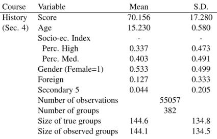
(14) There are many advantages to the use of our data. First, all 4th and 5th grade students must take tests on these four subjects to qualify for secondary school graduation. This means that our results do not pertain to a selected sample of schools. In particular, both public and private school students have to take these tests. Another advantage is that the tests are standardized, i.e., designed and applied uniformly within the province of Québec. We use test results gathered by the MERS, so there is less scope for measurement error with these data than with survey data on grades. Finally, although survey data may have provided information on a larger set of covariates, sample sizes in our study are larger than in typical school surveys. Given the lack of information on the structure of relevant social interactions, we assume that the peer group for a student taking a test is comprised of all other students in the same school who are qualified to take the test in June 2005. Two test sessions are offered for those who completed coursework in the Spring semester. We thus consider as belonging to the same group all those who belong to the same school and who take a subject test in one of the two consecutive sessions of June and August 2005. We know the number of students in each of these groups. But we only observe test scores for the set of students who took the test in June. Therefore we do not always observe the scores of all students within a group. We offered a correction for this problem in our discussion of the econometric model, and our empirical results below incorporate this correction. In any case an overwhelming majority of the students do take the tests in June, so the correction has little effect on the results. We use for this study French, History, Science and Math test results as reported in the MERS administrative data. Students in a regular track take History and Science tests in Secondary 4. The French test is commonly taken in Secondary 5. Finally, we focus on students who take the Math test in Secondary 5 (Math 514). This completes their mathematical training for secondary school. Note that the MERS administers a unique test to all secondary school students in French, History and Science. In contrast, it administers different tests in Math, depending on academic options chosen early on by the students. We report here results for students following the regular mathematical training (Math 514). We focus on this test in our analysis. We provide descriptive statistics in Table 1. For each subject, the dependent variable in our econometric model is the test score obtained in the provincial standardized test. The average score is between 70% and 75% in French, Science and History tests. It is lower and about 62% in Math. In samples for which the regular track for the test is Secondary 5 (resp. Secondary 4), the average age of students is close to 16 (resp. 15). Most students taking French and Math (98% and 96%) are enrolled in Secondary 5. Most of those taking Science and History are enrolled in Secondary 4 (92% and 96%). Between 52% and 55% of students are female, and between 11% and 13% of students speak a language at home which is different from the language of instruction (Foreign variable).14 Between 30% and 34% of students come from a relatively high socioeconomic background and between 40% and 42% 14. The language of instruction is French in most schools, and English otherwise.. 11.

(15) from a medium one. We use an index of socio-economic status provided by the MERS. This index is computed from data from the 2001 census. It uses information on the level of education of the mother (a weight of 2/3) and the job status of parents (weight of 1/3). Low socio-economic status corresponds to the three lowest deciles of the index (high socio-economic status to the three highest deciles). We observe test scores and characteristics of students taking the same test in June 2005. Sample sizes are 41, 778 for French, 54, 981 for Science, 15, 771 for Math, and 55, 057 for History. We also observe the number of students who completed coursework but postpone test-taking to August 2005. There are 118 students postponing French, 186 postponing History, 195 postponing Science, and 160 postponing Math. We observe between 314 and 382 peer groups depending on the subject matter considered. The average group size is between 50 (Math) and 146 (Science). The ratio between the number of groups and the average group size varies between 2.36 (French) and 7.23 (Math). These numbers are relatively small, which suggests that our estimates could be subject to weak identification problems. The group size standard deviation is quite large, however, varying between 50 (in Math) and about 135 (in Science and History). We expect such dispersion in group sizes to help identification. We analyze these issues in more details in Section 6.. 5 5.1. Empirical Results CML and pseudo CML estimates. Table 2 reports the results of maximum likelihood estimation with unrobust (CML) and robust (pseudo CML) standard errors. The model estimated is the linear-in-means model with group fixed effects, individual impacts, and endogenous and contextual peer effects. We find that the estimated endogenous peer effect lies between 0.24 and 0.83. Using unrobust standard errors (in brackets), the endogenous effect is significantly different from zero and positive for Math ( b = 0.82), and History ( b = 0.65). It is not significant for French ( b = 0.33) and for Science ( b = 0.23). Based on robust standard errors, it is no longer significant for History (p-value= 10,82%) but still significant for Math. One thus concludes that regarding this peer effect, inference appears to be driven by normality for one subject (History). In general standard errors are larger using pseudo CML than CML, but their differences are not so important. Two reasons may explain why the endogenous peer effects in Math is significant in our sample. First, the standard error of the estimates is smaller in Math than in other subjects. This is consistent with the fact that the average group size relative to the number of groups is close to three times smaller in Math than in other subjects. Second, our endogenous effect estimate is much larger in Math (0.82). How does this result compare with other studies? Sacerdote (2011) has recently provided a survey of studies of endogenous peer effects in test scores for primary and secondary schools based on linearin-means models (see his Table 4.2.). Interestingly, in most reported studies (5 over 6) which analyze achievement in both Math and Reading, the endogenous peer effect is larger in Math. In addition, this 12.

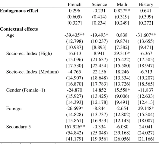
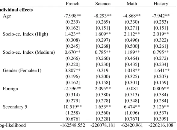
(16) effect is often very high and exceeds the value we have estimated. Thus Hoxby (2000) reports a 1.7 to 6.8-point increase in own score in relation with a 1-point increase in mean score of peers in some specifications. Betts and Zau (2004) show a 1.9-point increase in association with a 1-point increase in mean math score of peers. On the other hand, Hanushek et al. (2003) obtain a Math peer effect of 0.4.15 So our estimate lies on the average to high side of the range of previous estimates. Observe finally that our results in Math are larger than those usually obtained in studies based on randomized experiments (e.g., Sacerdote 2001, Zimmerman 2003). One possible explanation is that peers used in these papers are often people from the same dorm. These individuals do not necessary represent those who exercise significant influence on students’ scholar achievement. The relatively large endogenous peer effect in Math may reflect the fact that mathematics provide more opportunities for interactions among students. And, probably more than in other subjects, it may also reflect general effects such as disruption. For instance, it is likely that success in Math requires much concentration in class from the average student. Now suppose that there is a student (with low grade in Math) in class who is characterized by his propensity to disrupt learning by bad behavior or asking poor questions. His behavior may have large negative effects on his peers’ scholar achievement (e.g., see Lazear 2001) and thus generates strong endogenous peer effects. Regarding the individual characteristics, most of them have a significant effect on test scores, and the signs of these effects essentially conform to expectations. All test scores decrease significantly with age. Since older students have often repeated a grade, being younger is a natural proxy for ability. Test scores are significantly higher for female students than for male students, except for History where male students perform significantly better than female students. This is broadly consistent with results from previous studies. For instance, results from the 2000 Program for International Student Assessment (PISA) show that Québec female students perform better than males on reading literacy tests but that the differences in performance on mathematics and science tests are smaller and not significant (see Québec Government 2001). Similarly, in our analysis, the difference in performance is quantitatively large in French but much smaller in the other disciplines. The performance of foreign students is, non surprisingly, significantly lower than for non-foreign students on the French test, but higher for Science and History and not significantly different for Math. Secondary 5 students tend to perform significantly better on all tests than Secondary 4 students, which reflects the positive impact of an additional year of schooling on test scores. Finally, students from a higher socioeconomic category perform significantly better in all tests. As far as contextual variables are concerned, a few of them have a significant impact on student performance. Average age of other students has a negative and significant effect on all test scores except Math where it is positive but not significant. These results also conform our expectations. When the number of repeaters rises (as reflected by an increase in mean age of our peers at a given 15. Kang (2007, p. 475) also provide a survey of endogenous peer effects in achievement in mathematics which is broadly consistent with results reported in Sacerdote (2011).. 13.

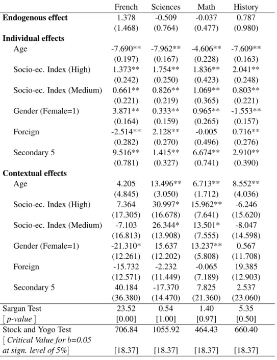
(17) grade level), this will tend to reduce own test score. Proportion of other students enrolled in Secondary 5 have a large positive and significant effect on own score in French. Peers’ socioeconomic background has little effect on own schooling performance. The proportion of female students among peers has a positive and significant effect in Math. When significant, the magnitude of contextual effects is always larger than the magnitude of individual effects. This is not surprising as it captures the effect of a unit change in the characteristic of every other student in the group.16. 5.2. Reflection problem. One way of addressing the simultaneity problem without exploiting group size variations is to exclude at least one contextual variable from the outcome equation and to use it as an instrument for average test score. We estimate a model similar to the one presented in Table 2 but excluding contextual effects that are not individually significant in the pseudo CML specification (i.e., for which the null that = 0 is not rejected); see Table 1 of the Supplementary Data Appendix.17 Using likelihood ratio tests, we reject the null that these ’s are jointly equal to zero for French but not for the other subjects. This suggests that the exclusion restrictions may be valid for these latter samples. Therefore, the pseudo CML estimators provided in Table 1 of the Supplementary Appendix should be consistent and asymptotically more efficient than those provided in Table 2 for the Science, Math and History tests. Results however appear to be robust to these new specifications. Observe finally that we could not have known this a priori without an estimation of the full model. Overall, this shows the interest of Lee’s solution to the reflection problem. Estimating a model with both endogenous and contextual peer effects is needed to recover the different types of peer effects at work.. 5.3. 2SLS and G2SLS estimates. Tables 3, and Table 2 of the Supplementary Appendix provide the 2SLS and G2SLS estimation results of the linear-in-means model of peer effects with group fixed effects, individual impacts, and endogenous and contextual peer effects. In contrast to the CML and pseudo CML estimates of Table 2, none of the endogenous effects is statistically significant. This is consistent with Lee’s (2007, p. 345) result that the asymptotic efficiency of IV estimators is smaller than that of the CML. Estimated individual effects are quite similar to the corresponding CML estimates. Some contextual effects are similar while others are different. For instance, the proportion of other students in Secondary 5 still has a large and positive effect on own French score as well as no significant effects for the other subjects. In contrast, average age among peers now has a positive and significant effect on own score for most subjects, rather than a negative one. This could be explained by differences in small sample properties of both methods, possibly aggravated by the imprecision in the estimation of the endogenous peer effect. 16 We have also estimate a second-order pseudo CML in which restrictions are directly incorporated in the variance term and estimated. Results are quite similar with those presented in Table 2. 17 This Appendix is available on the Journal of Applied Econometrics’ website.. 14.

(18) Table 3 also reports two standard test results giving information on instrumental variables properties. We first look at Sargan tests on the validity of instruments and the over-identification restrictions of the model. We do not reject the null for Science, Math and History, but we reject it for French. While this may indicate a problem of model specification in this last case, one must be cautious in interpreting the test given the likely low convergence of peer effects IV estimates. We then compute Stock and Yogo test statistics on weak identification. Based on the definition that a group of instruments is weak when the bias of the IV estimator relative to the bias of ordinary least squares exceeds a certain threshold b, say 5%, one rejects the null that the instruments are weak for all subject matters. Finally, Hausman tests have been performed to test the equality of pseudo CML and G2SLS estimators. Under the null, both of these estimators are consistent, but pseudo CML estimators are asymptotically more efficient; under the alternative, G2SLS estimators are consistent whereas pseudo CML estimators are not. For each subject, we could not reject the null. This suggests the absence of specification errors in the model.. 6. Monte Carlo simulations. In this section, we study through simulations the effect of group sizes and their distribution on the precision and bias of our estimates. Lee (2007) shows that the CML and IV estimators may converge in distribution at low rates when the ratio between the the number of groups and the average group size is small. Since this ratio varies between 2.36 and 7.23 in our samples, a problem of weak identification could in principle emerge. However, the standard deviation of the distribution of group sizes is also relatively large (see Table 1), and we suspect that this may help identification. To study these issues, we realize two simulation exercises. First, we vary group sizes in a systematic manner and study how this affects the bias and precision of estimators. To focus on the approach which provides the most reasonable findings in our empirical analysis, we report results on the model using CML.18 We look at uniform distributions, vary the size of the distribution’s support and partly calibrate simulation parameters on our data. Second, we look at bias and precision of estimates for fully calibrated simulations, when group sizes are exactly the same as in the data. Overall, while our analysis confirms Lee’s earlier results, we also find a strong positive impact of the dispersion in group sizes on the strength of identification. Especially, conditional maximum likelihood performs well on fully calibrated simulations. This suggests that the bias due to small sample issues is likely low in the results presented in Table 2. For each simulation exercise, we keep the number of observations fixed around 42, 000, and run 1, 000 replications. We first consider average sizes of 10, 20, 40, 80 and 120. We pick group sizes from the following intervals with decreasing length: 18 In an earlier version of the paper, we also provided results for IV estimates. Basically, the results are qualitatively the same for IV as those for CML but, as expected, the magnitude of the bias and the loss in precision are always larger for IV than for CML.. 15.

(19) • Average size of 10 : [3, 17], [5, 15], [7, 13] and [9, 11], • Average size of 20 : [3, 37], [8, 32], [13, 27] and [18, 22], • Average size of 40 : [3, 77], [12, 68], [21, 59], [30, 50] and [39, 41], • Average size of 80 : [3, 157], [18, 142], [33, 127], [48, 112] and [63, 97], • Average size of 120 : [3, 237], [28, 212], [53, 187], [78, 162] and [103, 137]. For each of the intervals described above, we proceed in the following manner: - pick a group size from a uniform distribution for which the support is defined by the minimum and maximum value of the interval; - truncate this value by eliminating its decimal portion; - repeat step 1 and 2 as long as the total number of observations is below or equal to 42, 000. To reduce computing time, we assume that students have the same characteristics except for age and gender. We assume that age follows a normal distribution and gender follows a Bernoulli distribution. We calibrate the moments of these distributions on the sample of students taking the French test: average age is 16, variance of age is 0.25, and proportion of girls is 0.55. Values of the structural parameters , and are set close to the estimated coefficients for the French test: = 0.35, age = 8, gender = 3.8, age = 40, gender = 25. We assume that the values of ✏ in the structural equation are drawn randomly from a normal distribution with mean zero and variance 2 = 1. We generate the endogenous variable y from the reducedform equation in deviation form. Looking at Table 4, we first compare simulation results across average group sizes and then we examine how estimators perform for a given average group size as dispersion in group size decreases. Separate horizontal panels in Table 4 pertain to different values of average group size. We report the average estimated coefficient and standard error for the endogenous effect (first vertical panel), the contextual effect associated with age (second vertical panel) and the contextual effect associated with gender (third vertical panel). We find that even for the largest average group size (i.e., 120), CML may perform well in terms of bias and precision (first line in the last horizontal panel of Table 4). The biases of CML get in general larger as average group size increases. The CML estimate of the endogenous effect attains a plateau at the value 1. This is consistent with the fact that the CML estimator tends towards the naive OLS estimator as group sizes become larger. In general, peer effects are also less precisely estimated in large groups than in small groups. Our main new result concerns the effect of group size dispersion. When we fix the value of the average group size and reduce the length of the interval from which group sizes are picked, we find that the bias of CML typically increases while the precision typically decreases. In Table 4, this amounts to 16.

(20) looking at each horizontal panel separately. Observe however that since we roughly pick group sizes from a uniform distribution holding average group size fixed, reducing the interval’s length affects the two parameters of the size distribution (i.e., the minimum and maximum value of its support) and a number of its moments. In particular, this leads to a reduction in variance and to an increase in the size of the smallest groups. In general, both the variance and the size of smallest groups may matter and the strength of identification may depend on the size distribution in complex ways. We leave a deeper investigation of this issue to future research. We next fully calibrate the simulations’ parameters on the data. We use observed group sizes in the French sample, calibrate the model parameters { , age , gender , age , gender } and moments of the explanatory variables as previously, and set the variance of the error term in the structural equation equal to the estimated variance in the French sample (ˆ 2 = 154.7). Simulation results which now report both CML and IV estimates are reported in Table 5. The CML estimator has small bias and standard error, while the IV estimator is not precisely estimated and the bias is large. These results confirm for CML what we obtained from picking group sizes at random; they show that dispersion in group sizes help identification. Besides, this suggests that small sample bias may be relatively high in the IV estimates of Tables 3, and of Table 2 of the Supplementary Appendix but relatively low for the CML estimates of Table 2.. 7. Conclusion. This paper provides an analysis of social interactions in scholar achievement when students interact through groups. Based on a linear-in-means approach with group fixed effects (Lee 2007), we make two main contributions regarding the identification and estimation of peer effects. First, we provide a new intuition for identification. We show that full identification of the model relies on three key properties: (1) Since the individual is excluded from his peer group, above average students have below average peers (with respect to any attribute). Therefore, when individual and peer effects are positive, peer effects then tend to reduce the dispersion in outcomes. (2) This reduction is stronger in smaller groups, reflecting the larger effect of excluding one individual from the mean. (3) Contextual and endogenous peer effects generate reductions of different shapes, which allow to identify both of them. Second, as regards the estimation of peer effects, the model is applied to original administrative data providing individual scores on standardized tests taken in June 2005 in four subjects by fourth and fifth grade secondary school students in the Province of Québec (Canada). Based on a pseudo conditional maximum likelihood approach, our results indicate that students significantly benefit from their peers’ higher test scores in Math but not in other subjects such as Science, History and French. Two reasons may explain these results. First, this is likely to reflect the fact that Math provides more opportunities for interactions among students. Second, in our sample, the average group size (relative to the number of groups) is close to three times smaller in Math that in other subjects. As suggested by 17.

(21) Lee (2007), accurate estimation of peer effects requires relatively small groups. This is also confirmed by our Monte Carlo simulations. These results should be warning applied researchers in the future against using data in which the size of groups is too large. Besides, our simulations indicate that, for a given average group size, increasing group size dispersion improves the precision of peer effects estimates. In fact, our results suggest that, conditional on estimating on the whole sample, even data on larger groups may provide useful information for estimation purposes. The basic intuition is that data on very large groups can be used to provide more precise individual effects estimators. In turn, this indirectly provides more efficient estimates of the peer effects from data on smaller groups. So, future estimations of Lee’s model may benefit from data with relatively small average group size but relatively large group size dispersion, including both small and large groups. In terms of public policy, the fact that the endogenous peer effects appear to be very large in Math suggests that a reform that improves the amount and quality of Math learning is likely to yield very high returns in terms of scholar achievement. This is so since such a reform will not only have direct effects on student performance in Math but also strong indirect effects through the additional external benefits generated by the social multiplier. Remarkably, our analysis also shows that the indirect peer effects of the reform will reduce performance inequalities in Math across students. This is the case because low-ability students have better peers (since their peers exclude them) and high-ability students have worse peers (for the same reason). Moreover, the strong negative effects of the average age of peers on scholar achievement (except in Math) suggest that resources invested by the government to reduce the number of repeaters may have an important indirect positive impact on student performance. One limitation of Lee ’s linearin-means approach is that it imposes that average test score over all schools are not influenced by a reallocation of students across schools (see Sacerdote 2011). Therefore, the model does not have much to say about issues such as optimal school composition by race or ability. Our research could be extended in many directions. It would be interesting to evaluate the validity of this approach by using data where group membership is experimentally manipulated and group sizes are heterogenous (as in Sacerdote 2001). One could also analyze how group size variations may help to identify peer effects when the outcome is a discrete variable (e.g., pass or fail). Brock and Durlauf (2007) have studied peer effects identification with discrete outcomes but they ignore group size variations. A third potentially fruitful direction of research would be to analyze a nonlinear version of Lee’s approach. Thus, student achievement could depend on the mean and standard deviation of peers attributes. Overall, we think that this first empirical application confirmed the interest of the method. Many more applications in different settings are needed, however, in order to gain a thorough understanding of the method’s advantages, limitations, and applicability for public policy.. 18.

(22) REFERENCES Ammermueller, A. and Pischke, J-S. (2009): “Peer Effects in European Primary Schools: Evidence from the Progress in International Reading Literacy Study”, Journal of Labor Economics, Vol. 27(3), 315-348. Angrist, J. D. and Lang, K (2004): “Does School Integration Generate Peer Effects? Evidence from Boston’s Metco Program”, American Economic Review, Vol. 94(5), 1613-1634. Betts, J.R. and Zau, A. (2004): “Peer groups and academic achievement: Panel evidence from administrative data”, Unpublished manuscript. Bifulco, R., Fletcher, J.M. and Ross, S.L. (2011): “The Effect of Classmate Characteristics on PostSecondary Outcomes: Evidence from the Add Health”, American Economic Journal: Economic Policy,Vol. 3(1), 25-53. Bramoullé, Y., Djebbari, H. and Fortin, B. (2009): “Identification of Peer Effects Through Social Networks”, Journal of Econometrics, Vol. 150, 41-55. Brock, W. and Durlauf, S. (2007): “Identification of Binary Choice Models with Social Interactions”. Journal of Econometrics, Vol. 140, 57-75. Calvó-Armengol, A., Patacchini, E. and Zenou, Y. (2009): “Peer Effects and Social Networks in Education”, Review of Economic Studies, Vol. 76(4), 1239-1267. Davezies, L., d’Haultfoeuille, X. and Fougère, D. (2009): “Identification of Peer Effects Using Group Size Variation”, Econometrics Journal, Vol. 12, 397-413. Epple, D. and Romano, R.E. (2011), “Peer Effects in Education: A Survey of the Theory and Evidence”, in Handbook of Social Economics, edited by J.Benhabib, A. Bisin, and M. O. Jackson, Amsterdam: North Holland, pp. 1053-1163. Evans, W., Oates, W. and Schwab, R. (1992): “Measuring Peer Group Effects: a Study of Teenage Behavior”, Journal of Political Economy, Vol. 100(5), 966-991. Gaviria, A. and Raphael, S. (2001): “School based Peer Effects and Juvenile Behavior”, Review of Economics and Statistics. Vol. 83(2), 257-268. Gouriéroux, C, Montfort, A. and Trognon A. (2004): “Pseudo Maximum Likelihood Methods: Theory”, Econometrica, Vol. 52, 681-700. Graham, B.S. (2008): “Identifying social interactions through conditional variance restrictions”, Econometrica, Vol. 76 (3), 643-660. 19.

(23) Hanushek, E., Kain, J., Markman, J. and Rivkin, S. (2003): “Does Peer Ability Affect Student Achievement?”, Vol. 18(5), Journal of Applied Econometrics, 527-544. Hoxby, C. (2000): “Peer Effects in the Classroom: Learning from Gender and Race Variation”, WP no. 7867, National Bureau of Economic Research, Cambridge, MA. Kang, C. (2007): “Classroom Peer Effects and Academic Achievement: Quasi-Randomization Evidence from South Korea”, Vol. 61, Journal of Urban Economics, Vol. 61, 458-495. Kelejian H.H. and Prucha I.R. (1998): “A Generalized Spatial Two-Stage Least Squares Procedure for Estimating a Spatial Autoregressive Model with Autoregressive Disturbances”, Journal of Real Estate Finance and Economics, Vol 17, 99-121. Krueger, A.B. (2003): “Economic Considerations and Class Size”, Economic Journal, Vol. 113(485), F34-F63. Lazear, E. P. (2001): “Educational Production”, Quarterly Journal of Economics, Vol. 116, 777-803. Lee, L. F. (2007): “Identification and Estimation of Econometric Models with Group Interactions, Contextual Factors and Fixed Effects”, Journal of Econometrics, Vol. 140(2), 333-374. Lin, X. (2010): “Identifying Peer Effects in Student Academic Achievement by Spatial Autoregressive Models with Group Unobservables”, Journal of Labor Economics, Vol. 28(4), 825-860. Manski, C. (1993): “Identification of Endogenous Social Effects: The Reflection Problem”, Review of Economic Studies, Vol. 60(3), 531-542. Moffitt, R. (2001): “Policy Interventions, Low-Level Equilibria, and Social Interactions”, in Social Dynamics, edited by Steven Durlauf and Peyton Young, MIT press. Québec Government. (2001): “PISA 2000. The Performance of Canadian Youth in Reading, Mathematics and Science. Results for Québec Students Aged 15”, Ministry of Education, Recreation and Sports. Rivkin, S. G. (2001): “Tiebout Sorting, Aggregation and the Estimation of Peer Group Effects”, Economics of Education Review, Vol. 20, 201-209. Sacerdote, B. (2001): “Peer Effects with Random Assignment: Results for Darmouth Roommates”, Quarterly Journal of Economics, Vol. 116(2), 681-704. Sacerdote, B. (2011): in Handbook of the Economics of Education, Vol. 3, edited by Hanushek E.A., Machin S., and Woessmann L., Amsterdam: North Holland.. 20.

(24) Stinebrickner, R. and Stinebrickner, T. R. (2006): “What Can be Learned About Peer Effects Using College Roommates? Evidence from New Survey Data and Students from Disadvantaged Backgrounds”, Journal of Public Economics, Vol. 90, 1435-1454. Zimmerman, D. (2003): “Peer Effects in Academic Outcomes: Evidence from a Natural Experiment”, Review of Economics and Statistics, Vol. 85(1), 9-23.. 21.

(25) Table 1: Descriptive statistics Course French (Sec. 5). Science (Sec. 4). Math † (Sec. 5). Variable Score Age Socio-ec. Index Perc. High Perc. Med. Gender (Female=1) Foreign Secondary 5 Number of observations Number of groups Size of true groups Size of observed groups Score Age Socio-ec. Index Perc. High Perc. Med. Gender (Female=1) Foreign Secondary 5 Number of observations Number of groups Size of true groups Size of observed groups Score Age Socio-ec. Index Perc. High Perc. Med. Gender (Female=1) Foreign Secondary 5 Number of observations Number of groups Size of true groups Size of observed groups. 22. Mean 72.647 16.142 0.328 0.409 0.549 0.111 0.985. S.D. 14.086 0.488 0.469 0.492 0.500 0.310 0.120 41778 314. 133.4 133.1 74.689 15.255 0.338 0.402 0.527 0.127 0.077. 115.7 115.4 17.671 0.610 0.470 0.490 0.499 0.333 0.267 54981 378. 146.0 145.5 62.088 16.272 0.303 0.400 0.540 0.111 0.957. 134.2 133.7 15.83 0.574 0.460 0.490 0.498 0.314 0.202 15771 361. 50.7 49.9. 49.9 49.7.

(26) Table 1: Descriptive statistics (continued) Course History (Sec. 4). Variable Score Age Socio-ec. Index Perc. High Perc. Med. Gender (Female=1) Foreign Secondary 5 Number of observations Number of groups Size of true groups Size of observed groups. † Math refers to Math 514 (Secondary 5 regular course).. 23. Mean 70.156 15.230 0.337 0.403 0.533 0.127 0.044. S.D. 17.280 0.580 0.473 0.491 0.499 0.333 0.205 55057 382. 144.6 144.1. 134.8 134.5.

(27) Table 2: Peer Effects on Student Achievementa Conditional Maximum Likelihood and Pseudo Conditional Maximum Likelihood. Endogenous effect Contextual effects Age. Socio-ec. Index (High). Socio-ec. Index (Medium). Gender (Female=1). Foreign. Secondary 5. French 0.296 (0.605) [0.327]. Science -0.231 (0.414) [0.234]. Math 0.827** (0.319) [0.249]. History 0.641 (0.399) [0.272]. -39.435** (12.798) [10.987] 16.613 (15.096) [17.530] -4.765 (14.907) [16.870] -24.870 (15.927) [14.393] -26.699* (14.828) [15.861] 167.926** (54.842) [41.179]. -19.493* (10.237) [8.893] 8.941 (21.637) [22.454] 22.156 (18.648) [17.783] 14.852 (13.425) [12.178] -8.844 (13.737) [16.953] -0.334 (25.048) [19.956]. 0.838 (9.874) [7.382] 29.310* (15.422) [15.580] 18.246 (13.334) [13.726] 15.558* (9.006) [9.491] -2.654 (12.802) [12.143] -6.080 (39.168) [26.056]. -31.607** (13.655) [9.471] -6.367 (17.505) [18.947] -6.713 (19.207) [18.565] -11.837 (12.633) [12.413] 29.148* (15.304) [18.007] 24.041 (24.027) [21.166]. (continued on the next page). 24.

(28) Table 2: Peer Effects on Student Achievement (continued)a Conditional Maximum Likelihood and Pseudo Conditional Maximum Likelihood. Individual effects Age. Socio-ec. Index (High). Socio-ec. Index (Medium). Gender (Female=1). Foreign. Secondary 5. Log-likelihood. French. Science. Math. History. -7.998** (0.239) [0.162] 1.423** (0.308) [0.245] 0.670** (0.266) [0.220] 3.807** (0.196) [0.162] -2.596** (0.314) [0.279] 10.519** (1.258) [0.676] -162548.552. -8.293** (0.269) [0.151] 1.609** (0.297) [0.268] 0.785** (0.260) [0.230] 0.319 (0.200) [0.158] 2.095** (0.380) [0.278] 1.653** (0.560) [0.328] -226078.181. -4.868** (0.330) [0.271] 2.112** (0.496) [0.500] 1.189** (0.464) [0.435] 1.018** (0.325) [0.301] -0.081 (0.513) [0.548] 6.474** (1.096) [0.767] -62420.961. -7.942** (0.253) [0.151] 2.019** (0.322) [0.261] 0.795** (0.272) [0.234] -1.641** (0.207) [0.159] 0.806** (0.384) [0.284] 3.126** (0.537) [0.399] -226216.108. Notes: CML unrobust standard errors in brackets. Pseudo CML robust standard errors in parentheses. ** indicates 5% significance level, based on robust s.e. * indicates 10% significance level, based on robust s.e. a The dependent variable is the score on June 2005 provincial secondary exams.. 25.

(29) Table 3: Peer Effects on Student Achievementa 2SLS Estimation with Group Fixed Effectb. Endogenous effect Individual effects Age Socio-ec. Index (High) Socio-ec. Index (Medium) Gender (Female=1) Foreign Secondary 5 Contextual effects Age Socio-ec. Index (High) Socio-ec. Index (Medium) Gender (Female=1) Foreign Secondary 5 Sargan Test [ p-value ] Stock and Yogo Test [ Critical Value for b=0.05 at sign. level of 5%]. French 1.378 (1.468). Sciences -0.509 (0.764). Math -0.037 (0.477). History 0.787 (0.980). -7.690** (0.197) 1.373** (0.242) 0.661** (0.221) 3.871** (0.164) -2.514** (0.282) 9.516** (0.781). -7.962** (0.167) 1.754** (0.250) 0.826** (0.219) 0.333** (0.159) 2.128** (0.270) 1.415** (0.327). -4.606** (0.228) 1.836** (0.423) 1.069** (0.365) 0.965** (0.265) -0.005 (0.496) 6.674** (0.741). -7.609** (0.163) 2.041** (0.248) 0.803** (0.221) -1.553** (0.157) 0.716** (0.276) 2.910** (0.390). 4.205 (4.845) 7.364 (17.305) -7.103 (16.813) -21.310* (12.261) -15.732 (12.571) 40.184 (36.380) 23.52 [0.00] 706.84. 13.496** (3.050) 30.997* (16.678) 26.344* (13.908) 15.637 (12.202) -2.232 (11.449) -17.370 (14.470) 0.54 [1.00] 1055.92. 6.713** (1.712) 15.962** (7.641) 13.501* (7.555) 13.237** (5.808) -0.065 (7.189) 7.825 (21.360) 1.40 [0.97] 464.43. 8.552** (4.036) -6.246 (15.620) -8.047 (14.598) 0.567 (11.708) 19.385 (12.903) 2.537 (23.060) 5.35 [0.50] 660.40. [18.37]. [18.37]. [18.37]. [18.37]. Notes: Robust standard errors in parentheses ** indicates 5% significance level * indicates 10% significance level a The dependent variable is the score on June 2005 provincial secondary exams.. 26.

(30) 27. Group sizes Range [3;17] [5;15] [7;13] [9;11] [3;37] [8;32] [13;27] [18;22] [3;77] [12;68] [21;59] [30;50] [39;41] [3-157] [18-142] [33-127] [48-112] [63-97] [3-237] [28-212] [53-187] [78-162] [103-137]. Endogenous effect CML Avg. Coeff SE 0.35 0.00 0.35 0.00 0.35 0.02 0.57 0.38 0.35 0.00 0.35 0.02 0.35 0.09 0.94 1.56 0.35 0.00 0.36 0.07 0.39 0.20 0.72 0.85 1.00 155.98 0.35 0.01 0.43 0.19 0.57 0.46 0.87 1.20 1.00 5.27 0.36 0.01 0.64 0.51 0.89 1.30 1.00 3.85 1.00 25.15. Contextual effects - Age CML Avg. Coeff SE -40.01 0.25 -40.00 0.35 -40.00 0.53 -40.27 1.79 -40.01 0.27 -40.00 0.50 -39.95 1.23 -37.98 5.37 -39.98 0.41 -39.97 1.42 -39.85 2.76 -37.92 5.82 -36.25 78.67 -39.99 0.68 -39.55 2.93 -38.54 4.87 -36.47 8.02 -35.75 17.05 -39.99 0.99 -38.14 5.22 -35.99 8.69 -35.34 15.16 -35.32 39.00. Contextual effects - Gender CML Avg. Coeff SE -25.01 0.33 -24.99 0.74 -25.01 1.50 -26.97 5.78 -25.03 0.44 -25.02 1.10 -25.04 2.11 -28.55 8.47 -25.03 0.65 -25.05 1.66 -25.14 2.67 -26.93 5.30 -26.28 69.22 -25.05 0.98 -25.40 2.49 -25.96 3.66 -27.10 5.75 -27.74 11.97 -25.10 1.50 -26.34 3.79 -27.25 5.85 -27.65 9.94 -28.20 25.29. Note: True value of parameters: Endogenous effect: 0.35; Contextual effects - Age: -40; Contextual effects - Gender: -25.. Avg. Group size 10 10 10 10 20 20 20 20 40 40 40 40 40 80 80 80 80 80 120 120 120 120 120. Simulations using CML. Table 4: Group Size Variation.

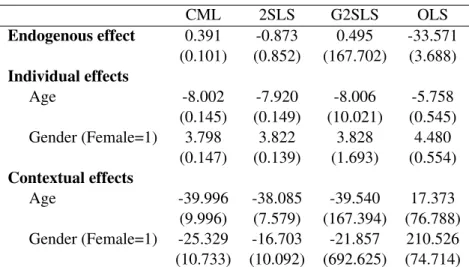
(31) Table 5: Simulations Calibrated on French Sample (1000 replications) Endogenous effect Individual effects Age Gender (Female=1) Contextual effects Age Gender (Female=1). CML 0.391 (0.101). 2SLS -0.873 (0.852). G2SLS 0.495 (167.702). OLS -33.571 (3.688). -8.002 (0.145) 3.798 (0.147). -7.920 (0.149) 3.822 (0.139). -8.006 (10.021) 3.828 (1.693). -5.758 (0.545) 4.480 (0.554). -39.996 (9.996) -25.329 (10.733). -38.085 (7.579) -16.703 (10.092). -39.540 (167.394) -21.857 (692.625). 17.373 (76.788) 210.526 (74.714). Notes: Average standard errors are in parentheses. The group sizes are calibrated on our French sample. 2 = ˆ 2 (calibrated)= 154.704. True value of parameters: Endogenous effect: 0.35; Individual effects - Age: -8; Individual effects - Gender: 3.8; Contextual effects - Age: -40; Contextual effects - Gender: -25.. 28.

(32)