Montréal
Série Scientifique
Scientific Series
2002s-08The Rate of Risk Aversion May
Be Lower Than You Think
CIRANO
Le CIRANO est un organisme sans but lucratif constitué en vertu de la Loi des compagnies du Québec. Le financement de son infrastructure et de ses activités de recherche provient des cotisations de ses organisations-membres, d’une subvention d’infrastructure du ministère de la Recherche, de la Science et de la Technologie, de même que des subventions et mandats obtenus par ses équipes de recherche.
CIRANO is a private non-profit organization incorporated under the Québec Companies Act. Its infrastructure and research activities are funded through fees paid by member organizations, an infrastructure grant from the Ministère de la Recherche, de la Science et de la Technologie, and grants and research mandates obtained by its research teams.
Les organisations-partenaires / The Partner Organizations
•École des Hautes Études Commerciales •École Polytechnique de Montréal •Université Concordia
•Université de Montréal
•Université du Québec à Montréal •Université Laval
•Université McGill
•Ministère des Finances du Québec •MRST
•Alcan inc. •AXA Canada •Banque du Canada
•Banque Laurentienne du Canada •Banque Nationale du Canada •Banque Royale du Canada •Bell Canada
•Bombardier •Bourse de Montréal
•Développement des ressources humaines Canada (DRHC) •Fédération des caisses Desjardins du Québec
•Hydro-Québec •Industrie Canada
•Pratt & Whitney Canada Inc. •Raymond Chabot Grant Thornton •Ville de Montréal
© 2002 Kris Jacobs. Tous droits réservés. All rights reserved. Reproduction partielle permise avec citation du
document source, incluant la notice ©.
Short sections may be quoted without explicit permission, if full credit, including © notice, is given to the source.
ISSN 1198-8177
Les cahiers de la série scientifique (CS) visent à rendre accessibles des résultats de recherche effectuée au CIRANO afin de susciter échanges et commentaires. Ces cahiers sont écrits dans le style des publications scientifiques. Les idées et les opinions émises sont sous l’unique responsabilité des auteurs et ne représentent pas nécessairement les positions du CIRANO ou de ses partenaires.
This paper presents research carried out at CIRANO and aims at encouraging discussion and comment. The observations and viewpoints expressed are the sole responsibility of the authors. They do not necessarily represent positions of CIRANO or its partners.
The Rate of Risk Aversion
May Be Lower Than You Think
*
Kris Jacobs
†Résumé / Abstract
A l’aide de données sur la consommation des ménages et d’équations d’Euler, cet article estime le taux d’aversion au risque relatif. Ces équations d’Euler sont les implications de structures de marché qui ne permettent pas toujours aux agents de s’assurer parfaitement. Cet article porte plus particulièrement sur des tests de l’équation d’Euler inconditionnelle. Dans le cadre d’un agent représentatif, ce type de test mène aux rejets les plus intuitivement convaincants des modèles d’évaluation d’actifs, comme l’énigme de la prime de risque et l’énigme du taux sans risque. Lorsque l’on ignore les erreurs de mesure de la consommation, les erreurs de l’équation d’Euler ne sont pas statistiquement différents de zéro pour les valeurs du taux d’aversion au risque relatif comprises entre 1 et 3. Lorsque l’on tient compte de la présence des erreurs de mesure, les estimations conservatrices du taux d’aversion au risque relatif pour les participants à un marché d’actifs indiquent une valeur entre 2 et 8. Ces résultats suggèrent que le taux d’aversion au risque pourrait être plus bas que ce qui est couramment perçu. Par conséquent, l’imperfection des marchés pourrait servir à résoudre les énigmes d’évaluation d’actifs.
This paper estimates the rate of relative risk aversion using Euler equations based on household-level consumption data. These Euler equations are implications of market structures that do not necessarily allow agents to perfectly insure themselves. The paper focuses on tests of the unconditional Euler equation. In representative-agent frameworks, this type of test leads to the most intuitively convincing rejections of asset-pricing models, such as the equity premium puzzle and the riskfree rate puzzle. When measurement error in consumption is ignored, Euler equation errors are not statistically different from zero for values of the rate of relative risk aversion between 1 and 3. When allowing for the presence of measurement error, conservative estimates of the rate of risk aversion for asset market participants indicate a value between 2 and 8. These findings suggest that the rate of risk aversion may be much lower than commonly thought. Consequently, market incompleteness is likely to be part of a resolution of asset pricing puzzles.
Mots clés : Aversion au risque, Énigme de la prime de risque, Erreurs de mesure, Cohortes synthétiques,
Équations d’Euler, Participation au marché des actifs
Keywords: Risk Aversion; Equity Premium Puzzle; Measurement Error; Synthetic Cohorts; Euler
Equations; Asset Market Participation
JEL : G12
*
Faculty of Management, McGill University and CIRANO. I would like to thank FCAR of Québec and SSHRC of Canada for financial support.
1
Introduction
Asset pricing puzzles such as the equity premium puzzle and the riskfree rate puzzle illus-trate the failure of the representative-agent consumption-based asset pricing models of Lucas (1978) and Breeden (1979) to explain the data. The reason for the widespread interest in these puzzles is probably that they summarize the failure of the model in a way that is intuitively appealing, by referring to mean returns or the ¯rst two moments of returns (e.g. see Mehra and Prescott (1985) and Hansen and Jagannathan (1991)). This failure of the model is easier to grasp intuitively than a statistical rejection.
The focus of this paper is on the importance of incomplete markets structures, and therefore on the measurement of the pricing kernel, for the interpretation of these asset pricing puzzles. In the literature on incomplete markets, the focus has traditionally been on asset-pricing puzzles and less on statistical tests of the model. Early papers (for instance Telmer (1993) and Lucas (1994)) conclude, using a simulation framework, that the impact of incomplete markets on the equity premium puzzle is minimal, because through self-insurance agents end up with consumption allocations that are very similar to those in the complete markets case. Later work by Heaton and Lucas (1996), Constantinides and Du±e (1996), Telmer, Storesletten and Yaron (1997) and Constantinides, Donaldson and Mehra (1998) points out that the impact of incomplete markets depends on a number of issues, such as the persistence of idiosyncratic shocks, the relation of idiosyncratic shocks to aggregate shocks, the net supply of bonds and the speci¯cation of market frictions. The consensus from this literature, which is mostly based on simulation, seems to be that we do not yet have a model that can explain the stylized facts on asset returns, but market incompleteness brings model predictions more in line with the data and therefore holds promise to explain asset pricing puzzles, possibly by incorporating additional rigidities or alternative utility functions.
In a closely related literature, papers by Jacobs (1999), Brav, Constantinides and Geczy (1999), Cogley (1999) and Vissing-Jorgensen (1999) provide additional insight into incom-plete markets structures by testing the incomincom-plete markets framework using data on house-hold consumption. While these tests are of great interest for asset pricing, their interpreta-tion is sometimes problematic because of data limitainterpreta-tions and because simple implicainterpreta-tions of dynamic asset markets such as Euler equations can in principle be tested in many dif-ferent ways. This paper contributes to this literature by investigating the importance of these two potential problems (data limitations and the type of testing technique), which are to some extent interrelated. First, consider the type of test. Jacobs (1999) uses a standard econometric technique to conclude that certain implications of incomplete market models are statistically rejected by the data. Whereas these statistical tests are instructive, they su®er from the same problem as the Hansen and Singleton (1982) tests in the representative agent
literature, because they are intuitively less appealing than the formulation of the model's performance in terms of asset pricing puzzles. This paper attempts to provide additional insight by using household consumption data to construct tests that can be more readily related to the equity premium puzzle and the risk free rate puzzle.
Second, one of the critical problems with the interpretation of tests of Euler equations that use household data is the impact of measurement error in consumption. One of the ways in which such measurement error can be addressed is by loglinearizing the Euler equation, as in Runkle (1991) and Vissing-Jorgensen (1999). This paper investigates a di®erent, more direct approach to the measurement errror problem. Instead of using individual household data to construct the tests, I use data for a consumer that is \representative" for a certain group, such as an age group. For several plausible types of measurement error, this approach will reduce the consequences of the presence of measurement error.
I ¯nd that it is important to take measurement error into account. However, even after allowing for it, the data still indicate moderate degrees of risk aversion. This ¯nding contrasts with ¯ndings in the representative agent literature. Studies of representative agent models that exploit the unconditional Euler equation such as Mehra and Prescott (1985) and Hansen and Jagannathan (1991) typically ¯nd very large values of the rate of relative risk aversion. The paper therefore concludes that the incomplete markets framework holds great promise to explain the equity premium puzzle and the riskfree rate puzzle. The paper proceeds as follows. Section 2 brie°y discusses the evidence on asset pricing puzzles in representative agent models. Section 3 discusses the existing evidence on incomplete markets, outlines the testing methodology and discusses the strategy to deal with measurement error. Section 4 presents the empirical results. Section 5 concludes by discussing the results and outlining future research.
2
Asset Pricing Puzzles in Representative Agent
Mod-els
This paper investigates a set of joint restrictions on security returns and consumption. Con-sider an agent with a time-separable constant relative risk aversion (TS-CRRA) utility func-tion. If the agent maximizes lifetime utility, if she has a riskless and a risky asset at her disposal, and if she does not end up at a corner solution, the following intertemporal Euler equations will hold
1 = ¯Et à ci;t+1 ci;t !°¡1 Rrl;t+1 (1) 1 = ¯Et à ci;t+1 ci;t !°¡1 Rri;t+1 (2)
where ci;t is the consumption of agent i in period t, Rrl;t+1 and Rri;t+1 are the riskless and the risky return between periods t and t + 1; ¯ is the discount factor, Etis the mathematical expectation conditional on information available at t, and 1¡ ° is the rate of relative risk aversion. The theory underlying (1) and (2), coupled with a complete markets assumption, is the basis for much of modern asset pricing theory, and consequently there is substantial interest in testing whether these intertemporal restrictions are supported by the data. If a complete set of markets is available, then individual marginal utility is perfectly correlated with the marginal utility of the representative agent, who consumes aggregate consumption, and one can test the underlying theory by testing (1) and (2), with aggregate consumption taking the place of individual household consumption.
The resulting literature on tests of the representative-agent consumption-based asset-pricing model has shown that the model is at odds with the data in a number of dimen-sions. The early literature (Hansen and Singleton (1982,1983), Grossman, Melino and Shiller (1987)) mainly focuses on the statistical investigation of a number of restrictions implied by the model, and concludes that the model is statistically rejected by the data. Starting with Mehra and Prescott (1985), attention has shifted to well-de¯ned puzzles, aspects of the model which are easily understood intuitively and are clearly at odds with the data. Even though a considerable research e®ort has unearthed a large number of these puzzles, the ones that are most often cited are the equity premium puzzle and the riskfree rate puzzle. The equity premium puzzle, originally pointed out by Mehra and Prescott (1985), states that to explain the di®erence in the return of the risky and the riskless asset, we need risk aversion of the representative agent to be higher than 10, a number which Mehra and Prescott believe to be implausibly high. The riskfree rate puzzle, ¯rst pointed out by Weil (1989), observes that if risk aversion is that high, the discount factor ¯ required to match the historically observed riskfree rate is larger than one.
It must be noted that the equity premium puzzle and the riskfree rate puzzle are not entirely without controversy. To understand this, note that as Kocherlakota (1996) points out, these puzzles are quantitative but not qualitative puzzles. The comovements between the variables of interest in the data conform to the theory, but to match the magnitudes observed in the data, the unobservable parameters of interest ¯ and 1¡ ° have to assume values that are considered implausible. A potential reaction to the puzzles is therefore that judging behavioral parameters as implausible, presumably based on introspection, is not very convincing. In this context, note that Kandel and Stambaugh (1991) argue that fairly high levels of risk aversion may not be implausible, while Kocherlakota (1990) has demonstrated that values of ¯ larger than one can be supported in equilibrium. Whereas this argument is interesting, this paper takes it as given that a large number of economists regard the values of the behavioral parameters as implausible.
These intuitively appealing summaries of the failure of the model have given rise to a very extensive literature. A large part of this literature has focused on changes to the TS-CRRA utility speci¯cation that is used in Mehra and Prescott (1985). As pointed out in a number
of studies (e.g. see Hansen and Jagannathan (1991)), the ¯nding that risk aversion has to be high can be attributed to the fact that the marginal utility of the representative agent is not volatile enough. Consequently, a solution to the puzzle is to make marginal utility more volatile by changing the utility function. Kocherlakota (1996) argues that proposed utility speci¯cations such as habit formation (see Abel (1990), Campbell and Cochrane (1999), Constantinides (1990), Detemple and Zapatero (1991), Ferson and Constantinides (1991), Heaton (1995) and Sundaresan (1989)) and nonexpected utility (see Epstein and Zin (1989,1991) and Weil (1990)) are able to explain the risk free rate puzzle but not the equity premium puzzle. This paper does not discuss empirical evidence on these alternative preference structures, not because they do not have merit, but because the issue of interest is best illustrated using the popular TS-CRRA speci¯cation.
3
Household Consumption Data and Asset Pricing
Puz-zles
3.1
Empirical Methodology
It has long been recognized that incomplete markets structures are a potential explanation of the equity premium puzzle (e.g. see Mankiw (1986) and Mehra and Prescott (1985)). However, the analysis of incomplete markets structures has been conducted using di®erent empirical methodologies. First, a number of studies use simulation techniques. Whereas early quantitative evidence (Aiyagari and Gertler (1991), Huggett (1993), Telmer (1993) and Lucas (1994)) indicates that incomplete markets cannot resolve asset pricing puzzles, it is now recognized that the occurrence of uninsurable risk in a model economy brings predicted asset returns more in line with the data. For instance, Telmer, Storesletten, and Yaron (1997) and Constantinides, Donaldson and Mehra (1999) achieve some degree of success in matching the data using an overlapping-generations framework.
However, the predictions of model economies with incomplete markets depend critically on a number of issues that have to be measured prior to setting up the model to explain asset returns. For instance, the precise measurement of transaction costs is an important issue (see Aiyagari and Gertler (1991), Constantinides (1986), He and Modest (1995), Heaton and Lucas (1995,1996) and Luttmer (1996)). Another important issue is the persistence of idiosyncratic shocks to income (e.g. see Constantinides and Du±e (1996) and Heaton and Lucas (1995, 1996)).1 It must be noted that any future resolution of issues such as 1See also the discussion in Kocherlakota (1996). The issue of persistence is important because it deter-mines the extent to which an individual can insure against income shocks. Given su±cient potential for self-insurance, the outcome of an incomplete markets economy will be similar to that of a complete markets economy (Telmer (1993)). It must be noted that a model economy with high shock persistence has implica-tions similar to a model economy where the number of shocks is small in comparison to the individual's life
the persistence of income shocks requires a careful analysis of household-level data, and therefore simulation-based studies are subject to similar criticism about data limitations as direct statistical analyses of household-level data.
A second approach to analyzing market incompleteness focuses on restrictions implied by the model under a weaker set of assumptions, such as restrictions (1) and (2). This is the approach followed in this paper. Besides providing a valuable complement to simulation-based studies, parameter estimates obtained through this analysis are also of interest as inputs in simulations or calibrations. To motivate the empirical analysis in this paper and to see the link with existing studies, consider the following framework. Consider the errors u1
i;t and u2i;t associated with the Euler equations (1) and (2), where t is the time index and i is the household index. Theory speci¯es Et¡1u1
i;t = Et¡1u2i;t = 0: The equity premium puzzle and the riskfree rate puzzle can then be understood using the expressions E u1
i;t= E u2
i;t = 0; which are readily obtained using the law of iterated expectations: First consider the corresponding restrictions in the representative-agent case. In this case E u1
t = E u2t = 0: There is no i subscript: the theory speci¯es only two orthogonality conditions. Therefore, in the representative-agent case, we have a just identi¯ed econometric problem: two equations in the two unknowns ¯ and 1¡ °.
The incomplete markets case we analyze in this paper can be cast in a similar setup. In this case we have a maximum of T observations on N households. In contrast to the rep-resentative agent problem, the optimization problem using household data is overidenti¯ed: we have 2£ N restrictions to determine 2 parameters. However, these 2 £ N orthogonality restrictions can conveniently be reduced to 2 orthogonality conditions in an intuitively ap-pealing way. Noting that the panel is unbalanced, denote the number of households in the sample at time t as Nt. We can simply use the two orthogonality conditions E u1t and E u2t where ujt = (1=Nt)PNi=1t u
j
i;t, which gives us two equations in two unknowns.
It is possible to provide more intuition by further relating this setup to the existing literature using a generalized method of moments (GMM) framework. See Campbell, Lo and MacKinlay (1997), Cochrane (2001) and Ferson (1995) for a more in-depth treatment. In the representative agent case one can think of the errors u1
t and u2t associated with the Euler equations as pricing errors. In the incomplete markets case u1
t and u2t are average pricing errors. The type of analysis that is directly based on the pricing errors is often referred to as the analysis of the unconditional Euler equation. Now consider the same sample with a maximum of T observations on N households and consider an instrument zi;t¡1 (notice that for simplicity the instrument does not carry a superscript, to indicate that we can use the same instrument for both equations). Then consider "1
i;t = u1i;tzi;t¡1 and "2
i;t = u2i;tzi;t¡1: Using the law of iterated expectations we know that E "1i;t = E "2i;t = 0, for all i. We therefore again have 2£ N orthogonality conditions, which can be reduced to
span. This partly explains the success of the overlapping generations models in Telmer, Storesletten, and Yaron (1997) and Constantinides, Donaldson and Mehra (1999).
two orthogonality conditions E "1
t and E "2t where "jt = (1=Nt)PNi=1t " j
i;t: If the instrument zi;t¡1 depends on time (such as asset returns or consumption growth), the resulting analysis is referred to as exploiting the conditional Euler equation. Another way this is referred to in the literature is as an analysis of \scaled" pricing errors or as a payo® to a \managed portfolio" (Cochrane (2001)). In contrast, the analysis of the unconditional Euler equation described above analyzes the \unscaled" pricing errors. Another way to interpret this is as an analysis of scaled pricing errors where the \scaling" instrument zi;t¡1 is a constant.
The GMM framework looks at two theoretical restrictions such as E u1
t = E u2t = 0 or E "1
t = E "2t = 0 as two orthogonality conditions, regardless of whether they originate from representative agent problems or incomplete markets problems and regardless of whether the instrument zi;t¡1 is time-varying. The GMM approach exploits the fact that if the theory can explain the data, the sample equivalent of these orthogonality conditions should be zero. At its most general, consider the restrictions implied by an incomplete markets economy with a time-varying instrument zi;t¡1. De¯ne the 2£ 1 vector "t= ("1t; "2t)0 and consider the minimization problem JT = [ 1 T T X t=1 "t(Á)0] W [ 1 T T X t=1 "t(Á)]: (3)
where Á denotes the (2£ 1) parameter vector and W is a weighting matrix. The equity premium puzzle can be cast in this statistical framework by observing that the corresponding minimization problem (3), when using aggregate data and when using a constant as an instrument, yields large levels of risk aversion and a value of ¯ larger than one. The question addressed by this paper asks if the corresponding minimization problem using household data yields more plausible parameter values. It must be noted that to obtain consistent estimates of the parameters ¯ and 1¡ °, one can actually analyze "t = ("1t; "2t)0 instead of minimizing (3), because the problem is just identi¯ed. Therefore, to ¯nd the parameter values, we can solve "t = ("1t; "2t)0 using a nonlinear solution algorithm, and we do not necessarily have to analyze (3). A valid solution to the optimization problem (3) is one for which "t = ("1t; "2t)0 is exactly zero.2 However, for analyses of the conditional Euler equation that use more instruments zi;t¡1, this is not the case. For instance, if we consider the Euler equations (1) and (2) and use two lagged instruments for each Euler equation, we end up with four orthogonality conditions to determine the two parameters. The problem is then overidenti¯ed and can only be analyzed by minimizing (3). In this case the choice of the weighting matrix W is critical, while it is of no consequence for a just-identi¯ed problem. See Hansen and Singleton (1982) and Jacobs (1999) for econometric analyses of overidenti¯ed problems in the representative agent and incomplete markets cases respectively.
2This statement of course has to be understood to mean that the Euler equation errors are arbitrarily close to zero. The same is true for the objective function in (3).
3.2
Interpreting Asset Pricing Puzzles
A few more observations about the interpretation of the equity premium puzzle and the risk-free rate puzzle are in order which are most conveniently illustrated using a GMM framework. First, in the case of the equity premium puzzle, since we are dealing with a just identi¯ed GMM problem it is clear that we cannot test the theory in a formal econometric sense. We have just enough orthogonality conditions available to estimate parameters and compute standard errors. It is therefore clear that in the context of this GMM optimization problem the equity premium puzzle has to be seen as a statement about the plausibility of estimated parameters. Second, when considering the risk free rate puzzle from the perspective of some well-de¯ned GMM problem, since we have one equation with two parameters, the problem is underidenti¯ed. So not only can we not test the theory econometrically, in principle we cannot obtain estimates of the behavioral parameters either. The caveat, clearly expressed in the literature, is of course that when discussed in this context, the risk free rate puzzle is a puzzle conditional on the existence of the equity premium puzzle (e.g. see Campbell, Lo and MacKinlay (1997), Kocherlakota (1996)). Conditional on large risk aversion, the Euler equation associated with the riskless asset implies an implausible discount rate. So in the context of the GMM problem above, once we have an estimate of 1¡°, we have one equation in one remaining unknown, a just identi¯ed problem.
However, the asset-pricing literature also contains a number of techniques and analyses which provide a slightly di®erent formulation of asset-pricing puzzles. In the GMM setup described above, the Euler equations for the riskless and the risky asset yield two Euler equa-tions in the representative agent context. The reason why we are not able to test the model statistically is that we choose to use these two orthogonality conditions to obtain inference on the two parameters. Alternatively, conditional on knowledge of the parameter values, we have two overidentifying conditions available to test the model. Even the risk-free rate puzzle becomes testable econometrically, since it becomes a problem with one overidentifying condition. Therefore, we can construct tests of these asset pricing models conditional on a wide range of parameter values. Asset pricing puzzles are then slightly restated but intu-itively similar: instead of using the data to infer parameter values, and then judge whether these parameter values are plausible, we construct econometric tests of Euler equation errors conditional on a range of parameter values, and then ask ourselves if those parameter values that imply Euler errors that are statistically indistinguishable from zero are plausible. The simplest possible implementation of this methodology is illustrated in Kocherlakota (1996). Whereas that paper constructs univariate t-tests, in principle multivariate chi-square tests can be constructed. Indeed, to use multivariate information in an optimal way, GMM-type testing conditional on the behavioral parameters can be used (see Burnside (1994), Cecchetti, Lam and Mark (1994) and Hansen, Heaton and Luttmer (1995)). To some extent, this can be interpreted as an application of incorporating prior information, with the prior either resulting from introspection, or from other (related) information. Although they have a
dif-ferent focus than the analysis in Kocherlakota (1996), the techniques advocated by Hansen and Jagannathan (1991) use a similar setup. These graphical techniques focus on values of behavioral parameters needed to match the ¯rst and second moments of asset returns. For instance, using only the riskfree asset we ¯nd that for a \plausible" value of ¯ of 0:95; \implausible" levels of risk aversion are needed to match the riskfree rate. This paper follows a similar approach to analyze the incomplete markets case using panel data. The tests are based on overidenti¯ed GMM problems such as (3), which lead to tests of the models using Â2 statistics.
3.3
Measurement error
The estimation and analysis of (1) and (2) using data on individual household consumption assumes that the available data are measured without error. We know that for panel data this is unlikely to be the case (see Altonji (1986) and Altonji and Siow (1987)). While it is by de¯nition impossible to remove this measurement error from the data, there are a number of alternatives available to reduce its consequences. One potential solution is to loglinearize the Euler equations, as in Runkle (1991) and Vissing-Jorgensen (1999). Such a loglineariza-tion can be justi¯ed by relying on a Taylor series approximaloglineariza-tion or by assuming that the distribution of the data is jointly lognormal, and it can resolve measurement error problems given appropriate instrumentation. While this is an interesting approach, the disadvantage is that if the assumptions underlying the loglinearization are incorrect, the resulting test statistics and parameter estimates will be biased. Another potential technique to assess the implications of measurement error is to assume a functional form for the measurement error and to use simulation techniques to investigate its impact on the test statistics. This ap-proach is followed by Vissing-Jorgensen (1999) and Brav, Constantinides and Geczy (1999). While this is an interesting approach, its validity is predicated on assuming the correct type of measurement error.
In this paper I propose to use synthetic cohorts to reduce the negative impact of measure-ment error. Synthetic cohorts have been used in the economics literature for a long time.3 The approach requires the construction of cohorts, groups of individuals with comparable characteristics. For instance, one often used approach is to form cohorts based on age. For each age group, we construct a \representative" individual who has data associated with him/her that are the average of the data in that age group. It is clear that this is also an imperfect solution to the measurement error problem. If the consumption growth of one of the individuals in a certain age group is measured with error, the measurement error is not eliminated. Instead, the relative importance of the measurement error is reduced by averaging it out using other observations. Moreover, it must be noted that the formation of
3The traditional motivation for using the synthetic cohorts technique is somewhat di®erent. It has mainly been used because many available panels are too short for the analysis of rational expectations models (see Browning, Deaton and Irish (1985) and Attanasio and Weber (1995)).
synthetic cohorts can also adversely a®ect the analysis. The central thesis of the market incompleteness literature is that the study of representative agent data is to some extent uninformative because variability in individual marginal rates of substitution is averaged out when studying the marginal rate of substitution of the representative consumer. When constructing synthetic cohorts, one runs into the same problem that besides averaging out the e®ects of measurement error, one also averages out genuine volatility in marginal rates of subsitution. In fact, the construction of a representative agent can be seen as the extreme of synthetic cohorts construction, with just one cohort. As a result, one partially reduces the consequences of measurement error, but at the cost of introducing a new problem. The synthetic cohort approach can therefore be interpreted as ¯nding a middle way between the problems associated with using individual data (measurement error) and the problems associated with the representative agent approach (eliminating MRS variability).
In the empirical work, I use synthetic cohorts based on relatively large groups, which presumably eliminate most of the measurement error. Because such a construction also eliminates some genuine MRS variability, the resulting parameter estimates can usefully be interpreted as conservative estimates of the rate of risk aversion. I ¯rst construct synthetic cohorts by sorting on the age of the household head. I use households where the household head is aged between 25 and 60; resulting in 36 cohorts. I provide a robustness check by also constructing synthetic cohorts using the household head's education as well as his age, using 12 age categories and 2 educational categories. This results in 24 cohorts. In principle, it is possible to conduct further robustness checks by using interesting variables such as household wealth and household income as sorting variables. The analysis in this paper is limited to the two sorts described above to keep the presentation of the evidence manageable.
There is one remaining issue regarding the cohort construction. The main variable of interest in this study is consumption growth. For each cohort group, we therefore con-struct an average consumption growth variable. However, this can be done in (at least) two di®erent ways. First one can construct the cohort consumption level and then use the cohort consumption level to compute cohort consumption growth. More precisely, given individual consumption ci;t the consumption of a representative cohort j at time t is given by ccoj;t = (1=Nj;t)PNi=1j;tci;t, where Nj;t is the number of observations in this cohort at time t. Consumption growth for the cohort is then computed as ccog1;j;t = (ccoj;t=ccoj;t¡1) Alternatively, one can compute cohort consumption growth by averaging over individual consumption growth of the cohort members. More precisely, ccog2;j;t = (1=Nj;t)PNi=1j;t(cgi;t) where cgi;t = ci;t=ci;t¡1:
3.4
Related Literature
Besides the literature on incomplete markets referred to in section 3.1, there are a number of studies that are related to the empirical work in this paper. First, the complete markets assumption has been strongly statistically rejected in a number of recent studies (see
Attana-sio and Davis (1997), Cochrane (1991), Mace (1991), Hayashi, Altonji and Kotliko® (1996); see Altug and Miller (1990) and Miller and Sieg (1997) for con°icting evidence). Second, Mankiw and Zeldes (1991) investigate the impact of asset market participation on the equity premium puzzle. They are motivated by aggregation results that hold only for asset market participants (see Grossman and Shiller (1982)). Therefore, they use panel data to eliminate non-assetholders from the sample and investigate if the resulting per capita consumption of assetholders di®ers from per capita consumption for all households. Mankiw and Zeldes (1991) also obtain inference on parameters by analyzing the unconditional Euler equation. However, because of their setup, they obtain inference on the rate of risk aversion but not on the discount rate ¯. Also, the analysis focuses on per capita (average) consumption and not on the properties of individual household consumption; however, the properties of per capita consumption are dramatically di®erent from the properties of household consumption or cohort consumption, suggesting that the assumptions necessary for aggregation of those households at interior conditions are not validated by the data. While the use of per capita consumption based on panel data presumably avoids most of the measurement error prob-lems associated with individual consumption, it seems desirable to investigate the dispersion in marginal rates of substitution in the cross-section.
Third, by focusing on individual household consumption, some of the results in this pa-per are also intimately related to certain ¯ndings in the life-cycle literature, for instance in the papers by Attanasio and Browning (1995), Attanasio and Weber (1993,1995), Hall and Mishkin (1982), Runkle (1991) and Zeldes (1989). These papers typically investigate linearizations of the conditional Euler equation associated with the riskless asset. Altug and Miller (1990) use panel data to investigate nonlinear Euler equations under the maintained hypothesis of market completeness. Finally, Jacobs (1999) investigates Euler equations (1) and (2) without making a market completeness assumption. That study focuses on overi-denti¯ed estimation problems which allow statistical tests of the model. The overidentifying conditions are obtained from the conditional Euler equation. Jacobs (1999) ¯nds that the consumption-based asset pricing model is statistically rejected by the data along several di-mensions. Estimates of behavioral parameters are robust across estimation exercises, with fairly plausible inference on the discount rate as well as the rate of relative risk aversion.
Whereas the results in the life-cycle literature and in Jacobs (1999) are insightful, more evidence on asset pricing puzzles is desirable by focusing exclusively on the unconditional Euler equation. To motivate this, a reference to the empirical evidence in the representative agent literature is instructive. The results in Jacobs (1999) are obtained using panel data and an incomplete markets assumption using similar information as exploited by Hansen and Singleton (1982) in a representative agent framework. Hansen and Singleton (1982,1984) reject the model statistically and obtain estimates of the rate of relative risk aversion that are in most cases intuitively plausible.4 Estimates of the discount rate are very precise and 4However, some of the estimates of the rate of relative risk aversion in Hansen and Singleton (1982, 1984)
in most cases intuitively plausible. However, the work of Hansen and Singleton (1983), Mehra and Prescott (1985), Grossman, Melino and Shiller (1987) shows that if only the unconditional Euler equation is used in the representative agent framework, inference on the rate of relative risk aversion changes dramatically. Indeed, by using the unconditional Euler equation one obtains the equity premium puzzle and the implied risk aversion is very high. This ¯nding is con¯rmed using the tools developed by Hansen and Jagannathan (1991). So obviously the type of information used is critical in representative agent studies, and this could very well be the case when using household level data. The focus of this paper is therefore to verify if the intuitively plausible estimates of the rate of relative risk aversion obtained in Jacobs (1999) are con¯rmed when only unconditional information is used and when measurement error is taken into account. As explained above, this is of substantial interest because implicitly or explicitly, the validity of asset pricing theories has been judged by these parameter values. It must be noted that the studies by Brav, Constantinides and Geczy (1999), Cogley (1999) and Vissing-Jorgensen (1999) give partial answers to some of these questions. These studies seem to indicate that measurement error has potentially serious implications and that risk aversion is lower than in representative agent studies, although the estimates di®er considerably between papers.
4
Empirical Results
4.1
Data
The data used in the analysis are consumption data from the Panel Study of Income Dy-namics (PSID) that are also used in Jacobs (1999). I refer the reader to Jacobs (1999) for a detailed discussion of the data; here I provide a brief summary. The data are taken from the 1987 PSID ¯les and allow construction of consumption growth rates for the period 1974-1985. The empirical analysis is repeated for four di®erent samples. The ¯rst sample consists of all households who ful¯ll a set of sample selection criteria. This dataset contains 3555 households and 18813 total observations (note that the panel is unbalanced: a household can be in the sample one year and not in another year). This sample is referred to as sample 1, but a problem with this sample is that some of the households do not hold assets. Including such households in the sample is likely to bias the results. I therefore use three smaller sam-ples that contain only assetholders. A second sample (referred to as sample 2) includes only households that report nonzero holdings of the riskless and the risky asset. It contains 740 households and 5029 total observations. A third and fourth sample (referred to as samples 3 and 4) contain only households that report holdings of the riskless and risky assets larger than $1,000 and $10,000, respectively. These datasets contain 413 and 103 households and
are in the nonconcave region of the parameter space and the estimates are imprecise for several estimation exercises.
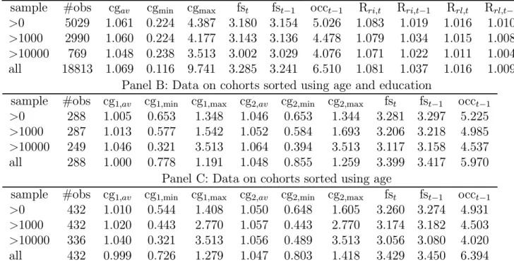
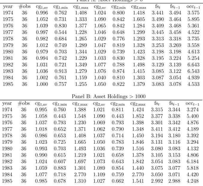
2990 and 769 total observations, respectively. Table I provides descriptive statistics for these samples (in panel A) as well as for the samples synthetic cohorts based on them (in panels B and C).5 Table IA indicates that sample 1 (the one containing all households) contains more extreme outliers compared to the other samples. However, this may be partly due to the fact that it is the largest sample. Another observation is that the cohort construction signi¯cantly alters the properties of the di®erent datasets, as can be seen from a comparison of table IA with tables IB and IC.
4.2
Asset Pricing Puzzles Under Incomplete Markets
We obtain inference on the equity premium in incomplete markets for the four samples described above by analyzing ut = (u1t; u2t)0, which is a system of two equations in two unknowns, for each of these samples. Intuititively this analysis indicates whether we can ¯nd values of the parameters ¯ and 1¡ ° that can explain the average (across households) Euler equation pricing errors for the riskless and the risky asset. However, there is an additional empirical problem with household level consumption data in this context which has not yet been discussed. Whereas the Euler equations (1) and (2) are de¯ned for an individual agent, consumption data are available at the household level. In principle this issue is easily addressed by including a function of household size in the Euler equation. We can estimate 1 = ¯Et à ci;t+1 ci;t !°¡1
Rrl;t+1exp(f1f si;t+1+ f2fsi;t) (4)
1 = ¯Et Ã
ci;t+1 ci;t
!°¡1
Rri;t+1exp(f1f si;t+1+ f2fsi;t) (5) where fsi;t stands for family size in period t and f1 and f2 are scalar parameters. However, this means four parameters to estimate and the Euler equations for the riskless and the risky asset give us only two orthogonality conditions, when using a constant as the sole instrument. The problem is underidenti¯ed. We can solve this problem in two ways. First, we can include current and lagged household size in the instrument set, to yield four equations in four unknowns. The approach I follow instead is to plug in estimates of f1 and f2 that are obtained from the estimation of overidenti¯ed or just identi¯ed estimation problems implied by (4) and (5). This results in a just-identi¯ed problem of two equations in two unknowns. It was veri¯ed that estimates of f1 and f2 are robust across estimation exercises, and do not in°uence the empirical results.
Results on the equity premium puzzle are presented using a graphical tool that is in the same spirit as the tables in Kocherlakota (1996). Instead of conducting an econometric
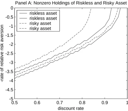
analysis and evaluating the parameters using the results of econometric estimation, we eval-uate the orthogonality restrictions for a number of combinations of the parameter values, and subsequently ask if any of the parameter values for which the theory is not rejected is intuitively plausible. To facilitate the interpretation of the results on incomplete markets obtained with this alternative technique, ¯gure 1 analyzes the Euler equation errors for the more familiar representative agent case, using the Mehra and Prescott (1985) annual data for 1889-1979. Figure 1C summarizes the information in the sample equivalents to the Euler equations in the way it is going to be used in the rest of the paper. This ¯gure summarizes the information contained in ¯gures 1A and 1B. To save space the counterparts to ¯gures 1A and 1B are omitted in the ¯gures that analyze household data.
Figure 1A presents a grid where the inputs are the discount rate and the rate of relative risk aversion. For the discount rate ¯ values between 0.5 and 1.1 are analyzed. For ° ¡ 1 (the negative of the rate of relative risk aversion) we limit our attention to values between -50 (in the concave region of the parameter space) and +20 (in the nonconcave region of the parameter space). The vertical axis represents the negative of the absolute value of the average Euler equation error for the riskless asset. Therefore, this grid reaches a maximum value of zero for parameter combinations that solve the Euler equation for the riskless asset. We can therefore conduct the following informal exercise: pick an a priori reasonable value of ¯ and verify what level of risk aversion is necessary to solve the Euler equation. Many economists would argue that values of beta between 0.8 and 1 are intuitively plausible. Given these values and the data, a solution to the Euler equation is given for relative risk aversion of approximately 25 to 35, which many economists consider implausibly high. Figure 1B presents the same analysis for the Euler equation associated with the risky asset. Again, given plausible discount rates we need very high rates of risk aversion to solve the Euler equation. Note that for a given plausible discount rate, the risk aversion needed to match the riskless rate is slightly lower than the one needed to match the risky rate.
Figure 1C presents the information contained in ¯gures 1A and 1B in a more parsimonious way. This ¯gure has the discount rate on the horizontal axis and risk aversion on the vertical axis. The triangles and squares present combinations of the parameters that make the Euler equations for the risky and the riskless asset respectively equal to zero.6 For all values of ¯ smaller than one, the squares are above the circles. In other words, it is not possible to ¯nd a parameter combination that solves both Euler equations as long as the discount rate
6Because ¯gures 1A and 1B are in fact created using a grid, the \ridge" in these ¯gures that suggests zero Euler equation errors is in fact a locus of very small Euler equation errors. It was veri¯ed that actual solutions to the equations exist in the neighbourhood of the parameter values in the grid. Presenting a ¯ner grid does not provide any additional insight. With respect to ¯gure 1C, note that the \solutions" pulled of the grid are therefore \near" solutions. This ¯gure could be made more precise by presenting a locus of exact solutions, but again this does not provide any additional insight. After all, whether a relative risk aversion of 30.32 or 30.36 is needed to match the restrictions of the model is not likely to in°uence our assessment of the model's performance.
is smaller than one. When ¯ is allowed to be larger than one, a solution to the system of equations can be found, namely for a discount rate approximately equal to 1.08 and a rate of relative risk aversion approximately equal to 23. As extensively discussed above, these values are judged to be implausible. What is perhaps not clearly indicated in the representative agent literature is the fact that, for values of the discount rate only slightly higher than 1.08, it is impossible to ¯nd a rate of risk aversion that solves the Euler equations for the risky and riskless asset separately (let alone jointly).7
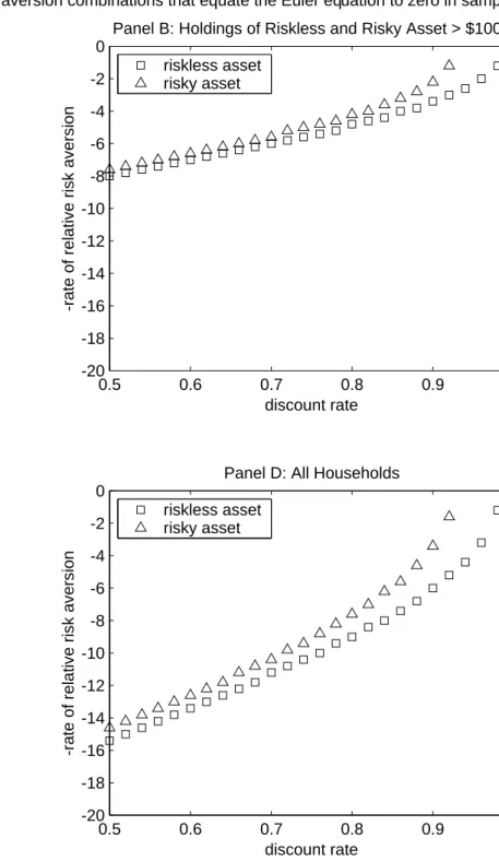
We now turn to similar graphical analyses of the restrictions imposed by the incomplete markets models on the data for individual households. Figure 2 presents information for the four individual household samples similar to that in ¯gure 1C. Figure 2A reports on the sample of households that report nonzero holdings of the riskless and risky assets, and ¯gures 2B and 2C report on those households with holdings of the riskless and risky asset in excess of $1,000 and $10,000 respectively. Finally, ¯gure 2D presents results for the complete sample of 18813 observations.8
Figure 2 clearly indicates that parameter combinations needed to solve each Euler equa-tion separately are much more plausible than in the representative agent model. Most importantly, compared to the representative agent model, the data point towards lower risk aversion. For most plausible values of the discount rate, the rate of relative risk aversion implied by the data is between 0.5 and 3. With respect to discount rates, whereas in the representative agent case solutions to separate Euler equations do not exist for discount rates larger than 1.1, for the household level data we cannot obtain solutions to the Euler equation for the risky asset for ¯ larger than 0.9, and to the Euler equations for the riskless asset for
7In a sense, the representation of asset pricing puzzles in ¯gure 1C is superior to simply reporting the results of an econometric estimation exercise. The ¯gure has an advantage similar to an often used repre-sentation of the Hansen-Jagannathan (1991) bounds, because in essence the test information is repeated for many di®erent parameter combinations, and not exclusively for the parameter combination that minimizes a given objective function. In some sense, the information in ¯gure 1C is also superior to Hansen-Jagannathan (1991) bounds, because those bounds only use the ¯rst two moments of the IMRS. However, all these per-ceived advantages over other testing methods have to be put in perspective. The representation of asset pricing puzzles in ¯gure 1C is convenient because in the case of a CRRA speci¯cation we are dealing with a two-parameter problem. Tools such as the Hansen-Jagannathan bounds and GMM estimation are designed to deal with richer parameterizations of the utility function (see Heaton (1995) and Cochrane and Hansen (1992)). Therefore, whereas the graphical tool used in ¯gure 1C may be useful in the context of this paper, it is of limited use more generally.
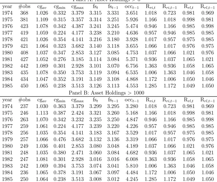
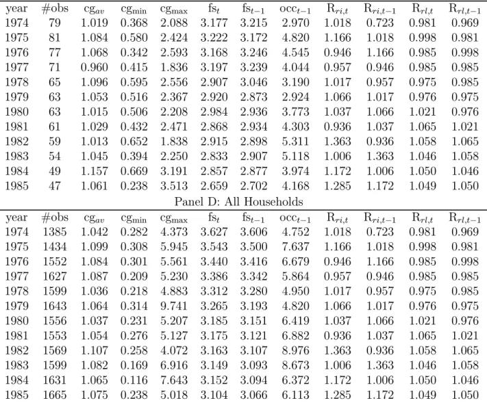
8To provide some additional insight into the properties of the four samples, table II provides descriptive statistics on a year-by year basis. This complements the descriptive statistics in table IA, which are for the entire sample. Table II indicates that there is quite a bit of variation in the risky rate of return over the sample period. When comparing the four di®erent samples, average consumption growth rates on a year-by-year basis are fairly similar. The minima and maxima for consumption growth are more extreme for the sample that contains all households, but it has to be kept in mind that this sample is larger, and therefore more likely to contain extremely high and low growth rates of consumption. In terms of measurement error, it must be noted that there seem to be very few extreme outliers, even though no consumption growth criterion was used to screen observations.
¯ larger than 0.95.
It is somewhat surprising that for the sample that includes non-assetholders (¯gure 2D) implied risk aversion is not much di®erent from ¯gures 2A, 2B and 2C. Studies by Constan-tinides, Brav and Geczy (1999), Vissing-Jorgensen (1999), and Mankiw and Zeldes (1991) suggest that the distinction between assetholders and non-assetholders is important. The evidence presented in ¯gure 2 suggests that the issue of aggregation is much more important than the inclusion of non-assetholders in the sample. If the presence of non-assetholders in the sample is an important issue, we would expect to see an implied rate of risk aversion in ¯gure 2D that is more similar to the ones implied by representative agent models, and therefore much higher than the ones in ¯gures 2A, 2B and 2C.
There is another important stylized fact in ¯gure 2 which requires elaboration. While there is a large number of intuitively plausible combinations of ¯ and 1¡ ° for which each of the Euler equations can be solved, there is no combination of ¯ and 1¡ ° that solves both Euler equations simultaneously. In the ¯gures, such a parameter combination would be represented by an intersection of the lines formed by the triangles and the squares. For instance, in the representative agent case in ¯gure 1C there is such a case, but only for an implausible parameter combination with ¯ larger than 1 and a large value for the rate of relative risk aversion.9
What does this ¯nding mean? Asset pricing puzzles in the representative agent model are often summarized by the ¯nding in ¯gure 1C that is summarized above: a \calibration" of the model using both Euler equations yields an exact solution to the system of equations for a discount rate approximately equal to 1.08 and a rate of relative risk aversion approximately equal to 23. Of course, the puzzle is much deeper. Figure 1 clearly indicates that for almost all reasonable discount rates, the rate of risk aversion implied by either Euler equation is very large. The relevant question is not whether the particular values \calibrated" on the system of two equations in two unknowns are plausible, but whether there are any parameter combinations for which both Euler equation errors are statistically indistinguishable from zero. This is the approach followed in most of the literature (see for instance Kocherlakota (1996) and also (in a di®erent context) Hansen and Jagannathan (1991) and Cochrane and Hansen (1992)). We therefore turn to a similar analysis for incomplete markets involving the PSID household-level data.
9As mentioned above, ¯gure 2 represents systems of two equations in two unknowns. In principle therefore, to ¯nd the parameter values implied by the data, we can solve "t = ("1
t; "2t)0 using a nonlinear solution algorithm. Alternatively, we can analyze (3) which should have a minimum of zero if there is an exact solution. Figure 2 indicates that whereas (3) has a minimum, at this minimum "t = ("1
t; "2t)0 is not zero. This ¯nding is corroborated by an extensive grid search and a search using a nonlinear solution algorithm, which indicates that there are no exact solutions.
4.3
Statistically signi¯cant Euler equation errors
Figure 3 extends the graphical representation of the Euler equation errors in ¯gure 2 to illus-trate all parameter combinations for which the Euler equations are not statistically di®erent from zero. Figure 3A presents results for sample 2, ¯gure 3B for sample 3, ¯gure 3C for sample 4, and ¯gure 3D for sample 1. Each ¯gure contains two solid lines and two broken lines. The area between the two solid lines is the area for which the Euler equation for the riskless asset is statistically indistinguishable from zero.10 The area between the broken lines indicates the area for which the Euler equation for the risky asset is statistically indistin-guishable from zero. Therefore, any overlap between these two areas can be interpreted as a set of parameter combinations for which the equity premium is resolved.11
Each of the ¯gures contains such an overlap between the statistically signi¯cant solution for the riskless asset and the risky asset. In all samples, the number of parameter combina-tions that solves the Euler equation is much larger for the risky asset. As expected, the areas that solve the Euler equations are largest in ¯gure 3C, the ¯gure for the smallest sample, because this sample contains the smallest amount of information.12 Once again it is the case that ¯gure 3D, which also includes non-assetholders, looks very similar to ¯gures 3A, 3B and 3C.
For the sake of comparison, ¯gure 1D provides a similar analysis for the representative agent framework, using the Mehra-Prescott (1985) data. Note that this ¯gure contains only 1 solid line and 1 broken line. For a given discount rate, if the null hypothesis of a zero Euler equation error cannot be rejected for a certain rate of relative risk aversion, it can also not be rejected for any larger rate of relative risk aversion (this was veri¯ed only for rates of risk aversion smaller than 70). Therefore, ¯gure 1D indicates that even though there is only one parameter combination that solves the system of two equations in two unknowns (see ¯gure 1C), there are many parameter combinations for which the hypothesis that either Euler equation is zero cannot be rejected (tested separately). However, these parameter combinations always involve a rate of relative risk aversion which is considered implausibly high. The equity premium puzzle is very robust in representative agent models because, even
10As explained above, the statistical tests are based on the GMM framework. The orthogonality condition E u1
t can be interpreted as 1 equation in two unknowns, ¯ and 1¡ °, and is therefore underidenti¯ed. However, conditional on given values of ¯ and 1¡ °; we have 1 overidentifying condition, which can be used to construct a Â2
1 statistic. To construct this statistic, it is assumed that the Euler equation errors for a household are uncorrelated over time. The correlation between di®erent households at the same point in time is determined by the size of the aggregate shock hitting the economy at that time, and therefore it is allowed to be nonzero.
11Strictly speaking, one should construct a joint test for the hypothesis that both Euler equation errors are nonzero. I present univariate tests because they facilitate the graphical presentation of the results.
12This of course also illustrates the conventional problem that test statistics that are statistically not distinguishable from zero may result from a lack of su±cient data and therefore from a lack of power of the test.
though we can ¯nd a wide range of parameter values for which the Euler equation errors are statistically indistinguishable from zero (not just the one parameter combination indicated by GMM), all these parameter combinations are judged implausible.
4.4
Analysis of Cohort Data
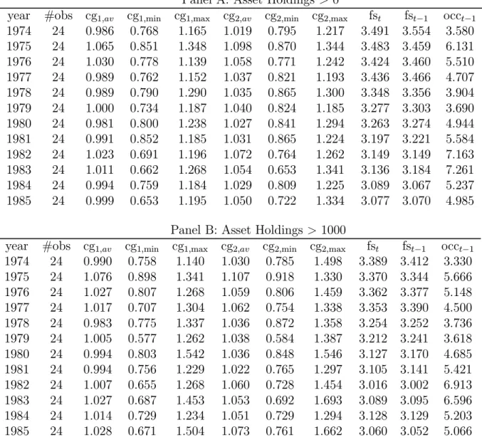
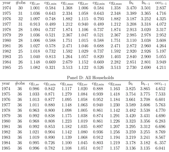
Figures 4 through 7 present an analysis of the Euler equation errors for cohort data. Figures 4 and 5 present results for cohorts formed on the basis of age and education. Figures 6 and 7 present results for cohorts formed on the basis of age. Figures 4 and 6 use cohort consumption growth that is obtained by ¯rst obtaning the consumption levels of a representative cohort, and subsequently computing the cohort's consumption growth. Figures 5 and 7 obtain cohort consumption growth by averaging over individual consumption growth. Each ¯gure contains four panels, corresponding to samples 2, 3, 4 and 1. To further motivate the analysis of the cohort data, it is instructive to compare the descriptive statistics for the cohort data in tables III and IV with the descriptive statistics for the individual data in table II. It is clear that there are important di®erences in the properties of the consumption growth data. Regardless of the method used to construct cohort consumption growth, the cohort consumption growth data contain far fewer outliers than the individual data in table II. A few other stylized facts should be mentioned. First, average growth rates are always higher when computed by averaging over individual growth rates as opposed to averaging over the consumption levels. Second, because the cohort statistics in table IV are obtained using more cohorts, the distribution of consumption growth is more spread out than in table III. These stylized facts are also clear from comparing tables IB and IC.
Inspection of ¯gures 4 through 7 yields three important general conclusions. First, implied rates of risk aversion are higher than for the individual data in ¯gure 2, but dra-matically lower than for the representative agent data in ¯gure 1. Second, the implied rate of risk aversion is lower for assetholders than for non-assetholders. In panel D, the rate of risk aversion is implausibly large for plausible values of the rate of time preference. I therefore conclude that the inclusion of non-assetholders likely biases estimates of the be-havioral parameters. This ¯nding is in accordance with existing ¯ndings in Mankiw and Zeldes (1991), Constantinides, Brav and Geczy (1991) and Vissing-Jorgensen (1999). This conclusion di®ers from the ¯ndings in ¯gure 2, which were obtained using individual data. In ¯gure 2, di®erent samples indicate comparable rates of risk aversion, regardless of whether non-assetholders were included in the sample or not. It is therefore reasonable to conclude that there is substantial measurement error in individual consumption data, and that this measurement error is (partially) eliminated by the representative cohort construction.13
13There is one important caveat in interpreting these ¯gures, which is the di®erences in the sizes of the cohorts used to generate the ¯gures. Because the samples get smaller as we consider households that hold larger asset portfolios (see tables I and II), the average cohorts used to generate panel C in ¯gures 4 through 7 are always smaller than those used to generate panel A in ¯gures 4 through 7. To investigate the impact
Third, di®erent samples of assetholders imply di®erent rates of risk aversion. In each of the four ¯gures, we see that panel A has the highest rates of risk aversion, with risk aversion getting smaller as we consider households that hold larger amounts of assets.14 Again, this ¯nding is in accordance with existing research (see Mankiw and Zeldes (1991), Constantinides, Brav and Geczy (1991) and Vissing-Jorgensen (1999)). What estimate of risk aversion should we then remember from these ¯gures? Not all rates of time preference investigated in these pictures are intuitively plausible: many economists would argue that ¯ should be at least 0.85 or even 0.9. For those calues of ¯, the ¯gures indicate a rate of risk aversion of no higher than 8 and in several cases as low as 2.
4.5
Analysis of Representative Agent Data
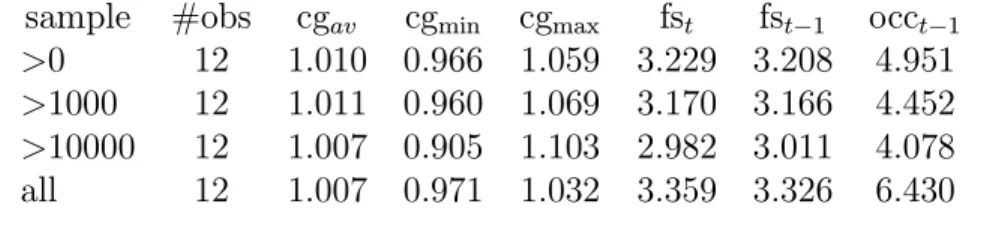
Figure 8 relates the analysis of this paper to Mankiw and Zeldes (1991). Mankiw and Zeldes (1991) were the ¯rst to emphasize the importance of asset market participation for the equity premium puzzle and for estimates of the rate of risk aversion. They also use PSID data but instead of using individual data or cohort data, they create a representative consumer for di®erent samples of consumers based on assetholdings. The representative consumer in their study is formed by ¯rst computing the average consumption level, and subsequently computing consumption growth. They ¯nd that the implied rate of risk aversion is smaller when considering assetholders and decreases when considering consumers that hold larger amounts of assets. While the analysis used in Figure 8 is slightly di®erent from Mankiw and Zeldes' approach15, the empirical results are quite similar.16 When considering samples of assetholders, the implied rate of risk aversion is smaller compared to samples that contain assetholders as well as non-assetholders. This is especially the case for ¯gure 8C as compared
of this data issue on the results, the analysis was repeated for the larger samples by repeatedly drawing subsamples with a number of observations equal to that of the smaller samples. By using these subsamples to generate similar ¯gures, I investigated how much of the di®erence in results between di®erent panels is due to di®erences in cohort size. On average, 10 to 15 % of the di®erences in risk aversion found are due to these sample size e®ects, while the remaining 85 to 90% is due to genuine di®erences in the characteristics of the di®erent types of assetholders.
14The empirical results in panels A, B and C for ¯gures 4 through 7 indicate that cohort construction in°uences estimates of the rate of risk aversion. This is not surprising given the di®erences in the descriptive statistics evidenced in tables III and IV. First, when averaging over consumption growth (in ¯gures 5 and 7), we obtain larger estimates of risk aversion compared to when averaging over the consumption level (in ¯gures 4 and 6). Also, risk aversion is a bit higher when using cohorts based on age and education (in ¯gures 4 and 5) compared to the cohorts based on age in ¯gures 6 and 7. Altogether, the ¯ndings in panels A, B and C are surprisingly robust to cohort construction.
15Mankiw and Zeldes (1991) use a local normality argument based on the continuous time model. As a result, the only determinant of the equity premium is the covariance between consumption growth and the risky return. In this study all moments of the distribution are taken into consideration.
to ¯gure 8D, and to a lesser extent for ¯gure 8B as compared to ¯gure 8D. Note also that the use of panel data in itself does not lead to lower estimates of the rate of risk aversion. The estimates of risk aversion in ¯gure 8D are in some cases higher than in Figure 1. This ¯nding is also similar to the one in Mankiw and Zeldes (1991).
4.6
Conditional Information
Figures 9, 10 and 11 discuss the role of conditional information. Whereas this is not the main focus of this paper, the graphical analysis conducted here provides some interesting perspec-tives on this issue. In the representative agent literature, the analysis of the unconditional Euler equation points towards large risk aversion but econometric analysis of the conditional Euler equation indicates small risk aversion (see Hansen and Singleton (1982)).17 However, for the individual household data the evidence seems much more robust, because the uncon-ditional Euler equation analyzed here points towards intuitively plausible parameter values that are very similar to those obtained in Jacobs (1999).
To resolve this issue, ¯gures 9, 10 and 11 further investigate the importance of conditional information for asset pricing in a perhaps unconventional fashion. These ¯gures investigate orthogonality conditions two at a time, where each pair is formed by using the Euler equation for the riskless and risky asset and one single instrument. This allows us in principle to determine both parameters of interest. So we proceed in exactly the same fashion as with the unconditional information. Figure 9 presents these results for the individual data, ¯gure 10 for the cohort data and ¯gure 11 for the representative agent data used by Mehra and Prescott (1985). Figures 9 and 10 both use same sample 3 (asset holdings > $1000) and the same instruments: lagged rates of return in panels A and B, and lagged unemployment rates in panel C. The unemployment rates are better instruments than lagged consumption because they perform better in the presence of measurement error. Panel D uses the lagged unemployment rates interacted with the age of the household head. For the representative agent data in ¯gure 11, ¯gure 11A uses the lagged risky return as an instrument, ¯gure 11B the lagged riskless return, ¯gure 11C lagged consumption growth and ¯gure 11D consumption growth lagged twice. Inspection of these ¯gures makes it quite clear that the impact of conditional information is minimal. The corresponding orthogonality conditions are solved for parameter combinations that are very similar to the case of unconditional information.
17The relationship between the estimates of the rate of risk aversion and the type of information used in the test was pointed out by Hansen and Singleton (1983) and Grossman, Melino and Shiller (1987). The issue is addressed in more detail in Singleton (1990), Ferson and Harvey (1992,1993), Ferson and Constantinides (1991) and Cochrane (2001).
4.7
Identi¯cation Problems
Finally, ¯gure 12 presents more evidence that is useful to reconcile the results in this paper with existing results in the literature. Speci¯cally, the results in ¯gures 2 and 9 indicate that individual household data always imply fairly low values of the rate of relative risk aversion. When inspecting ¯gures 1 and 11, it seems that representative agent data always lead to high estimates of the rate of risk aversion. However, several studies in the representative agent literature starting with Hansen and Singleton (1982) have obtained low estimates of the rate of risk aversion when using conditional information.
This ¯nding is due to an identi¯cation problem that is illustrated in ¯gure 12. Figure 12A is a more complete representation of the information in ¯gure 1C. It indicates that for many plausible values of ¯ (for instance ¯ =0.85), the Euler equation is solved by a rate of risk aversion in the concave region of the parameter space but also by another rate of relative risk aversion in the nonconcave region of the parameter space. The solution in the nonconcave region of the parameter space is not represented in ¯gure 1C. However, ¯gure 12A also illustrates that for very large values of the discount rate, we can have two solutions to each Euler equation that are in the concave region of the parameter space, the implausibly large one that is presented in ¯gure 1C and another value that is much smaller. Note that these smaller risk aversion values do not exactly solve the equity premium puzzle (the curve formed by joining the plus signs stays above the curve formed by joining the stars). However, those solutions ensure that the representative agent literature does not have an \equity return puzzle", which would exist using exclusively the evidence in ¯gure 1C. In ¯gure 12A, we can ¯nd discount rates smaller than 1 and low rates of risk aversion that explain the return on the risky asset by itself.
Moreover, ¯gure 12A also indicates that if we do not take into account the equity premium puzzle, the risk free rate puzzle does not exist. There are some combinations of discount rates less than one and low risk aversion that explain the riskfree rate. This is also noted for instance by Kocherlakota (1996), in his discussion of table 2 in that paper. However, the number of parameter combinations that solves the riskfree rate puzzle is much smaller than those that explain the rate of return on equity. What is perhaps not well articulated in the representative agent literature is that these parameter values that solve individual Euler equations are in a loose sense \closer" in the parameter space to parameter combinations in the nonconcave region of the parameter space (squares and triangles) than to those parameter values that are more commonly associated with asset pricing puzzles (plus signs and stars). Figure 12B illustrates that when incorporating conditional information, the evidence looks very similar to ¯gure 12A. For many plausible values of the rate of time preference, there are two rates of risk aversion in the concave region that solve the Euler equation. This is not the case when considering individual household data (or cohort data). As in the representative agent case, there is a range of discount rates for which there are two rates of risk aversion that solve the Euler equation. However, using household data it is always the
case that one rate of risk aversion is in the concave region of the parameter space and the other is not. Therefore, since the nonconcave region of the parameter space is thought of as entirely implausible, the nonconcave solution is of no interest for econometric inference.18 For the representative agent case, it is possible that certain combinations of instruments indicate a large rate of risk aversion and other combinations of instruments indicate a small rate of risk aversion, as is the case in Hansen and Singleton (1982).19
5
Conclusion
This paper demonstrates that the incomplete markets setting holds great promise to resolve a number of important issues in asset pricing, such as the equity premium puzzle and the riskfree rate puzzle. Even though no parameter combination can be found for which the Euler equation error for the riskless asset and the Euler equation error for the risky asset are both exactly zero, there exist a number of intuitively plausible combinations of the discount rate and the rate of relative risk aversion for which Euler equation errors are not statisti-cally di®erent from zero. In the representative agent literature, we can also ¯nd parameter combinations that yield Euler equation errors that are statistically indistinguishable from zero. However, these parameter combinations all imply high rates of relative risk aversion, and are therefore judged implausible.
One of the potential problems with tests of incomplete markets is the presence of substan-tial measurement error. This study investigates if the ¯ndings on the rate of risk aversion are robust to the measurement error problem by repeating the empirical tests for synthetic cohorts. While the rate of risk aversion implied by the Euler equations is a®ected, indicating that measurement error is important, the level of risk aversion is still intuitively plausible for assetholders.
These ¯ndings complement a number of ¯ndings in the existing literature on incomplete markets that are typically obtained using simulation techniques. The conclusion from this literature is that the existence of uninsurable risk can bring predicted asset returns more in line with the data, but often at the cost of employing a model economy which may be at odds with other stylized facts. For instance, the degree of persistence in shocks to
18Some authors advocate to exclude the nonconcave region of the parameter space from consideration (see Braun, Constantinides and Ferson (1993)).
19This discussion is meant to illustrate an identi¯cation problem which is not always elaborated upon in the literature. It does not claim to provide intuition for the underlying economic determinants of this identi¯cation problem. Ferson and Constantinides (1991) provide an intuitive explanation of the con°icting evidence on risk aversion in representative agent models, by associating conditional information with intertemporal substitution and the high rate of risk aversion based on unconditional information with the agent's attitude towards risk.