HAL Id: hal-03001934
https://hal.archives-ouvertes.fr/hal-03001934
Submitted on 12 Nov 2020
HAL is a multi-disciplinary open access
archive for the deposit and dissemination of sci-entific research documents, whether they are pub-lished or not. The documents may come from teaching and research institutions in France or abroad, or from public or private research centers.
L’archive ouverte pluridisciplinaire HAL, est destinée au dépôt et à la diffusion de documents scientifiques de niveau recherche, publiés ou non, émanant des établissements d’enseignement et de recherche français ou étrangers, des laboratoires publics ou privés.
Modelling of insulation in DC systems: the challenges
for HVDC cables and accessories
Thi Thu Nga Vu, G. Teyssedre
To cite this version:
Thi Thu Nga Vu, G. Teyssedre. Modelling of insulation in DC systems: the challenges for HVDC cables and accessories. Vietnam Journal of Science, Technology and Engineering, 2020, 62 (3), pp.38-44. �10.31276/VJSTE.62(3).38-44�. �hal-03001934�
Modelling of insulation in DC systems:
the challenges for HVDC cables and accessories
Vu Thi Thu Nga*, Gilbert Teyssedre21Electric Power University, Hanoi, Vietnam 2Laplace, CNRS and University of Toulouse, France
Abstract:
Cable technologies have evolved in different ways for applications using high voltage alternating current (HVAC) and high voltage direct current (HVDC) over the last 40 years. Since the 1950s, mass-impregnated paper was progressively replaced by extruded insulation made of polyethylene and then cross-linked polyethylene (XLPE). The switch from paper insulation to extruded cables went on continuously while cables were designed with ever increasing voltage requirements. However, regarding space charge build-up and field redistribution, particularly at polarity reversal stages in thyristors, the behaviour of extruded cables under such DC stress is not fully understood. For this reason, material improvement, characterization, and modelling are still intensively researched for cables, accessories, and power conversion equipment. The weaknesses and methods used to simulate the characteristics of insulation are presented and compared in this work through the simulation results of the macroscopic and fluid model.
Introduction
HVDC technologies remain a growing part of energy transmission systems owing to the new sources of energy being introduced, especially renewable energy, and to the need for strengthening energy networks while focusing on the de-carbonation of energy.
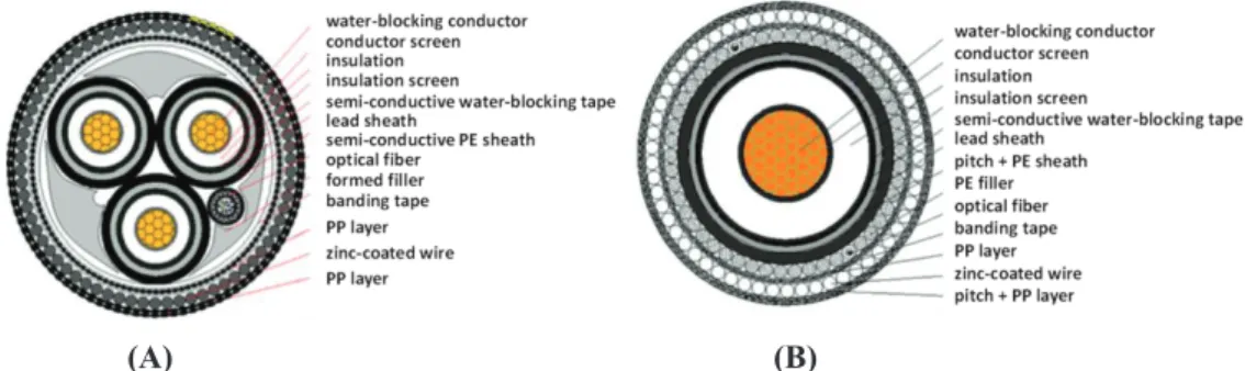
There are converging favourable conditions for the development of HVDC links for energy transmission, notably the development of large electrical power lines over long distances to link production and consumption areas and to interconnect different networks with ever growing size. HVDC can also be used in replacement of HVAC lines for transmitting more power over a spatially constrained infrastructure. The demand for HVDC lines has diverse origins, namely, submarine cables, urban areas, and strong public opposition of overhead lines. The switch from HVAC to HVDC systems has great advantages such as simplification of manufacture (Fig. 1) and virtually no limit on transmission length owing to the fact that compensation of the capacitive current is no longer a necessity. Therefore, materials used for the insulation of HVDC cables require specific properties, notably regarding conductivity behaviour. Aside from that, its space charge behaviour is something that is carefully considered at the material characterization level (as samples), as well as in a full cable configuration. The amount of charges is something that can be relatively well characterized, however, the criteria for the kinetics of charge release and the behaviour of materials at polarity reversal are not so well-defined [1]. A slow relaxation of charges implies that, at polarity reversal, the residual field will add to the applied field. Therefore, the objective of this work is the analysis of the weaknesses and methods used to simulate the characteristics of insulation in cables and accessories under DC electro-thermal stress.
Threats for insulation withstanding in HVDC cables
As mentioned above, one of the threats to insulation under HVDC stress is the build-up of space charges in the insulation and its impact on the field distribution, along with the energy released when charges are redistributed upon fast-varying voltage. The weaknesses of polymers with respect to mass-impregnated paper can be found in their lower thermal conductivity and higher electrical resistivity, such that charge release is slower. For example, in mineral insulated (Mi) cables, trapped space charge accumulation is considered insignificant [3]. Also, the maximal designed thermal stress is 55°C for Mi-paper while it is 90°C for XLPE, at least under AC stress.
The major difference between HVAC and HVDC stress is the change from a capacitive distribution of the field to a resistive distribution; as even under DC there is a progressive switch from capacitive to resistive field distribution at each stress level. Under operating conditions, the electric field is not homogeneous along the cable radius and a thermal gradient exists along the radius due Joule losses from the circulating current in the conductor. As the resistivity of the insulation is much more dependent on the temperature and electric field than it is the permittivity, the thermal-electric stress rating in an HVDC cable is trickier to achieve. Under steady-state HVDC, the phenomenon of stress inversion occurs; i.e. the electric field becomes higher at the outer semiconducting screen than at the inner one (near the conductor) due to the lower temperature. Hence, lower electrical conductivity is found at the outer screen. An example of such stress inversion is represented in Fig. 2 for a medium voltage cable under a thermal gradient of 30°C as modelled by a realistic law for the electric conductivity of polyethylene insulation [4] given by:
3
redistributed upon fast-varying voltage. The weaknesses of polymers with respect to mass-impregnated paper can be found in their lower thermal conductivity and higher electrical resistivity, such that charge release is slower. For example, in mineral insulated (Mi) cables, trapped space charge accumulation is considered insignificant [3]. Also, the maximal designed thermal stress is 55°C for Mi-paper while it is 90°C for XLPE, at least under AC stress.
The major difference between HVAC and HVDC stress is the change from a capacitive distribution of the field to a resistive distribution; as even under DC there is a progressive switch from capacitive to resistive field distribution at each stress level. Under operating conditions, the electric field is not homogeneous along the cable radius and a thermal gradient exists along the radius due Joule losses from the circulating current in the conductor. As the resistivity of the insulation is much more dependent on the temperature and electric field than it is the permittivity, the thermal-electric stress rating in an HVDC cable is trickier to achieve. Under steady-state HVDC, the phenomenon of stress inversion occurs; i.e. the electric field becomes higher at the outer semiconducting screen than at the inner one (near the conductor) due to the lower temperature. Hence, lower electrical conductivity is found at the outer screen. An example of such stress inversion is represented in Fig. 2 for a medium voltage cable under a thermal gradient of 30°C as modelled by a realistic law for the electric conductivity of polyethylene insulation [4] given by:
( ) ( ) ( ( ) ) (1) where A and α are constants, Ea is the thermal activation energy, kB is
Boltzmann’s constant, E is the applied electric field, T is the temperature, and B = aT+b is a temperature-dependent parameter to account for the change in threshold field versus temperature. it can be seen that the field initially exhibits a capacitive distribution; after 1000 s it is relatively homogeneous and after 1 h or so, the field is a maximum at the outer shield. The switch from capacitive to resistive field distribution is controlled by the dielectric time constant, ε/σ, where ε is the dielectric permittivity. When the polarity is reversed, which is usually done over a time much faster than the dielectric time constant, the residual electric field at the inner conductor
(1) where A and α are constants, Ea is the thermal activation energy, kB is Boltzmann’s constant, E is the applied electric
field, T is the temperature, and B = aT+b is a temperature-dependent parameter to account for the change in threshold field versus temperature. It can be seen that the field initially exhibits a capacitive distribution; after 1000 s it is relatively homogeneous and after 1 h or so, the field is a maximum at the outer shield. The switch from capacitive to resistive field distribution is controlled by the dielectric time constant, ε/σ, where ε is the dielectric permittivity. When the polarity is reversed, which is usually done over a time much faster than the dielectric time constant, the residual electric field at the inner conductor constitutes an enhancement to the capacitive field and this local and transient enhancement of the field brings harmfulness to the cables.
Fig. 2. Example of field redistribution vs. time and stress inversion under DC stress for a MV cable. Adapted from [5].
parameters of equation (1) are: A=3.68×10⁷ S•m/V, E
a=0.98 eV,
B=1.086×10⁻⁷ S•m/V and α=1. A temperature drop of 30°C across
the insulator and a temperature of 80oC at the inner conductor
are considered.
From the assumption on the temperature dependence of conductivity, using Maxwell’s equation, it can be shown that the electric field distribution in the cable insulation, in cylindrical geometry and under steady state condition is given by expression [6, 7]:
2
(A) (B)
Fig. 1. Examples of structures of HV submarine cables rated for 200 MW. Weight reduced by over 60% [2]. (A) 3-core HVAC 110 kV cable; outer diameter 193 mm; (B)
+/- 160 kV HVDC cable; outer diameter 111 mm.
consumption areas and to interconnect different networks with ever
growing size. HVDC can also be used in replacement of HVAC lines for
transmitting more power over a spatially constrained infrastructure. The
demand for HVDC lines has diverse origins, namely, submarine cables,
urban areas, and strong public opposition of overhead lines. The switch
from HVAC to HVDC systems has great advantages such as simplification
of manufacture (Fig. 1) and virtually no limit on transmission length owing
to the fact that compensation of the capacitive current is no longer a
necessity. Therefore, materials used for the insulation of HVDC cables
require specific properties, notably regarding conductivity behaviour. Aside
from that, its space charge behaviour is something that is carefully
considered at the material characterization level (as samples), as well as in a
full cable configuration. The amount of charges is something that can be
relatively well characterized, however, the criteria for the kinetics of charge
release and the behaviour of materials at polarity reversal are not so
well-defined [1]. A slow relaxation of charges implies that, at polarity reversal,
the residual field will add to the applied field. Therefore, the objective of
this work is the analysis of the weaknesses and methods used to simulate
the characteristics of insulation in cables and accessories under DC
electro-thermal stress.
Threats for insulation withstanding in HVDC cables
As mentioned above, one of the threats to insulation under HVDC
stress is the build-up of space charges in the insulation and its impact on the
field distribution, along with the energy released when charges are
(A) (B)Fig. 1. Examples of structures of HV submarine cables rated for 200 MW. Weight reduced by over 60% [2]. (A) 3-core HVAC 110
4
constitutes an enhancement to the capacitive field and this local and
transient enhancement of the field brings harmfulness to the cables.
Fig. 2. Example of field redistribution vs. time and stress inversion under DC stress for a MV cable. Adapted from [5]. Parameters of equation (1) are: A=3.68107 S•m/V, Ea=0.98 eV, B=1.08610-7 S•m/V and α=1. A temperature drop of 30°C across the insulator and a temperature of 80°C at the inner conductor are considered.
From the assumption on the temperature dependence of conductivity,
using Maxwell's equation, it can be shown that the electric field distribution
in the cable insulation, in cylindrical geometry and under steady state
condition is given by expression [6, 7]:
( )
( )(2)
where E
0and
0are, respectively, the electric field and conductivity at the
reference position, r
0. The charge density associated with non-uniform
conductivity is of the form:
(3)
where
is the dielectric permittivity of the material. if the temperature
dependence of the conductivity follows the Arrhenius law with activation
energy E
a, the charge density can be written according to the following
equation:
dr
r r r E E div r g ( ) ( ) (2) where E0 and σ0 are, respectively, the electric field and conductivity at the reference position, r0. The charge density associated with non-uniform conductivity is of the form:4
constitutes an enhancement to the capacitive field and this local and
transient enhancement of the field brings harmfulness to the cables.
Fig. 2. Example of field redistribution vs. time and stress inversion under DC stress for a MV cable. Adapted from [5]. Parameters of equation (1) are: A=3.68107 S•m/V, Ea=0.98 eV, B=1.08610-7 S•m/V and α=1. A temperature drop of 30°C across the insulator and a temperature of 80°C at the inner conductor are considered.
From the assumption on the temperature dependence of conductivity,
using Maxwell's equation, it can be shown that the electric field distribution
in the cable insulation, in cylindrical geometry and under steady state
condition is given by expression [6, 7]:
( )
( )(2)
where E
0and
0are, respectively, the electric field and conductivity at the
reference position, r
0. The charge density associated with non-uniform
conductivity is of the form:
(3)
where
is the dielectric permittivity of the material. if the temperature
dependence of the conductivity follows the Arrhenius law with activation
energy E
a, the charge density can be written according to the following
equation:
dr
r r r E E div r g ( ) ( ) (3)where ε is the dielectric permittivity of the material. if the temperature dependence of the conductivity follows the Arrhenius law with activation energy Ea, the charge density can be written according to the following equation:
5
( ) ( )
,
(4)
where T is the absolute temperature, which is function of r and time, t [8]. it
can be noticed from Eqs. (3) and (4) that the space charge polarity directly
depends on the conductivity gradient d
/dr.
The sign of the space charge, ρ
g(r), is the same as the polarity of the
voltage applied to the conductor. Such space charge is normally detected by
experimental techniques that provide the charge distributions. Such a
geometric space charge is also detected when dielectrics of different natures
become associated, as in joints and terminations of cables. These junctions
may correspond to a gradient of permittivity, or more likely, to a gradient of
conductivity [9, 10]. We have shown that such an interfacial charge - or
macroscopic Maxwell-Wagner effect - can be probed by the space charge
measurement method. Depending on temperature and field values, the field
can be a maximum in one or the other dielectric. Also, the kinetics for
build-up and release of the interface charge depends on field and
temperature [11].
Besides these geometric space charge effects there are also processes of
charge build up due to charge trapping and internal dissociation
phenomena. it was shown that the latter effect is strongly influenced by the
presence of crosslinking by-products into cross-linked polyethylene.
Progress in material behaviour when going from HVAC grade to HVDC
was obtained by lowering the amount of crosslinking by-products or even
suppressing them completely. But still, the issue remains where electronic
carriers can be deeply trapped in the material and contribute to field
distortion. There is a general trend towards using high resistivity materials
[12] to avoid notable thermal runaway and possible breakdown in the cable
[5]. However, this may be accompanied with slower space charge release.
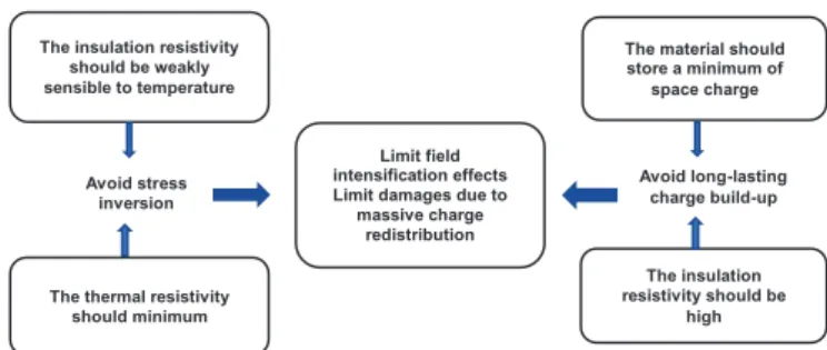
So, a kind of trade off has to be found. Figure 3 provides some desired
features for insulations with an aim to avoid stress enhancement and heavy
charge redistribution, of which both processes lead to damages.
(4) where T is the absolute temperature, which is function of r and time, t [8]. it can be noticed from Eqs. (3) and (4) that the space charge polarity directly depends on the conductivity gradient dσ/dr.
The sign of the space charge, ρg(r), is the same as the
polarity of the voltage applied to the conductor. Such space charge is normally detected by experimental techniques that provide the charge distributions. Such a geometric space charge is also detected when dielectrics of different natures become associated, as in joints and terminations of cables. These junctions may correspond to a gradient of permittivity, or more likely, to a gradient of conductivity [9, 10]. We have shown that such an interfacial charge - or macroscopic Maxwell-Wagner effect - can be probed by the space charge measurement method. Depending on temperature and field values, the field can be a maximum in one or the other dielectric. Also, the kinetics for build-up and release of the interface charge depends on field and temperature [11].
Besides these geometric space charge effects there are also processes of charge build up due to charge trapping and internal dissociation phenomena. it was shown that the latter effect is strongly influenced by the presence of crosslinking by-products into cross-linked polyethylene. Progress in material behaviour when going from HVAC grade to HVDC was obtained by lowering the amount of crosslinking by-products or even suppressing them completely. But still, the issue remains where electronic carriers can be deeply trapped in the material and contribute to field distortion. There is a general trend towards using high resistivity materials [12] to avoid notable thermal runaway and possible breakdown in the cable [5]. However, this may be accompanied with slower space charge release. So, a kind of trade off has to be found. Fig 3 provides some desired features for insulations with an aim to avoid stress enhancement and heavy charge redistribution, of which both processes lead to damages.
6
Fig. 3. Strategies for improving material withstanding in HVDC.
Thermal resistivity should be minimized to limit thermal gradients, the insulation’s resistivity should be comparatively insensitive to temperature, and having nonlinear properties is attractive for field homogenization purposes (as with paper-oil insulation). These three conditions should limit field intensification. one way to avoid heavy charge distribution is to prevent charge storage, and another is to increase resistivity. However, a higher resistivity can also favour persistent charge storage. Therefore, at the same time as resistivity is reduced, charge generation processes should be avoided. Last, but not least, the DC breakdown stress should be high, even at high temperature, and the material should be insensitive to polarity reversal.
Modelling of insulations under dc electro-thermal stress
Several models have been proposed in the literature through the years to predict space charge and electric field distribution within an insulating material subjected to DC electro-thermal stress. Among these models, two types have been extensively used for the materials of HVDC systems, namely, macroscopic models and fluid models. These models will be described in the following paragraphs and simulation results will be presented for each model and for relevant cases linked to HVDC cables and accessories.
Macroscopic models
The material is considered as weakly conductive for these models and only a gradient in the applied stress (electric field, temperature, etc.) in the material will induce the appearance of a space charge due to non-homogeneity of the conductivity. These models have the advantage of
The insulation resistivity should be
high The insulation resistivity
should be weakly sensible to temperature
The thermal resistivity should minimum
Avoid stress inversion
The material should store a minimum of space charge Avoid long-lasting charge build-up Limit field intensification effects Limit damages due to massive charge
redistribution
Fig. 3. Strategies for improving material withstanding in HVDC.
Thermal resistivity should be minimized to limit thermal gradients, the insulation’s resistivity should be comparatively insensitive to temperature, and having nonlinear properties is attractive for field homogenization purposes (as with paper-oil insulation). These three conditions should limit field intensification. One way to avoid heavy charge distribution is to prevent charge storage, and another is to increase resistivity. However, a higher resistivity can also favour persistent charge storage. Therefore, at the same time as resistivity is reduced, charge generation processes should be avoided. Last, but not least, the DC breakdown stress should be high, even at high temperature, and the material should be insensitive to polarity reversal.
Modelling of insulations under DC electro-thermal stress
Several models have been proposed in the literature through the years to predict space charge and electric field distribution within an insulating material subjected to DC electro-thermal stress. Among these models, two types have been extensively used for the materials of HVDC systems, namely, macroscopic models and fluid models. These models will be described in the following paragraphs and simulation results will be presented for each model and for relevant cases linked to HVDC cables and accessories.
Macroscopic models
The material is considered as weakly conductive for these models and only a gradient in the applied stress (electric field, temperature, etc.) in the material will induce the appearance of a space charge due to non-homogeneity of the conductivity. These models have the advantage of requiring only a few macroscopic parameters, namely, conductivity and permittivity, to simulate the electric field distribution in an insulator. While conductivity is a non-linear function of the electric field and temperature, it is relatively easy to measure experimentally. This has been done for XLPE at different fields and temperatures [10] and an equation for the conductivity variation as a function of these parameters has also been proposed (Eq. 1) [10, 13]. With these data, it is possible to simulate the field and space charge dynamics in a loaded cable with a conductivity gradient. An example of such a calculation is proposed in Fig. 4 for an XLPE-insulated medium voltage (MV) cable 4.5 mm thick, under
7
requiring only a few macroscopic parameters, namely, conductivity and
permittivity, to simulate the electric field distribution in an insulator. While
conductivity is a non-linear function of the electric field and temperature, it
is relatively easy to measure experimentally. This has been done for XLPE
at different fields and temperatures [10] and an equation for the
conductivity variation as a function of these parameters has also been
proposed (Eq. 1) [10, 13]. With these data, it is possible to simulate the
field and space charge dynamics in a loaded cable with a conductivity
gradient. An example of such a calculation is proposed in Fig. 4 for an
XLPE-insulated medium voltage (MV) cable 4.5 mm thick, under an
applied voltage of -80 kV, and a temperature gradient of ΔT=16°C (i.e.
T
in=57°C and T
out=41°C) across the insulation.
(A) (B)
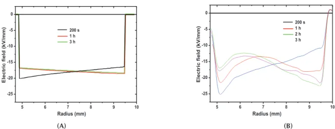
Fig. 4. Field distributions at different times for an MV cable under -80 kV and
temperature gradient of ΔT=16°C. (A) Calculated (macroscopic model), (B) Measured
by pulsed-electro acoustic (PEA) method.
The details concerning the conductivity equation, the protocol, and the
numerical calculations are detailed elsewhere [10]. The experimental fields
calculated from space charge measurements using the pulsed electro
acoustic (PEA) method are given in Fig. 4B for comparison (the electric
field should start at 0 but this part of the inner conductor is not visible due
to the method used). In the simulation, the field distribution quickly
deviates from the Laplacian field and achieves a maximum of the electric
field at the outer electrode after one hour of polarization. The field
distribution stabilizes with time. The maximal electric field values
calculated are, respectively, 17 and 18.5 kV/mm at the inner and outer
5 6 7 8 9 10 -25 -20 -15 -10 -5 0 El ec tr ic fie ld (k V/mm ) Radius (mm) 200 s 1 h 2 h 3 h 7
requiring only a few macroscopic parameters, namely, conductivity and
permittivity, to simulate the electric field distribution in an insulator. While
conductivity is a non-linear function of the electric field and temperature, it
is relatively easy to measure experimentally. This has been done for XLPE
at different fields and temperatures [10] and an equation for the
conductivity variation as a function of these parameters has also been
proposed (Eq. 1) [10, 13]. With these data, it is possible to simulate the
field and space charge dynamics in a loaded cable with a conductivity
gradient. An example of such a calculation is proposed in Fig. 4 for an
XLPE-insulated medium voltage (MV) cable 4.5 mm thick, under an
applied voltage of -80 kV, and a temperature gradient of ΔT=16°C (i.e.
T
in=57°C and T
out=41°C) across the insulation.
(A) (B)
Fig. 4. Field distributions at different times for an MV cable under -80 kV and
temperature gradient of ΔT=16°C. (A) Calculated (macroscopic model), (B) Measured
by pulsed-electro acoustic (PEA) method.
The details concerning the conductivity equation, the protocol, and the
numerical calculations are detailed elsewhere [10]. The experimental fields
calculated from space charge measurements using the pulsed electro
acoustic (PEA) method are given in Fig. 4B for comparison (the electric
field should start at 0 but this part of the inner conductor is not visible due
to the method used). In the simulation, the field distribution quickly
deviates from the Laplacian field and achieves a maximum of the electric
field at the outer electrode after one hour of polarization. The field
distribution stabilizes with time. The maximal electric field values
calculated are, respectively, 17 and 18.5 kV/mm at the inner and outer
5 6 7 8 9 10 -25 -20 -15 -10 -5 0 El ec tr ic fie ld (k V/mm ) Radius (mm) 200 s 1 h 3 h
an applied voltage of -80 kV, and a temperature gradient of ΔT=16°C (i.e. Tin=57°C and Tout=41°C) across the insulation.
The details concerning the conductivity equation, the protocol, and the numerical calculations are detailed elsewhere [10]. The experimental fields calculated from space charge measurements using the pulsed electro acoustic (PEA) method are given in Fig. 4B for comparison (the electric field should start at 0 but this part of the inner conductor is not visible due to the method used). in the simulation, the field distribution quickly deviates from the Laplacian field and achieves a maximum of the electric field at the outer electrode after one hour of polarization. The field distribution stabilizes with time. The maximal electric field values calculated are, respectively, 17 and 18.5 kV/mm at the inner and outer semiconductor. This change from capacitive (i.e. Laplacian field) to a resistive field distribution is due to the conductivity gradient that drives charges from the higher conductivity (inner semiconductor) to the lower conductivity (outer semiconductor). When compared to the experimental data, the same trend is observed, i.e. an inversion of the location of the maximal value of the electric field after one hour. However, in the experiment, the value is twice that which has been predicted by the macroscopic model (~20 kV/mm at the outer semiconductor). Hence, the macroscopic model can only predict the field values under the limits fixed by the conductivity variation linked to the thermal and/or electrical gradient. if other physical phenomena are at play in the cable, these types of models
are not sufficient to predict the entire field response. The real advantage of such a macroscopic model is to use it for large systems, where often times complex geometries and a large number of materials are present, to provide the field distribution along the system. This is, for example, the case with HVDC cable joints where different dielectrics are used and where the geometry plays a key role in the field pattern. Fig 5 shows an example of a pre-moulded joint actually used for a 200 kV DC link, where an interface is formed between two insulating polymers, namely XLPE and ethylene propylene diene monomer (EPDM). This geometry has been implemented in the macroscopic model. Under the simulation conditions, a voltage of 200 kV is applied at the inner side of the XLPE and the outer face of the EPDM is grounded. A current of I=1000 A flows in the conductor core. These conditions imply a temperature gradient as well as a field gradient, in the cable joint.
The calculated electric field distribution in the cable joint is presented in Fig. 6, for the proposed geometry of Fig. 5. in the simulations, we consider here that the thermal and electrical conditions have reached stationary states, with a thermal gradient on the order of 40°C between the cable core and the outside of the joint. The maximal values of the electric field are located, respectively, at the triple point of the XLPE, EPDM, semiconductor, and at the XLPE/EPDM interface at the limit of the cable joint. The field distribution in these regions is controlled by stress cones. The design and modelling of these parts actually represent one of the key points for reliable cable accessories [5, 15-17].
5 6 7 8 9 10 -25 -20 -15 -10 -5 0 El ec tr ic fie ld (k V/mm ) Radius (mm) 200 s 1 h 3 h 5 6 7 8 9 10 -25 -20 -15 -10 -5 0 El ec tr ic fie ld (k V/mm ) Radius (mm) 200 s 1 h 2 h 3 h (A) (B)
Fig. 4. Field distributions at different times for an MV cable under -80 kV and temperature gradient of ΔT=16°C. (A) Calculated
42
Fig. 5. Schematic representation of a pre-moulded joint for HVDC-extruded cables up to 200 kV [14].
Fig.6. Electric field distribution ina cable jointunder Vappl=200 kV and I=1000 A. the colour scale implies a high electric field for
red colours, and a lower electric field for blue colours.
This example shows the necessity to optimize the various parameters that play a role in the electric field distribution in cable joints, such as the system geometry (at the triple point but also at the junction boundary) and the material properties. Macroscopic modelling could be used as a design tool to optimize these parameters in regard to temperature and field with the goal of developing new materials with specific properties.
Fluid models
Contrary to macroscopic models, fluid models are based on a microscopic approach, where the physical hypotheses at play should be identified before any model development.
They do not rely on the non-homogeneity of the conductivity, but on the generation and transport/accumulation of charges within the material. instead of considering the conductivity as a macroscopic and homogeneous phenomenon under isotropic conditions, the location where charges are generated is taken into account, as well as their nature and fate during transport. These models can simulate the transient processes that occur when a thermo-electrical stress is applied to an insulating polymer. They account for processes linked to the energy levels located in the band gap, i.e. traps for electrons and holes. They also account for charge generation and extraction at the electrodes. These models are more difficult to implement compared to macroscopic models due to the parameterization of the traps distribution. However, as charge transport is linked to trapping and detrapping, charge accumulation can take place for reasons that are not linked to the non-homogeneity of the conductivity, for example, as a blocking contact at an interface.
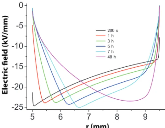
Fluid models have been intensively developed these last 20 years [18-20], mostly for low density polyethylene (LDPE), the base resin of XLPE. An example of simulation results using a fluid model for an XLPE cable is proposed
43
Elec
tric field (kV/mm)
r (mm)
Fig. 7. Simulated electric field distribution (fluid model) vs. radius at different times for an MV cable of 4.5 mm thick insulation polarized at -80 kV, and a temperature gradient of ΔT=16°C.
in Fig. 7, for the same protocol as the one described for the macroscopic model, i.e. an MV cable of 4.5 mm, an applied voltage of -80 kV, and a temperature gradient of 16°C with same internal and external temperatures as mentioned previously. The charges that are accounted for are electronic charges, i.e. electrons and holes. These charges are generated only at the electrodes and follow the Schottky injection law. Charges can be mobile, having a hopping mobility that is a function of the electric field and temperature, or charges can be trapped into a unique level of deep traps, from which they can escape by a thermally activated process. Recombination is also taken into account in the fluid models. Recombination coefficients between each type of charge are a function of the mobility (i.e. Langevin coefficients). A complete description of the physical hypotheses included in the model, the numerical resolution, and the parameterization are detailed elsewhere for cable geometry [21]. When considering the simulated results at a steady state (i.e. 48 h), the electric field distribution is seen to switch from the Laplace field to its maximal value at the outer semiconductor. Moreover, the maximal field value at the outer electrode is on the order of 22.5 kV/mm, which is what has been measured experimentally. From these results, it is noticeable that the fluid model can predict the main characteristics observed experimentally, particularly the field enhancement at the outer electrode compared to the macroscopic model, which is not only due to a conductivity gradient. However, for these models, different processes are at play, with various characteristic times for each process. in this case, the parameterization is very sensitive and has not
reached an optimized point and, in the proposed example, the dynamics for field stabilization is longer (48 h) compared to the experimental case (3 h).
Comparing fluid models to macroscopic models by means of electric field distribution shows the strengths and drawbacks of each model:
- Macroscopic models offer an easy implementation of the conductivity and the possibility to simulate complex systems over short time simulations. They are, however, limited when charge accumulation comes into play.
- Fluid models possess an efficient description of the charge behaviour, but at the cost of complex physics and parameterization. Aside from their direct implementation in real geometries in which parameterization and optimization are tricky, fluid models are interesting and efficient for testing hypotheses of physical processes controlling the charging behaviour. Such models are developed based on focused experiments that can be realized at a lab scale, as with electron beam irradiation.
Conclusions
According to current trends, HVDC cables are gradually replacing HVAC because of their significant benefits. However, due to the build-up of space charge and the consequent distortion electric fields, the challenge of designing insulating materials under DC stress is not straightforward. We have explored various research directions for the development of insulating materials and control of stresses upon DC cables by simulations and modelling using different methods. The simulation results of the macroscopic models and fluid models are compared in this work. The macroscopic models have the ability to simulate complex systems over a short time, however, the model is affected by the formation of space charges in the material. Fluid models are effective in modelling the physical processes that control the charging behaviour, but they are difficult in real geometries due to complex parameterization and optimization.
ACKNOWLEDGEMENTS
We would like to acknowledge the C.N.R.S. (France) for financial support to the ModHVDC project n° PICS07965.
The authors declare that there is no conflict of interest regarding the publication of this article.
44
REFERENCES
[1] T.T.N. Vu, G. Teyssedre, S. Le Roy, et al. (2017), “Space charge criteria for the assessment of insulation materials for HVDC”,
IEEE Trans. Dielectr. Electr. Insul., 24, pp.1405-1415.
[2] H.L. Zhang, J.M. Zhang, L. Duan, et al. (2017), “Application status of XLPE insulated submarine cable used in offshore wind farm
in China”, J. Eng., 13, pp.702-707.
[3] Z.Y. Huang, J.A. Pilgrim, P.L. Lewin, et al. (2015), “Thermal-electric rating method for mass-impregnated paper-insulated HVDC
cable circuits”, IEEE Trans Power Delivery, 30, pp.437-444.
[4] S. Qin, S. Boggs (2012), “Design considerations for HVDC
components”, IEEE Electr. Insul. Mag., 28(6), pp.36-44.
[5] C.o. olsson (2008), “Modelling of thermal behaviour of polymer insulation at high electric DC field”, 5th European
Thermal-Sciences Conf., pp.1-8.
[6] D. Fabiani, G.C. Montanari, C. Laurent, et al. (2008), “HVDC cable design and space charge accumulation. Part 3: Effect of
temperature gradient”, IEEE Electr. Insul. Mag., 24(2), pp.5-14.
[7] N. Adi, T.T.N. Vu, G. Teyssèdre, et al. (2017), “DC model cable under polarity inversion and thermal gradient: build-up of
design-related space charge”, Technologies, 5(46), Doi:10.3390/
technologies.
[8] G. Mazzanti, M. Marzinotto (2013), Extruded Cables for
HVDC Transmission: Advances in Research and Development, iEEE
Press-Wiley.
[9] S. Delpino, D. Fabiani, G.C. Montanari, et al. (2008), “Polymeric HVDC cable design and space charge accumulation. Part
2: insulation interfaces”, IEEE Electr. Insul. Mag., 24 (1), pp.14-24.
[10] T.T.N. Vu, G. Teyssedre, B. Vissouvanadin, et al. (2015), “Correlating conductivity and space charge measurements in multi-dielectrics under various electrical and thermal stresses”, IEEE Trans.
Dielectr. Electr. Insul., 22, pp.117-127.
[11] T.T.N. Vu, G. Teyssedre, S. Le Roy, et al. (2017), “Maxwell-Wagner effect in multi-layered dielectrics: interfacial charge
measurement and modelling”, Technologies, 5(2), Doi:10.3390/
technologies 5020027.
[12] V. Englund, J. Andersson, J.o. Boström, et al. (2014), “Characteristics of candidate material systems for next generation extruded HVDC cables”, Proc. Cigre Conference, Paris, Paper D1-104.
[13] Silec Cable, One-Piece Premolded Joint for Extruded Cables
from 63 to 500 kV.
[14] M. Jeroense, M. Saltzer, H. Gorbani (2013), “Technical challenges linked to HVDC cable development”, Proc. European
Seminar on Materials for HVDC Cables and Accessories (Jicable),
Perpignan, France, pp.1-6.
[15] D. Quaggia (2015), “Development of joints and terminations for HVDC extruded cables”, Proc. INMR-Insulator News and Market
Report, Munich, Germany, pp.228-234.
[16] S. Hou, M. Fu, C. Li, et al. (2015), “Electric field calculation and analysis of HVDC cable joints with nonlinear materials”, Proc.
IEEE 11th Internat. Conf. Properties Appl. Dielectric Materials (ICPADM), pp.184-187.
[17]. H. Ye, T. Fechner, X. Lei, et al. (2018), “Review on HVDC
cable terminations”, High Volt., 3, pp.79-89.
[18] J.M. Alison, R.M. Hill (1994), “A model for bipolar charge transport, trapping and recombination in degassed cross-linked
polyethylene”, J. Phys. D, 27, pp.1291-1299.
[19] S. Le Roy, G. Teyssedre, C. Laurent, et al. (2006), “Description of charge transport in polyethylene using a fluid model with a constant mobility: fitting model and experiments”, J. Phys. D,
39, pp.1427-1436.
[20] J. Xia, Y. Zhang, F. Zheng, et al. (2011), “Numerical analysis of packet-like charge behavior in low-density polyethylene by a Gunn
effect-like model”, J. Appl. Phys., 109, Doi: 10.1063/1.3532052.
[21] S. Le Roy, G. Teyssedre, C. Laurent (2016), “Modelling space charge in a cable geometry”, IEEE Trans. Dielectr. Electr.
![Fig. 5. Schematic representation of a pre-moulded joint for HVDC-extruded cables up to 200 kV [14]](https://thumb-eu.123doks.com/thumbv2/123doknet/14374179.504837/6.956.118.857.153.552/fig-schematic-representation-moulded-joint-hvdc-extruded-cables.webp)