System architecture and circuit design for micro and nanoresonators-based mass sensing arrays

(1)

HAL Id: tel-00658843

https://tel.archives-ouvertes.fr/tel-00658843v2

Submitted on 2 Oct 2013

HAL is a multi-disciplinary open access

archive for the deposit and dissemination of sci-entific research documents, whether they are pub-lished or not. The documents may come from teaching and research institutions in France or abroad, or from public or private research centers.

L’archive ouverte pluridisciplinaire HAL, est destinée au dépôt et à la diffusion de documents scientifiques de niveau recherche, publiés ou non, émanant des établissements d’enseignement et de recherche français ou étrangers, des laboratoires publics ou privés.

System architecture and circuit design for micro and

nanoresonators-based mass sensing arrays

Grégory Arndt

To cite this version:

Grégory Arndt. System architecture and circuit design for micro and nanoresonators-based mass sensing arrays. Other [cond-mat.other]. Université Paris Sud - Paris XI, 2011. English. �NNT : 2011PA112358�. �tel-00658843v2�

(2)

! ! ! N° d’ordre!"!#$%%&#'&()! ! !

!"#$%"&'('$

$

)!*+,-.,%/0$!1/),+)$ $ ! Ecole Doctorale « Sciences et Technologies de l’Information des$ %232456678(49:(58'$&:$;&'$)<':=6&'$>! ! ! ! !"#$# !

?@&A5@<$-BC#%$

! ! ! ! "#$%&'()! ! "*+(&,!-.'/0(&'(#.&!-12!'0.'#0(!2&+031!45.!,0'.5!-12!1-15.&+51-(5.+6$-+&2!,-++!+&1+013! -..-*+! ! ! ! ! 7&4&12&2!(/&!89!7&'&,$&.!9:88!;0(/!(/&!45<<5;013!%#.*!,&,$&.+)! ! ! !

#@$D73(&8$-@49658&! =>?6@>ABC!D01-(&'! "#E&.F0+5.! #@$C7@(9$E9@8(53! G10F&.+0(-(!?#(515,-!2&!H-.'&<51-! I-EE5.(&#.! #@$-39(8$E5''&F5&7G! G10F&.+0(J!K-.0+!88C!B>L! K.&+02&1(!54!(/&!%#.*! #@$*@(4$+53(8&:! =>?6@>ABC!D01-(&'! "#E&.F0+5.!

H6&$B5'&IH9@(&$+9J&339! Direction Générale de l’Armement! >M-,01&.! #@$!"(3(J$K&8A! =-+&!N&+(&.1!G10F&.+0(*C!>=">!L-'#<(*!! I-EE5.(&#.! #@$D2@L6&$D7(339@;! "#EJ<&'C!"">! "#E&.F0+5.!

#@$!9'493$C57&:! =OI"C!@BIDD! >M-,01&.!

!

(3)

(4)

Acknowledgments

I gratefully acknowledge the guidance provided by my director, Prof. Jérôme Juil-lard, for my entire PhD project. I always appreciated his advice and admired how available he always was even when our backgrounds and our research interests di-verged. I am also very grateful for his help and guidance during the difficult task of scientific writing. I extend my thanks to Dr. Eric Colinet, particularly for the support and the supervision during my use of the many different devices employed in the different projects. I also thank him for choosing my PhD subject, and his tolerance to my attitude which can sometimes be quite stubborn. I am particularly grateful for his vision which provided depth and substance to my PhD. Dr. Julien Arcamone and Gérard Billot guided and taught me about the fabrication process and analog design and I will always be grateful for the skills they gave me.

Towards the end of my PhD, I particularly appreciated the help provided by Julien Philippe during his internship. He has characterized many co-integrated devices and provided invaluable expertise. I also appreciated his positive attitude and thoroughly enjoyed working with him. I also acquired first-hand experience of management through our interaction. I wish him all the best in his ongoing PhD studies. I am also grateful for the time and the interesting technical discussions I had with Paul Ivaldi, Dr. Cécilia Dupré, Dr. Laurent Duraffourg, Dr. Patrick Villard, Dr. Thomas Ernst, Dr. Sébastien Hentz, Patrick Audebert, Sylvain Dumas, Dr. Guillaume Jourdan and many others. I have also appreciate the enjoyable and profitable time spent in Leti due largely to the input and friendship of Olivier Martin, Matthieu Dubois, Eric Sage, Dr. Marc Belleville, and Pierre Vincent.

I thank Prof. Nuria Barniol and Dr. Philip Feng for their time and interest towards my PhD manuscript and defense. I appreciated their constructive remarks and advice. I also thank Prof. Pascal Nouet and Prof. Alain Bosseboeuf for coming to my PhD defense and their interesting questions. I was particularly grateful that Prof. Alain Bosseboeuf accepted to be the president of the jury.

Finally, my thoughts go to my family (particularly my parents) and friends who encouraged me during my studies. I am sure I could not have finished my PhD without their support.

(5)

(6)

Abstract

This manuscript focuses on micro or nanomechanical resonators and their surround-ing readout electronics environment. Mechanical components are employed to sense masses in the attogram range (10≠18 _{g) or extremely low gas concentrations. The}

study focuses particularly on circuit architectures and on resonators that can be implemented in arrays.

In the first chapter, several architectures for tracking the resonance frequency of the mechanical structure (used to measure a mass) are compared. The two major strate-gies are frequency locked-loops and self-oscillating loops. The former is robust and versatile but is area-demanding and difficult to implement into a compact integrated circuit. Self-oscillating loops are compact but are sensitive to parasitic signals and nonlinearity. This architecture was chosen as the focus of the PhD project because of its compactness, which is necessary for the employment of arrays of sensors. In the second chapter, the electromechanical response of a sensor composed of a me-chanical resonator and an appropriate electronics is assessed. Four resonators were chosen for mass spectrometry on the basis of their power consumption and integra-bility. Their transduction mechanisms are described and an electrical model of each component is developed. The study then focuses on the integration scheme of the resonators with their readout electronics. The technological process, development cost and electrical model of stand-alone, 2D- and 3D-integration schemes are de-scribed. Finally, the phase-noise improvement of integrating mechanical resonators in collectively addressed arrays is assessed.

In the third chapter, two self-oscillating loops using either a piezoelectric or a cross-beam resonator are described. The former demonstrates that is it possible to build a self-oscillating loop even when the resonator has a large V-shaped feed-through. In the second oscillator an excellent mass resolution is measured, comparable to that obtained with frequency-locked loops. The oscillator time response is below 100 µs, a level that cannot be reached with other architectures. The design of a promising integrated circuit in which four resonators self-oscillate simultaneously is described. Thanks to its compactness (7 ◊ 7 mm2_{), it is also possible to implement}

the circuits in arrays so as to operate 12 or more sensors. Finally, the integration on the same wafer of the resonator and its sustaining electronics is explored. We first focus on two projects whereby the electronics are 2D-integrated with a resonator using either capacitive or piezoresistive detection, and then on a third project us-ing a 3D-integration scheme in which the circuitry is first fabricated and then the resonator is constructed on top on it.

(11)

(12)

General introduction

The omnipresence of CMOS technology in our everyday life demonstrates the success of microelectronics and the quest to make electronic circuits ever more compact. A key component of all circuits is the transistor which transforms an electrical signal to create logic functions (AND, NO, OR ...), memories, amplifiers, or more complex digital or analog electronic functions. As the dimensions of transistors diminish, they become faster and cheaper. Using the extraordinary capacity of the engineered fabrication process that is inherent to CMOS technology, scientists have also developed mechanical structures that interact physically at the micro- or nano-scale. Such components, called MicroElectroMechanical Systems (MEMS) are used as sensors that transform a physical stimulus into an electrical response, or as actuators where an electrical stimulus is converted into a mechanical or a physical response. Among the most sought after MEMS components are resonators that can be used to determine the stiffness or mass of the structure from its mechanical resonance.

As with transistors, the size of MEMS components is shrinking: progressing from MicroElectronicMechanical Systems to NanoElectroMechanical Systems (NEMS). For the sake of simplicity, the word “MEMS” is used throughout the rest of the thesis to designate indifferently MEMS or NEMS. Reducing the dimensions of the mechanical device has several benefits. Among them, the fabrication process is getting compatible with a CMOS process because the release dimensions are low. In fact, the term NEMS refers to mechanical components that present at least two submicron dimensions. Scaling down the dimensions of the mechanical device presents several benefits: compact sensors can be fabricated, the sensing capability can be enhanced and the quality factor of the mechanical structure in air is com-monly improved [Li 2007]. Indeed, the mechanical displacement of the nanoscale proof mass can be smaller than the mean free path of air reducing the effects of the viscous damping of air. Smaller components interact better with the nanoscale world and can sense unprecedented physical and biological variations. A notable challenge is to measure directly the mass of a single molecule [Knobel 2008, Naik 2009]. In practice, the limit of mass detection (or mass resolution) is commonly used by re-searchers to assess the performance of the device.

MEMS components have many other applications such as the measurement of force [Mamin 2001, Kobayashi 2011] (as in living cells), thermal fluctuation [Paul 2006], or biochemical reaction [Campbell 2006, Burg 2007]. In particular, NEMS compo-nents should eventually be used in mass spectrometry [Chiu 2008, Naik 2009] or gas

(13)

General introduction analysis [Boisen 2000, Hagleitner 2001, Lang 1998, Tang 2002]. With their fast re-sponse and their excellent mass resolution, the nano-devices can potentially achieve similar resolution to conventional mass spectrometers or gas chromatographs but at a lower cost, an enhanced compactness, and with a faster time response because they work at a higher frequency.

Mass spectrometry is used in a large range of applications such as medicine, bi-ology, geochemistry and many others. In a conventional mass spectrometer the sample is first ionized, a mass analyzer is used to determine the mass-to-charge ratio of the ionized particles and finally a detector counts the number of ions [Aebersold 2003, Russell 1997, Domon 2006]. Conventional mass spectrometry can therefore be applied only to ionizable particles. Their inherent limits of resolution and response time have hindered progress of biology or other sciences [Naik 2009]. Critical parameters of mass spectrometers are their mass accuracy, resolving power (the ratio between the mass of the detected molecule and the minimum detectable mass) and dynamic range (ratio between the maximum detectable mass and the minimum detectable mass) [Domon 2006]. To obtain high-quality data commonly requires very long measurement times that can last up to 24 hours for certain sam-ples. The limited performance of even the best equipment makes it impossible to reach what might be called the holy grail of biology: the measurement of the mass of every molecule of a single cell.

The Roukes group at the California institute of technology [Naik 2009] proposed to use MEMS components as an alternative to conventional mass spectrometers. The latest nano-components in the literature have mass resolutions sufficient to measure single molecules in a few seconds or less [Jensen 2008, Yang 2006]. A MEMS-based mass spectrometer would have several advantages: it would be sensitive to non-ionized molecules, would have a mass resolution independent of the mass of the molecule and would be relatively cheap thanks to microfabrication. To construct a MEMS-based mass spectrometer, several challenges must be resolved, notably the design and fabrication of robust MEMS components, the development of an architecture compatible with large arrays of MEMS devices, and the implementation of arrays of sensors with low coupling effects within the arrays.

The three years of research summarized up in this manuscript focus on the archi-tecture analysis of a sensor constructed from a passive MEMS component and its associated readout electronics. The topologies of several relevant MEMS devices for mass spectrometry applications are presented and compared. The interface between the MEMS component and the first electronic amplifier is described in detail and its influence on the performance of the sensor is evaluated. Finally, the design and characterization of several MEMS-based sensors relevant for mass spectrometers are presented.

The manuscript is organized as follows. In the first chapter, a simple generic model of a MEMS resonator is introduced. From the description of the nano-device, differ-ent architectures that measure the resonance frequency of the nano-compondiffer-ent are

(14)

General introduction

presented. They can be divided into two categories: open and closed loop measure-ments. It is shown that although the first is simple to implement, it has a limited dynamic range and is expensive to design and fabricate. Open-loop architectures have therefore been rejected for mass spectrometry applications. In closed-loop ar-chitectures, the sensor (composed of the mechanical resonator and its sustaining electronics) has a larger dynamic range and in most cases is limited by the nano-component and not by the architecture itself. Two major types of closed loops are presented in the literature: self-oscillating loops and frequency-locked loops. The latter, comprising a phase-comparator, a low-pass filter and a Voltage-Controled Oscillator (VCO), is the most popular in the MEMS domain because it is robust and has low distortion. Most of all, the frequency range of the loop can be adjusted to prevent any undesired parasitic oscillations. Self-oscillating loops, comprising amplifiers and filters, are much cheaper to implement and can be very compact. In this architecture, the electronics compensates the attenuation and the phase-shift introduced by the nano-device at the resonance frequency so that the loop oscillates at this frequency. This approach is adopted in the rest of this work because the compactness of architecture is crucial when designing arrays of nano-resonators (as in mass spectrometers or gas analyzers). In the last section of chapter 1, various frequency measurement techniques necessary for self-oscillating loops are presented and compared.

The second chapter is dedicated to the theoretical assessment of different MEMS resonators. First, the electromechanical behavior of different resonator topologies is described. Four nano-resonators that meet the requirements of mass spectrome-try were chosen on the basis of the following criteria: they should be individually addressable and have a low power consumption (to allow an implementation of the components in arrays). They use either electrostatic or piezoelectric actuation, and capacitive, piezoresistive or piezoelectric detection. In the second section, different MEMS and electronics integration schemes are presented. The process flow of each scheme is described and compared. A simple electrical model assesses the connec-tion losses and the feed-through introduced by each integraconnec-tion scheme. Different actuation and layout techniques for enhancing the electrical response of the res-onators are then described. Using the electromechanical behavior of the resres-onators, the integration schemes, and the results presented in the first chapter, it is then possible to determine the theoretical mass resolution of each nano-component and thus to objectively compare each resonator. The comparison is based on the 65nm-CMOS process flow of STMicroelectronics, which is compatible with the fabrication of nano-resonators and high frequency analog circuits. The last section is dedicated to the theoretical assessment of collectively-addressed parallel arrays of MEMS res-onators. It is shown that an intrinsic electrical limitation remains when the size of the array increases.

In the third chapter, the different designs and experimental characterizations re-alized during the PhD project are presented. The initial focus is on stand-alone self-oscillating loops in which the sustaining electronics are built using commercial

(15)

General introduction amplifiers. The first self-oscillating loop uses a piezoelectric cantilever that intro-duces large feed-through. The main objective is to prevent the loop from oscillating at undesired frequencies due to the the feed-through. The frequency resolution of the loop is then compared to that of a frequency-locked loop. The second self-oscillating loop is based on a crossbeam resonator that oscillates at 20 MHz. The objective here is to implement a differential actuation that would compensate for the feed-through introduced by the coupling between each cable and within the silicon chip. The time response of the loop is then measured and shows to have state-of-the-art mass resolution. The second section presents the design of an ASIC for stand-alone cross-beams. The design comprises four self-oscillating loops (including four frequency counters) making it possible to operate four different crossbeams in parallel. Each self-oscillating loop is controlled and can be deactivated using an SPI interface with the computer. The coupling in the ASIC and in the MEMS chip can thus be eval-uated. The final section presents the design and preliminary characterization of co-integrated MEMS-CMOS devices. In the first two designs, the nano-component is fabricated on the same wafer and next to the electronic circuit (2D monolithic integration). In the third design, the resonator and circuit are co-integrated in a 3D approach: the nano-device is fabricated on top of the transistors.

(16)

1 Harmonic detection of resonance

This chapter describes general architectures of electronic readout for MEMS res-onators. It first presents a system architecture oriented description of the MEMS component and what limits its performance. It also describes common open- and closed-loop architectures for measuring the resonance frequency of the MEMS de-vice. The limitations and specifications of the electronics are determined and com-pared. This chapter therefore provides a general description of the architecture of the MEMS component and its electronic readout and provides guidelines to design optimal MEMS resonators matching with their readout electronics.

In the manuscript, the following notation convention is used. The complex amplitude of a signal is written in italic, while its temporal expression is written using the “sans serif” font. For example, the complex amplitude voltage at the input of the electronics is referred to Velec(f ), while its expression in the temporal domain is

written Velec(t). The DC component of the signal is referred with the subscript

“-DC”: V_elec≠DC in the example. The small signal component of Velec(t) is referred

to velec(t). Obviously, the amplitude of velec(t) is v_elec(f ) in the frequency domain.

Generally, the power spectral density of the noise expressed at a node is referred to Sxx(f ) where xx describes the noise source. For example, the electronic noise

expressed at velec is referred to Selec(f ) (the node where the noise is expressed is

given in the text when needed).

1.1 MEMS resonator model

The aim of this section is to establish a model of the MEMS component that is com-mon to all resonant MEMS topologies presented in the manuscript, and that makes it possible to introduce the objectives and the constraints of harmonic detection of resonance. It provides the expressions of MEMS response to an input signal and of the MEMS generated noise. The physical explanations of the MEMS resonator will be further described in chapter 2.

1.1.1 Mechanical resonance

MEMS resonators are composed of a vibrating body acting as a mechanical res-onator, means of actuation and means of detection (fig. 1.1). They can be decom-posed into three main blocks: the actuation converts the input voltage into a force,

(17)

Chapter 1 Harmonic detection of resonance !"#$%&'#%( )"*+&%,+-._%#, ._/"#$% 0#,1%,'+& 2","#,'+&

!3!4

!_"#"$ !_%&' ._5"# ._6, 4_!3!4 7""5,$-+18$ (₎ *

Figure 1.1: General MEMS model

the mechanical resonator creates a mechanical displacement of the vibrating mass from the applied force and finally, the detection converts the motion into an electrical signal. The complex representation of the input voltage, the force per unit of length acting on the vibrating mass, the mechanical displacement and the MEMS output electrical signal are denoted vact(f ), Fl(f ), y (f ) and vM EM S(f ) respectively. The

mechanical resonator behavior is usually approximated as a mass-spring-damper sys-tem with a high quality factor Q and a resonance frequency fr =

Ò

k/m/ (2π) where k and m are respectively the stiffness and the mass of the proof mass [Boisen 2011]. The force-to-displacement transfer function Hmecha can be modeled by a Lorentzian

function: Hmecha = y Fl = ηAL m (2πfr)2 1 1 + j_Qff_r _≠1_ff_r22 (mechanical response), (1.1)

where f is the frequency of Fl, and ηA ¥ 1 is a normalization constant required

to use the mass-spring-damper system approximation (more details on ηA is given

in appendix B). L is the length along which the force is applied. The Resonance frequencies of the MEMS presented in this manuscript are in the range of 30 kHz to 100 MHz [Mile 2010, Colinet 2010, Ivaldi 2011b]. The quality factor of the MEMS can vary from 50 to 10 000 and highly depends on the environment of the device. If the MEMS is operated under atmospheric pressure, the air creates some vis-cous damping on the MEMS vibrating mass and thus reduces the mechanical dis-placement [Bao 2000]. The corresponding quality factor is generally around 100 [Li 2007, Bao 2000]. If the MEMS is operated at low pressure, the viscous damping is negligible and the quality factor depends on the mechanical characteristics of the vibrating mass. The quality factor is generally larger than 1000 [Bao 2000]. The transfer functions of the actuation Hact and the detection Hdet can be considered

independent of the frequency around fr and introduce negligible phase-shift. The

transfer function of the MEMS HM EM S = Hact◊ Hmecha◊ Hdet therefore has the

(18)

1.1 MEMS resonator model following expression: HM EM S = vM EM S vact = gM EM S/Q 1 + j_Qff_r _≠1_ff_r22 (MEMS response), (1.2) where gM EM S = _m(2πfηAQL

r)2 |HactHdet| is the modulus of HM EM S at f = fr. Note that

the argument of HM EM S at fr is arg (HM EM S) = ≠90°. Figure 1.2 presents a typical

resonance response of a MEMS corresponding to equation (1.2). The MEMS has a bandpass filter behavior. It can be determined that at f = fr

1

1 ±2Q1

2

, the MEMS gain is reduced by 3 dB (or divided by Ô2). Similarly to amplifiers, it is said that the MEMS has a bandwidth of fr/Q.

Frequency Resonator gain gM EM S √2 gM EMS fr(1 – _2Q1 ) fr fr(1 +_2Q1 ) (a) 0 −90 −180 −45 −135 Frequency Resonator phase − shift [°] fr (b) Figure 1.2: Theoretical Bode diagram of a MEMS resonator.

If the vibration amplitude is large, the resonator response becomes nonlinear, due for example due to mechanical stiffening effects, and the performance of the device as a sensing element can be jeopardized. All studies in this manuscript are therefore limited to resonators whose responses are considered linear. The critical actuation voltage, critical actuation force and critical mechanical displacement below which the behavior of the system can be considered as linear are respectively called v_act≠c, F_l≠c and yc. Much work has been accomplished to study the nonlinear regime

of micromechanical resonators [Juillard 2009, Kacem 2008, Mestrom 2009] but this topic is not treated in this manuscript.

1.1.2 Feed-through transmission

In addition to the previous electromechanical description of the resonator, it can be necessary to introduce input-to-output parasitic elements in the MEMS component model. They introduce so-called feed-through transmission that adds to the MEMS output signal a signal varying with vact. Feed-through transmission may come from

(19)

Chapter 1 Harmonic detection of resonance

Figure 1.3:Theoretical effect of a constant feed-through on the gain (left) and the argument (right) of the MEMS transfer function

intrinsic capacitance in the MEMS, material losses (e.g. dielectric losses) or para-sitic coupling [Lee 2009b, Arcamone 2010]. These effects can be modeled by adding

to HM EM S another transfer function Hf t(f ) that is independent of the

mechani-cal resonator. The MEMS transfer function including feed-through transmission

HM EM Sf t(f ) becomes: HM EM Sf t(f ) = gM EM S/Q 1 + j_Qff r ≠ 1 f fr 22 + Hf t(f ). (1.3)

To simplify the notations, HM EM Sf t will be denoted HM EM S in the rest of the

manuscript. Hf t is usually modeled as a frequency independent transfer function

with a real gain. Similarly to [Lee 2009b] figure 1.3 (left) shows the theoretical effect of a constant feed-through on the MEMS modulus response. Figure 1.3 (right) shows the theoretical effect of the feed-through on the phase-shift response induced by the MEMS. In figure 1.3, the feed-through is modeled by a frequency independent real gain. If the feed-through gain has a value close to the MEMS gain at the resonance, then the detection of the resonance frequency may become challenging.

Sometimes a more complex description of Hf t is required (see chapter 3). It can

occur when the feed-through is locally compensated with adjustable components such as a variable capacitance and/or a variable resistance. The feed-through is locally minimized around fr but can be significant out of the band of interest.

Indeed, the MEMS intrinsic feedthrough can vary with the frequency and thus the feedthrough compensation is largely increased out of the resonance frequency. A model of V-shape feed-through can be expressed as the following:

Hf t(f ) Ã fpf t r ≠ fpf t fpf t r (V-shape feed-through), (1.4)

where pf tis a parameters that models the frequency dependence of the V-shape

feed-through. Figure 1.4 depicts a V-shape feed-feed-through. A more detailed description of

(20)

1.1 MEMS resonator model 10−1 100 101 10−1 100 Normalized frequency Gain Figure 1.4: Illustration of a V-shape feed-through. 10−2 100 102 102 103 104 H ft /gMEMS ratio Absolute slope of Ψ MEMS × f r [°] Q=100 Slope at ψ_MEMS=−90° Slope at f_r Maximum slope Figure 1.5: Evolution of---∂ψM EM S ∂f --versus

the feed-through transmission. the V-shape model is given in chapter 3.

It will be shown that a key feature in MEMS resonators is the absolute value of the phase-slope, ---∂ψM EM S

∂f

--because the resolution of the sensors improves when --∂ψM EM S ∂f

-increases. When there is no feed-through, the maximum of---∂ψM EM S

∂f

--is obtained for

f = fr and its value is 2Q/fr. However, the feed-through can reduce this slope and

thus the resolution of the sensor. Three scenarios are described in this subsection: the slope at fr, the maximum absolute slope and the slope at the frequency where

ψM EM S = ≠90°. It is assumed in this subsection that Hf t is real, positive and

constant around fr. From (1.3), we have:

ψM EM S(f ) = arg S W W U gM EM S Q 1 1 ≠ff22 r 2 ≠ jQffr gM EM S Q + Hf t 51 1 ≠ff22 r 22 +1_Qff r 226 1 1 ≠ff22 r 22 +1_Qff_r22 T X X V (1.5) = ≠π₂ ≠ arctan S UQ 3_f r f ≠ f fr 4 + Hf t gM EM S S Ufr f Q 2 A 1 ≠f 2 f2 r B2 + 3_f fr 4T V T V.

The slope at fr is thus:

∂ψM EM S ∂f (fr) = 1 fr Hf t gM EM S ≠ 2Q 1 +1 Hf t gM EM S 22 ¥ ≠ 2Q/fr 1 +1 Hf t gM EM S 22. (1.6) It is clear that ---∂ψM EM S ∂f

--(fr) reduces with feed-through.

In the other scenarios, the calculations are more complex and thus are not presented in the manuscript. Figure 1.5 depicts the evolution of the slope versus the feed-through. One can see that the slope is optimum if the feed-through is ten times or more smaller than gM EM S. The slope at ψM EM S = ≠90° then decreases quickly. It

(21)

Chapter 1 Harmonic detection of resonance is also shown on the figure that it can be interesting to actuate the MEMS resonator at a frequency slightly different from fr in order to improve the slope.

1.1.3 MEMS noise sources

The readers interested in thebasics of noise analysis should consult [Rubiola 2008]. The definitions and the notations related to noise processes are based on the same book. The random processes in the manuscript are considered as stationary1 _and

ergodic2_{. A noise process is commonly described by its power spectral density (PSD)}

defined as:

Sx(f ) © F [Γτ(x)] ©

ˆ

R

Γτ(x) e≠2πjfτdτ (power spectral density)

© ˆ

R

Eτ{x (t) x (t + τ)} e≠2πjfτdτ, (1.7)

where F [x (t)] ©´

Rx(t) e≠2πjftdt is the Fourier transform of x (t), E {} is the

statis-tical expectation and Γτ(x) © Eτ{x (t) x (t + τ)} is the auto-correlation function of

x(t). The most common noise representation is white noise where the power spectral density is independent of the frequency. In opposition, other noises are referred to colored noises. For example, pink or flicker noise has a PSD inversely proportional to the frequency.

An inherent noise in the resonator is thermomechanical noise that can be modeled as a white noise acting at the input of the mechanical resonator block [Cleland 2002]. Other noise sources can be considered such as Johnson noise or from more complex phenomena as invariant fluctuations [Cleland 2002]. The different noises generated by the MEMS can be modeled as a noise source at the output of the MEMS that is composed of white noise, frequency-dependent noise, and more complex behavior (e.g. long term temperature variations), with a PSD SM EM S(f ). Another

impor-tant characteristic of the MEMS is its phase-noise. Its definition is based on the expression of a “noisy” signal:

vM EM S(t) = vM EM S[1 + α (t)] cos [2πfrt + ϕ (t)] , (1.8)

where vM EM S is the noiseless amplitude of the signal, fr is the signal frequency, t is

the time, α (t) is the relative amplitude noise and ϕ (t) is the phase-noise. Assuming that the noise is equilibrated , the PSD of α (t) and ϕ (t) are determined from

SM EM S(f ) as follows:

Sα(f ) = Sϕ(f ) = 2|SM EM S(f )|

v2 mems

(phase noise). (1.9)

1_{This condition is closely related to the concept of repeatability [Rubiola 2008].} 2_{This condition is closely related to the concept of reproducibility [Rubiola 2008].}

(22)

1.2 Open loop resonant frequency tracking Based on the MEMS model illustrated in figure 1.1, various possible readout archi-tectures used for the harmonic detection of resonance are described in the following sections of this chapter. We also provide a methodology capable of evaluating the performance of a MEMS resonator with its surrounding electronics.

1.2 Open loop resonant frequency tracking

Since fr depends upon the mass and the stiffness of the beam, the MEMS can be

used to sense a mass variation of the beam. In this context, the readout electronics should therefore dynamically track the MEMS resonance frequency. Major criteria to evaluate the sensor performance are the frequency resolution, the dynamic range and the mass responsitivity. The latter only depends on the design of the MEMS whereas the resolution and the dynamic range depend both on the MEMS characteristics and the frequency tracking readout architecture. The mass responsitivity Ÿ is defined as follows:

Ÿ = ∆f

∆m (mass responsitivity), (1.10)

where ∆f is the MEMS resonance frequency variation when the MEMS is loaded by a mass variation ∆m.

A mass uniformly added to the MEMS vibrating mass affects fr as follows:

∆f = dfr dm∆m¥ fr 2m∆m∆ Ÿ = fr 2m (1.11)

The resolution σm is the minimal detectable mass. It is determined from the

fre-quency resolution σfr. Since the relationship between σm and σfr only depends on

the responsitivity of the resonator, it is quite common to characterize and analyze the sensor performance from the MEMS frequency resolution:

σm =

σfr

Ÿ (mass resolution). (1.12)

σfr is the variance of the resonance frequency variation. The resonance frequency

presents long term variation due to environmental changes such as temperature variations. Under such considerations, the classical variance estimator, defined as

σfr = Ú lim T æŒ 1 T ´T 0 [f ≠ E {f}] 2

dt improperly estimates the frequency resolution as its value is dominated by the long term environmental variations.

It is often replaced by the Allan variance estimator [Rubiola 2008] that estimates the variance of two consecutive elements and thus reducing the effect of long time drift. The figure 1.6 illustrates the measurement of the frequency resolution of a periodic signal. The transition times of the signal (defined from the rising edges)

(23)

!" !# !$ !%&#!% !%'# !()*

+# +$ +, +%&#+% +%'# +()*&#

-_./01 -_./01 -_./01 -_./01

!

!_!""#$%&# !!!""#$%&# !!'""#$%&# !!(""#$%&#

!* !$* !2)* 3451!674289769+6*6 /:/./2!1 ;<50!492=6-_./01 >/?928674289769+6 *6/:/./2!1 ;<50!492=6-./01 2!@_{674289769+6*6} /:/./2!1 ;<50!492=6-./01 A01!6B*!@_6C67428976 9+6*6/:/./2!1 ;<50!492=6-./01 -50214!4926 !4./ D21!02!02/9<16 +5/E</2?F */026 +5/E</2?F !4./

Figure 1.6: Frequency measurement.

are denoted tk starting at t0 and finishing at tN ◊M. From the elements tk, the

instantaneous period and the instantaneous frequency are calculated:

Y ] [ Tk = tk≠ tk≠1 (instantaneous period) fk= _t_k_≠t1 k≠1 (instantaneous frequency) . (1.13)

The elements fk are decomposed into measurement windows in which they are

av-eraged over a time lapse Tmeas:

fn(Tmeas) =

1 M

n◊M_ÿ

k=(n≠1)◊M

fk, (mean frequency over Tmeas) (1.14)

where M is the number of elements fk during Tmeas. Finally the Allan variance for

a integration time Tmeas is defined as:

σ2_{δf /f}(Tmeas) = E Y ] [ 1 2 C f_n≠1(Tmeas) ≠ fn(Tmeas) fn(Tmeas) D2Z_^ \ (AVAR). (1.15)

The Allan deviation is defined from the standard variance as:

σδf /f(Tmeas) = Ò σ2 δf /f(Tmeas) = Ô AVAR (ADEV). (1.16)

σδf /f can also be determined from the PSD of the resonance frequency measurement:

σ2 δf /f(Tmeas) = ˆ Œ 0 Sδf /f 2 sin4_(πT measf ) (πTmeasf )2 df, (1.17)

where Sδf /f(f ) is the PSD of the relative frequency variation. Figure 1.7 presents

the relation between the spectrum of Sδf /f and σδf /f2 . It can be seen that in the case

where the noise is white, σδf /f reduces when Tmeas is increased. However, colored

noises and frequency drifts limit the frequency resolution and define a range of values

(24)

1.2 Open loop resonant frequency tracking ! "_#!$! %&'()*+ ,&-.+!/012 3-45.0/+!/012 67480+!/012 3-45.0/+97&:0 67480+97&:0 ;_*0&: 3-45.0/+97&:0+ ,7480+97&:0 67480+!/012 3-45.0/+!/012 3/01+(/4!8 ! !" ! 7_<=!<= 7<>! <> 7? 7>! 7₌!= 7?$=;*0&: =-'@=A7<> %&'()*+,&-.+!/012 !! ""! " ##!$%&'( ;_*0&:<)98

Figure 1.7: Relationship between the PSD spectra and the Allan variance repro-duced from [Rubiola 2008]

of Tmeas for which σδf /f is minimal. If the measurement time lapse is larger than

T_meas≠opt, not only the measurement will be longer but it can also deteriorate the

frequency resolution.

Finally the dynamic range of the sensor should be evaluated. It will be show in the following sections that when a “large” mass is added to the mechanical resonator, the mass resolution of the sensors can be reduced (open-loop architecture) and/or the responsitivity can behave nonlinearily (open- and closed-loop architecture). In some cases, the electronic circuit is simply not operational at a large frequency shift. A first definition of the dynamic range can be based on the added mass (or the frequency shift) for which the resolution is reduced by 3 dB.

Furthermore, with large added mass, the MEMS response ∆f = f (∆m) is generally not linear anymore because the added mass to mechanical structure modifies the ge-ometry of the proof mass and thus changes it stiffness. It can also add further stress in the proof mass that will affect the resonance frequency of the MEMS. It should be mentioned that the nonlinear responsitivity can be calibrated and compensated but only to some extend. The dynamic range is therefore determined from the evolution of the resolution versus the added mass but is also limited to an upper value due to the nonlinear behavior of the responsitivity. A typical value of 10% can be taken for the dynamic range of the MEMS resonator.

(25)

1.2.1 Frequency sweep

The open-loop response of a MEMS resonator can be obtained by measuring the gain and phase of the device over a range of frequency. The measurement being done, a curve similar to figure 1.2 can be obtained. The resonance frequency corresponds to the maximum of the gain. This technique is however very time consuming because one has to sweep the whole frequency span. Moreover, in order to achieve a good frequency resolution, the minimal step of frequency sweep must be very narrow what increases largely the measurement duration (because a large number of points are required).

The frequency resolution is limited by the equivalent output voltage noises of the MEMS response and the electronic equipments. From the PSD of the MEMS+electronics noise expressed at vM EM S, one can determine the corresponding PSD of the phase

noise of as:

SϕM EM S+elec(f ) = 2

SM EM S+elec(f )

[|HM EM S(f )| vact≠c]2

. (1.18)

The PSD of the frequency noise can be determined from SϕM EM S+elec:

Sf = f2SϕM EM S+elec = 2f

2 SM EM S+elec

(|HM EM S| vact≠c)2

. (1.19)

The frequency resolution is defined as the standard deviation of the frequency mea-surement: σfr © ˆ ı ı Ùˆ fr+1/Tmeas fr≠1/Tmeas |Sf(f )| df ¥ fr ˆ ı ı Ù 2 --SϕM EM S+elec(fr) -Tmeas

(Open-loop frequency resolution) ¥ 2fr

Ò

|SM EM S+elec|

gM EM Svact≠cÔTmeas

. (1.20)

It is assumed that 1/Tmeas π fr and that in the interval

Ë

fr≠ _T_meas1 ; fr+ _T_meas1

È

the variations of SM EM S+elec and SϕM EM S+elec are negligible. It will be shown in section

1.3 that the frequency resolution with this measurement technique is worse than the one obtained in closed-loop measurements.

1.2.2 Amplitude or phase-shift variation measurement

This technique has been developed to avoid the frequency sweep technique previ-ously mentioned. It consists in setting the actuation frequency to fr [Albrecht 1991,

(26)

1.2 Open loop resonant frequency tracking 0.980 0.99 1 1.01 1.02 0.2 0.4 0.6 0.8 1 1.2 Normalized frequency: f/f r

Normalized resonator gain:

|H MEMS |/g MEMS Amplitude variation Resonance frequency change

Figure 1.8:Illustration of a measure-ment of an-amplitude variation.

0.98 0.99 1 1.01 1.02 −200 −150 −100 −50 0 Normalized frequency: f/f r Resonator phase − shift [°] Phase−shift variation Resonance frequency change

Figure 1.9:Illustration of a measure-ment of a phase-shift variation. Taylor 2010]. When the resonance frequency decreases (due to an added mass on the MEMS), the voltage at the output of the resonator is reduced. The figure 1.8 presents the Lorentzian curve of |HM EM S| for two resonance frequencies. It is clear

from equation (1.2) that if fr decreases due to an added mass (the corresponding

resonant frequency is denoted f∆m

r , the resonant frequency when no mass is loaded

is denoted fr0) then |HM EM S| decreases with fr∆m so that by measuring |HM EM S|,

it is possible to determine f∆m

r .

The corresponding resolution can be determined similarly to subsection 1.2.1:

σfr ¥ f ∆m r Ò 2 |SM EM S+elec(fr0)| |HM EM S(fr0)| vact≠cÔ2Tmeas (1.21) ¥ fr∆m ˆ ı ı ı ÙQ2 S U_{1 ≠} A fr0 f∆m r B2T V 2 + C fr0 f∆m r D2Ò 2 |SM EM S+elec(fr∆m)| gM EM Svact≠cÔ2Tmeas .

If the ratio fr0/fr∆mincreases (i.e. fr∆mdecreases) then the frequency resolution also

decreases. The evolution of the frequency resolution for a varying fr is depicted in

fig. 1.10. This measurement scheme both suffers from a limited dynamic range and a limited frequency resolution. From eq. (1.21), if the dynamic range is determined when the resolution is increased by 3 dB, then the amplitude variation measurement has a dynamic range of 0.5 %.

It is possible to improve the frequency resolution by measuring the MEMS phase-shift variation rather than the amplitude variation (fig. 1.9). The phase-phase-shift intro-duced by the resonator is :

ψM EM S = arg (HM EM S) = ≠ arctan S W U fr0 Qf∆m r 1 ≠1 fr0 f∆m r 22 T X V. (1.22)

(27)

Chapter 1 Harmonic detection of resonance −10% −1% −0.1% 10−4 10−2 100 102

Normalized frequency variation

Normalized frequency resolution

Q= 100 fr p 2|SvMEMS| gM E M SvactTmeas = 1 Amplitude variation measurement Phase−shift variation measurement

Figure 1.10: Evolution of the frequency resolution versus the resonant frequency variation for amplitude and phase-shift variation measurements.

the phase-shift introduced by the MEMS: tan (ψM EM S) + fr0 Qf∆m r ≠ A fr0 f∆m r B2 tan (ψM EM S) = 0. (1.23) From f∆m

r Æ fr0 and eq. (1.23), it is clear that ψM EM S Æ ≠90°. The resonance

frequency can be determined by selecting the real and positive solution: f_r∆m = fr0

2 tan (ψM EM S)

1/Q +Ò(1/Q)2+ [2 tan (ψM EM S)]2

. (1.24)

This frequency measurement technique is based on ψM EM S. To calculate the

res-olution of this technique, the phase-noise at the output of the MEMS should be determined from equation (1.9). If the noise is low, the frequency resolution is determined from the slope of the transfer function between ψM EM S and fr∆m:

σfr = df∆m r dψM EM S --_{f =f}0 r ˆ ı ı Ù --SϕM EM S+elec(fr0) -2Tmeas ¥ ψM EM S¥≠90° fr0 2Q Ò 2 |SM EM S+elec(fr0)| gM EM Svact≠cÔ2Tmeas = fr0 2Q ˆ ı ı Ù --SϕM EM S+elec(fr0) -2Tmeas . (1.25) The expression of dfr∆m

dψM EM S is complex and therefore is not presented in the manuscript.

Note that it depends on the feed-through as described in subsection 1.1.2. The evo-lution of the frequency resoevo-lution versus fr and therefore df

∆m

r

dψM EM S is depicted in Fig.

1.10 (it was considered in this case that the feed-through was negligible). One can

(28)

1.3 Closed loop resonant frequency tracking see from figure 1.10 that the phase-shift variation measurement presents a better fre-quency resolution than the two other open-loop measurements previously described. The dynamic range of the measurement is however limited as for the amplitude variation measurement. Numeric resolution of eq. 1.25 shows that if the dynamic range is determined when the resolution is increased by 3 dB, then the phase-shift variation measurement has a dynamic range of about 0.32 %. In general, the phase-shift variation measurement is preferred to amplitude variation measurement due to its better frequency resolution to the cost of a little dynamic range reduction. It has been shown in the three presented open-loop measurements that they either suffer from a poor frequency resolution or a limited dynamic range. Closed-loop measurement techniques allow overcoming these limitations.

1.3 Closed loop resonant frequency tracking

In order to improve the dynamic range of the sensor, oscillator architectures are implemented. Such systems consist in embedding the MEMS in a loop so that it oscillates at its resonance frequency. fr can then be measured by determining the

os-cillation frequency. There are two major architectures of oscillators: self-oscillating loops (SOL) and Frequency-Locked Loops (FLL) [Rubiola 2008]. The first one, de-picted in figure 1.11a amplifies and filters the MEMS output signal so that the transfer functions of the MEMS and the sustaining electronics respect specific con-ditions in terms of gain and phase only at fr. On the other hand, the FLL topology

depicted in figure 1.11b consists in controlling the actuation frequency based on the phase-shift introduced by the MEMS. The feedback electronic circuit ensures that the MEMS induced phase-shift always remains at its value corresponding to the resonance frequency: the MEMS thus oscillates at fr.

In that regard, the FLL feedback electronics can be considered as a nonlinear ampli-fier and a phase-shifter. However, the main difference with SOL architectures lays on the use in the architecture of a supposedly high quality VCO. Indeed, the VCO is a signal source that provides a sinusoidal signal at a single frequency, with little distortions and phase-noise. The MEMS actuation is as close as possible to ideal. Moreover, the architecture offers the ability to control the phase-shift introduced by the MEMS and the actuation frequency (that is controlled by u at the input of the VCO). It is then possible to set boundaries to the oscillation frequency and avoid any undesired oscillations that would originate from parasitic crosstalk.

The SOL and the FLL architectures are described in more details in the follow-ing subsections. They are compared in terms of complexity, cost and frequency resolution.

(29)

Chapter 1 Harmonic detection of resonance ! "#$ % & !"#$%&%'( )*+,'-,*%&.'( /0/1 12,.+%3%345'$'6.(73%6, !_"#$ !_"%& '_#())*# ! +,+-/0/18'$'6 6733'6.%73 !"#$%.29'-$%"%.'( ! '()*# :%$.'( !_*.*# (a) !"#$%& !"# '_&%( $%&'()(*+ )* +,-$."/"/0)%#%1$&2/"1-!"#$$%" 343+5%#%1 12//%1$"2/ 343+ &'"( &)*)+ ,_-%& &%,%" 67.-% 1289.&.$2& -_)*)+ (b)

Figure 1.11: General architecture of (a) a self-oscillating loop, (b) a frequency-locked loop

1.3.1 Self-oscillating loop

SOL architectures are very compact, quite simple to implement and it makes them very attractive for MEMS designers. For example, Vittoz [Vittoz 1988] realized in 1988 an oscillator based on a quartz resonator and a sustaining electronics with about 30 transistors. The literature presents several realizations of ASIC for self-oscillating loops [Verd 2005, Arcamone 2007]. Their area consumption varies with the technological implementation of the electronics. The area can be as small as 200 µm2 _{(if the output buffer stage in omitted, see chapter 3) but integrated circuit}

are generally in the order of 0.1 to few mm2 [Verd 2005, Arcamone 2007, Vittoz 1988, Zuo 2010]. If the electronic is realized using commercial discrete circuits, the area of the oscillator is around few hundreds of mm2 [Akgul 2009].

The main interests of self-oscillating loop are therefore their compactness and low-cost. They can however be overwhelmed by distortion, nonlinearity, parasitic oscil-lations... Those limitations are described in this section.

1.3.1.1 Oscillation conditions

To study SOL, one must virtually open the loop for example between the amplitude-limiter block and the MEMS. The corresponding transfer function is analyzed in order to determine the oscillation conditions. In the case illustrated on fig. 1.11a, the system is composed of a MEMS resonator and a linear sustaining electronic circuit. The open-loop transfer function HOL(f ) is:

HOL(f ) = HM EM S(f ) ◊ Helec(f ) (open-loop transfer function), (1.26)

where Helec(f ) is the transfer function of the sustaining electronic circuit. The

oscillations build up at frequencies closed to fosc if:

|HOL(fosc)| > 1 and arg [HOL(fosc)] = 0 (Barkhausen criteria). (1.27)

(30)

1.3 Closed loop resonant frequency tracking These relationships are known as the Barkhausen criteria. The oscillations stabilize when:

HOL(fosc) = 1. (1.28)

The sustaining electronic circuit must ensure that the conditions of equation (1.27) are respected only at fr. It must also include a mechanism that stabilizes the

oscil-lations to a given amplitude to prevent the MEMS to oscillate at large amplitudes or from behaving nonlinearly.

A SOL contains amplifiers, filtering blocks and a phase-shifter block. The amplifi-cation and the phase-shifting block ensure that the conditions of equation (1.27) are respected at fr. In other words, based on equation (1.2), the sustaining electronic

must respect in terms of gain and phase the following conditions (assuming that the feed-through is negligible):

|Helec| > 1/gM EM S and arg (Helec) = +90°. (1.29)

The literature presents many techniques to realize the phase-shifter.

• The simplest one uses a first order inverting low-pass filter operating in its cut-off frequency regime [Rubiola 2008, Bienstman 1995, Arndt 2011]. It has a transfer function HLP F = _{1+jf /f}≠1 _c and its cut-off frequency fc satisfies fc π

fr. The phase-shift introduced by the low-pass filter is about arg (HLP F) ¥

+90° but this filter has a gain of |HLP F| ¥ fr/fc π 1 and attenuates the

signal. It can be shown by studying the gain at the frequency corresponding to arg [HOL(fosc)] = 0, that the optimum value of fc that respects the conditions

in phase while introducing a maximum gain is fc = fr. However, this optimum

can be matter of debate because it supposes that the feed-through is negligible. Moreover the slope of ψM EM S(fosc) is reduced compared to ψM EM S(fr) and it

will be shown in the following subsection that the oscillator resolution depends on the slope of ψM EM S(fosc). The oscillator resolution is therefore reduced if

fc/fr is increased. It is rather common to set fc ¥ fr/10.

• Instead of using a low-pass filter, it is also possible to use a first order high-pass filter with a transfer function of HHP F = _{1+jf /f}jf /fc_c so that its cut-off frequency fc

satisfies fc ∫ fr. Attenuation for the high-pass and low-pass filter are similar.

• A delay line is another interesting candidate to realize a phase-shift block. It consists in a low-resistive line with a distributed grounded capacitance. The distributed R-C filters introduces a large delay while introducing negligible at-tenuation. The delay line at frequency below 10 MHz is however very difficult to implement in an integrated circuit.

• Other phase-shifter topologies use an active component such as a series of inverters [Rubiola 2008, Bahreyni 2007]. Obviously, the value of the delay τ is:

(31)

!

_"#$

%

_& !"#$%&%'( )*+,'-,*%&.'(

/0/1

!_"#$$%" /0/12'$'3 3455'3.%45 !"#$%.67'-$%"%.'(

!

_'()*# 8 8 ! &'(')*%+%" ! &"#$ ,$-%".%/0$#12%3 4%5267%/0 $#12%3

Figure 1.12: Noise injection in a self-oscillating loop

τ = 3/ (4fr) corresponding to a phase-shift of +90° = ≠270°. A Delay

Lock-Loop (DLL) can also be used to realize the phase-shifter [Susplugas 2004]. Interests and drawbacks of each phase-shifter architecture are described in subsection 1.3.1.4.

In addition to the phase-shifter other filtering blocks are implemented to prevent that eq. (1.27) is satisfied for other frequencies than fr.

Finally, concerning the mechanism that stabilizes the oscillations, one solution can be an Automatic Gain Control (AGC) so that the sustaining electronic circuit always remains linear [Rubiola 2008, He 2010]. It consists of an amplifier whose gain is adapted in real time as the input amplitude increases. Other mechanisms such as saturation mechanisms can be used to stabilize the oscillations but they introduce more nonlinearity. These mechanisms are described later in this subsection.

1.3.1.2 Frequency resolution of the oscillator

From equation (1.12), the mass resolution of the oscillator is determined from its relative frequency variation noise. In fact, in oscillators, a phase-noise measurement is usually preferred and the relative frequency variation noise can then be easily determined from the phase-noise [Rubiola 2008]:

Sδf /f = A fr≠ f fr B2 Sϕ. (1.30)

In the literature, Leeson’s formula [Leeson 1966, Rubiola 2008] relates the PSD of the phase-noise introduced in the loop to the PSD of the closed-loop phase-noise

(32)

1.3 Closed loop resonant frequency tracking that is usually measured at the electronics output (Fig. 1.12):

Hϕ(f ) =

Closed-loop phase-PSD Open-loop phase injected-PSD =

Sϕout(f ) SϕM EM S+elec(f ) = 1 + S U 1 (f ≠ fr)∂ψM EM S_∂f (fosc) T V 2 (Leeson formula). (1.31) The PSD of the closed-loop relative frequency variation noise can be determined from equation (1.30). Assuming that |f ≠ fr| π 1/ --∂ψM EM S ∂f

--(fosc) and fosc¥ fr it is possible to determine

the PSD of the oscillator relative frequency variation:

Sδf /f =

SϕM EM S+elec Ë

fosc∂ψM EM S_∂f (fosc)

È2. (1.32)

Assuming that SϕM EM S+elec does not vary with f (i.e. white noise), the frequency

resolution of the loop is:

σfr = 1 ∂ψM EM S ∂f (fosc) Û SϕM EM S+elec 2Tmeas

(SOL frequency resolution) = fr 2Q Û SϕM EM S+elec 2Tmeas if Hf tπ gM EM Sand fosc¥ fr. (1.33)

Comparing the frequency resolution of the SOL-architecture with the open-loop architectures expressed in equations (1.20), (1.21) and (1.25) of pages 16, 17 and 18, it is clear that the SOL-architecture provides a frequency resolution better or equal to the ones of the open-loop architectures.

The noise introduced in the loop comes from the contribution of the MEMS ther-momechanical noise Sthermo expressed at Fl, other MEMS noise SM EM Sth¯ expressed

at vM EM S, the electronics circuit noise Selec expressed at velec, the total electronic

noise expressed at the input of the electronics is:

SM EM S+elec = Sthermo|HmechaHdetHconnec|2+

SM EM Sth¯ |Hconnec|

2

+ Selec, (1.34)

where Hconnec is the transfer function of the MEMS-to-electronics connection. From

equation (1.9), the phase-noise introduced at the amplifier input has therefore the following expression: SϕM EM S+elec = 2 C Sthermo F2 l≠c + SM EM Sth¯ |Fl≠c◊ HmechaHdet|2 + Selec

|Fl≠c◊ HmechaHdetHconnec|2

D

(33)

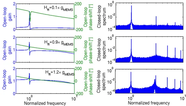
Figure 1.13: Simulations of the effect of the feed-through transmission in SOLs

(1.35) The corresponding frequency resolution is thus:

σfr = 1 ∂ψM EM S ∂f (fosc) Ô Tmeas◊ C Sthermo F2 l≠c + SM EM S_th¯ |Fl≠c◊ HmechaHdet|2 + Selec

|Fl≠c◊ HmechaHdetHconnec|2

D

(1.36) F_l≠c and Sthermo are intrinsically limited by the MEMS characteristics. It is

im-portant to design a MEMS with a strong detection gain, low MEMS-to-electronics connection losses and a low electronic noise in order to achieve a oscillator frequency resolution as close as possible to its ideal value defined as:

σfr≠ideal = fr 2QF_l≠c Û Sthermo Tmeas if Hf t π gM EM S. (1.37)

1.3.1.3 Effect of feed-through transmission in SOLs

Subsection 1.1.2 describes how ∂ψM EM S

∂f

-fr reduces with the feed-through

transmis-sion and thus the frequency resolution can be degraded. Moreover, it can be shown that the feed-through can create some parasitic oscillations that can further reduce the performance of the oscillator. Simulations were made for different levels of feed-through transmission gain on a similar loop than depicted in figure 1.11a. The

(34)

1.3 Closed loop resonant frequency tracking feed-through is modeled with a real gain independent of the frequency. The ampli-tude of the oscillations are controlled with a saturation block. The phase-shift of the loop is adjusted with a block having the following transfer function: 1≠jf/fc

1+jf /fc that

has a gain equal to 1. The results of the simulations are depicted in figure 1.13 and show that parasitic oscillations can appear in the loop. Indeed, the feed-through modifies the gain and phase-shift of the MEMS resonator and thus the oscillation conditions can also be satisfied at other frequencies.

Similarly to the design of electronic amplifiers, one can impose some margin on the gain of the loop at frequencies where the open-loop phase-shift crosses n ◊ 2π (n being an integer). For example, in the realizations described in chapter 3, a gain of 10 dB was imposed between the gain at fr and the gain at frequencies where the

open-loop phase-shift crosses n ◊ 2π.

1.3.1.4 Nonlinear self-oscillating loop

It should be mentioned that the design of a purely linear electronic circuit is impos-sible in practice due to the quadratic response of CMOS transistors. Imperfections created by nonlinear parts of the oscillators (that will be described in this subsec-tion) are therefore present for all SOL but with different degrees of degradations in the frequency resolution. Moreover, the design and the realization of a highly linear phase-shifter and an amplitude limiter can be difficult and expensive to fabricate. One can find examples whereby a saturation block is implemented rather than au-tomatic gain control to limit the oscillations amplitude [Gelb 1968, Arndt 2010, Akgul 2009, Verd 2008]. This is mainly because its implementation can be very simple. It uses an electronic amplification block that has a low dynamic range, i.e. the electronics saturates and its gain reduces when the input amplitude is larger than its dynamic range. The gain of the sustaining electronics reduces as the am-plitude of the oscillation in the system grows and thus the steady-state oscillation amplitude can be controlled. It is also possible for some MEMS topologies to use the nonlinearity of the MEMS resonator as a saturation mechanism. On the other hand, the distortions and the nonlinear behavior of the saturation block can modify the contribution of the noise sources on the resolution of the oscillator. The effect is complex and was rarely theoretically treated in the literature [Demir 2000]. How-ever, based on a Taylor expansion, a simple model of the nonlinear electronic circuit transfer function H_elec≠NL can be:

H_elec≠NL = Helec

1

1 + HD2velec+ HD3velec2 + ...

2

, (1.38)

where Helec is the linear electronic circuit transfer function, velec is the complex

amplitude of the electronics input signal, HD2 and HD3 are constant coefficients

that can be determined from the electronics nonlinear behavior. In the case of small nonlinearity, it is assumed that HD2velec π 1 and HD3velec2 π 1. One can introduce

an additive noise to the input signal:

(35)

Chapter 1 Harmonic detection of resonance where vnoise(t) respects S_v_elec = F [Γ_τ(vnoise(t))] and E {vnoise(t)} π v_elec (i.e. the

noise is small compared to the signal). The electronics output signal is (if only the 2nd _{harmonic distortion is considered: HD}

3 = 0)

vact(t) = Helec{veleccos (2πfosct) + vnoise(t) + (1.40)

HD2

Ë

v2

eleccos2(2πfosct) + v

2

noise(t) + 2veleccos (2πfosct) vnoise(t)

ÈÔ

. The term v2

eleccos2(2πfosct) introduces harmonics at 2 ◊ fosc and does not affect

the frequency resolution of the oscillator. The term v2

noise(t) can be considered as

negligible compared to the other term because E {vnoise(t)} π v_elec and HD₂v_elec π

1 implies that HD2E{v2noise(t)} π velec. The signal vnoise(t) can be expressed by its

one-side Fourier transform: vnoise(t) =

´Œ

0 Vnoise(ν) exp (≠j2πνt) dν. Thus:

vact(t) = Helec

I

veleccos (2πfosct) +

ˆ Œ

0 |V

noise(ν)| cos (2πνt + arg Vnoise(ν)) dν+

HD2

C

2veleccos (2πfosct)

ˆ Œ

0 |V

noise(ν)| cos (2πνt + arg Vnoise(ν)) dν

DJ . (1.41) Thus: vact(t) = Helec Ó

veleccos (2πfosct) + F≠1[Vnoise(ν)] +

velecHD2F≠1[Vnoise(fosc+ ν)] + velecHD2F≠1[Vnoise(fosc≠ ν)]

Ô

(1.42) The nonlinearity create some frequency aliasing and up-converts the flicker noise close to the oscillating frequency. The figure 1.14 illustrates the aliasing of the colored noise around the oscillation frequency. Note that this computed phase-noise corresponds to Sϕelec+M EM S that is the phase-noise injected in the loop. The Leeson’s

formula then describes how the injected phase-noise is shaped by the closed-loop. It is also possible to introduce in the sustaining electronics a comparator so that the output signal is in a two-state regime: the signal is either equal to a voltage V1 or

V2. With this architecture, the oscillation amplitude is controlled with ease through

V1 and V2. More importantly, since the comparator output signal is logic, digital

architectures can be used what simplifies the realization of the phase-shifter and any other filters. For example, the phase-shifter block can be realized using Delay-Lock-Loop (DLL). A DLL can introduce any desired phase-shift whatever the signal frequency is [Susplugas 2004]. Comparator can also be applied in order to filter other frequencies than fr, assuming that their amplitude are small compared to the

one at fr [Bahreyni 2007]. The drawback of this topology is that it introduces large

distortions, thus the issues inherent to the saturation blocks are emphasized.