HAL Id: hal-01397666
https://hal.archives-ouvertes.fr/hal-01397666v2
Submitted on 8 Jan 2018
HAL is a multi-disciplinary open access
archive for the deposit and dissemination of
sci-entific research documents, whether they are
pub-lished or not. The documents may come from
teaching and research institutions in France or
abroad, or from public or private research centers.
L’archive ouverte pluridisciplinaire HAL, est
destinée au dépôt et à la diffusion de documents
scientifiques de niveau recherche, publiés ou non,
émanant des établissements d’enseignement et de
recherche français ou étrangers, des laboratoires
publics ou privés.
Adaptive Feedforward and Feedback Control for Cloud
Services
Sophie Cerf, Mihaly Berekmeri, Bogdan Robu, Nicolas Marchand, Sara
Bouchenak, Ioan Doré Landau
To cite this version:
Sophie Cerf, Mihaly Berekmeri, Bogdan Robu, Nicolas Marchand, Sara Bouchenak, et al.. Adaptive
Feedforward and Feedback Control for Cloud Services. IFAC WC 2017 - 20th IFAC World Congress,
Jul 2017, Toulouse, France. pp.5504 - 5509, �10.1016/j.ifacol.2017.08.1090�. �hal-01397666v2�
Adaptive Feedforward and Feedback Control for
Cloud Services
Sophie Cerf∗Mihaly Berekmeri∗Bogdan Robu∗Nicolas Marchand∗
Sara Bouchenak∗∗Ioan D. Landau∗
∗Univ. Grenoble Alpes, CNRS, GIPSA-lab, F-38000 Grenoble, France {sophie.cerf,mihaly.berekmeri,bogdan.robu,nicolas.marchand,
ioan-dore.landau}@gipsa-lab.fr
∗∗Universit´e de Lyon, INSA-Lyon, CNRS, LIRIS, F-69621 Lyon, France [email protected]
Abstract:The use of cloud services is becoming increasingly common. As the cost of these services
is continuously decreasing, service performance is becoming a key differentiator between providers. Solutions that aim to guarantee Service Level Objectives (SLO) in term of performance by controlling cluster size are already used by cloud providers. However most of these control solutions are based on static if-then rules, they are therefore inefficient in handling the highly varying service dynamics of cloud environments. Client concurrency, network bottlenecks or non homogeneity of resources are just a few of the many causes that make the behavior of cloud services highly non linear and time varying. In this paper a novel control theoretical approach realizing resource allocation is presented that is robust to these phenomena. It consists of PI and feedforward controller adapted online. A stability analysis of the adaptive control configuration is provided. Simulations using a cloud service model taken from the literature illustrate the performance of the system under various conditions. The use of adaptation significantly improves control efficiency and robustness with respect to variations in the dynamic of the plant.
Keywords:control of computing systems, adaptive control, cloud computing, PI and feedforward control, MapReduce
1. INTRODUCTION
In the last decades, the world has faced a steep surge in the amount of produced data. This brings novel challenges for their storage and analysis. Many new programming paradigms have emerged to face the specificity of so called Big Data, such as MapReduce or Spark. Cloud computing, with its promise of barely unlimited storage and processing capabilities, is becom-ing an increasbecom-ingly attractive solution. One of the biggest ap-peals of cloud computing is the on-demand assigning of a large group of shared hardware resources to software applications, called elastic resource provisioning, but there is a growing need for frameworks that efficiently deal with the dynamics of cluster resources (Lorido-Botran et al., 2014).
Current autonomic resource provisioning approaches that are deployed in public clouds don’t work well for real time appli-cations. In most clouds, if an application has to meet run time criteria, it is up to the human application manager to decide the amount of resources it needs. When the manager is notified that the application is running slowly, it requires high level of expertise to decide on how much to intervene. The difficulty of the task is increased by the fact that the optimal configu-ration can vary due to the shared use of hardware resources or workloads fluctuations over time (Ari et al., 2003), among
1 This work has been partially supported by the LabEx PERSYVAL-Lab
(ANR-11-LABX-0025-01) funded by the French program Investissement d’Avenir.
2 This work has been supported, in part, by the European FP7 research project
AMADEOS Grant Agreement 610535 on Systems of Systems.
many other factors (Koh et al., 2007). Therefore, there is a need for fully automatized and robust cluster scaling algorithms able to deal with these disturbances. Ensuring service performance is essential as missing deadlines result in consequent financial losses. It is estimated that an on-line brokerage industry service unavailability costs around 100.000$ per minute. For on-line shopping companies, page load-time should not be more than 2 seconds or users tend to give up their shopping, resulting in revenue loss for companies (Nah, 2004). Cloud providers have to guarantee service performance and availability in order to win users’ loyalty.
Ensuring the performance of cloud services is a highly complex challenge. A cloud service behavior varies over time due to the dynamic of its environment (hardware, network, etc.). As cloud providers desire to maximize the utilization of their clusters, they have mechanisms for the dynamic reallocation of unused resources in the cluster, which further add to the variability of system performance. Hence, even with the same workload and the same resource amount, an application performance may vary depending on how noisy neighboring applications are. Moreover, cloud services are highly complex paradigms that run on top of multiple software stacks, making their behavior regarding to resource provisioning highly non linear.
Several solutions to deal with performance management of cloud services have recently emerged. Current approaches can be separated into four categories: static, reactive, predictive and combined approaches. In the industry, static deployments are the standard and usually tuned based on the application peak
de-mand and are generally over-provisioned. Reactive approaches are based on reacting to an input metric such as the current CPU utilization, the request rate or the service time by adding or removing servers as necessary (Hwang et al., 2016). Some public cloud providers such as the Amazon Auto Scaler offer the framework for reactive techniques but it is up to the user to define the scaling thresholds, which is very difficult, not reliable and requires great expertise. One of the most advanced reactive techniques are those which use queuing theory analytic models to decide capacity requirements based on the workload count (Gandhi et al., 2012). A different approach consists of us-ing predictive techniques to estimate the future load of a service and provision accordingly (Nguyen et al., 2013). There are also few solutions which try to mix the advantages of prediction and reaction into combined techniques, see Ali-Eldin et al. (2012). To our knowledge there is no work in the state of the art that aims at looking into this issue of resource provisioning from a robustness point of view, for instance through control adap-tation regarding system configuration and environment varia-tions. A solution able to be efficient no matter the workload, network or hardware state is missing.
In this article, a control theoretical approach is presented which aims at controlling cloud services performance using cluster scaling. On-line mechanisms that use information about past states of the systems to derive adequate system configura-tion are novel and promising approaches in computer science. Hellerstein et al. (2004) highlighted the promise of control the-ory, in providing a mathematical basis for the on-line adaptation of software systems, over a decade ago. Recently, the increasing number of publications in the field of control for computing systems shows the emergence of this new field for automatic control, see Patikirikorala et al. (2012) for a survey. The main asset of control theory is the mathematical guarantees it pro-vides that can be further utilized by cloud providers to erect
their Service Level Agreement (SLA).3
The control developed in this paper is composed of a reactive part (a feedback PI controller) that ensures steady state system convergence; and an predictive feedforward controller to ensure disturbance rejection. Our control is made robust with the ad-dition of an adaptation algorithm that estimate the feedforward gain. The second major contribution of this article is the use of real systems for our developments and tests. As requests processed by Big Data cloud services are highly diverse and data and/or computing intensive, studying those system with realistic scenarios is a real challenge. MRBS (a benchmark suite for the Big Data paradigm MapReduce) enables to run realistic workloads of multiple jobs and even to consider concurrency issues. The use of MRBS on a real cloud enables to truly capture the behavior of cloud services in their every-day IT companies usage.
The remaining of the paper is organized as follows: after an introduction to MapReduce (the use case used to illustrate the control approach) and an overview of its modeling, the adaptive control algorithm is presented. Stability analysis is performed and control validation is done through simulation. Finally, conclusion are drawn and future development avenues are given.
2. MAPREDUCE USE CASE
As an framework to develop and test our methodology, we chose a cluster running MapReduce jobs . This choice has been
3 SLA is as a part of a service contract, where services are formally defined.
motivated by the fact that MapReduce is one of the most pop-ular parallel processing paradigms for Big Data systems cur-rently in use. MapReduce was developed by Google in the last decade as a general parallel computing algorithm running on distributed platforms such as clouds that would automatically handle job and data management (data partitioning, consistency and replication, task distribution, scheduling, load balancing and fault tolerance (Dean and Ghemawat, 2008)). Nowadays, numerous IT leaders such as Yahoo, Facebook or LinkendIn use versions of MapReduce. MapReduce is a general paradigm that aims at being able to treat extremely diverse requests such as data mining or recommendation algorithms. Ensuring ac-ceptable performance of MapReduce jobs is essential for all users, and thus became a priority for clouds providers where MapReduce is deployed.
To understand why assuring performance in MapReduce clus-ters is such a challenge, a light analysis of how MapRe-duce works is presented here. MapReMapRe-duce is a programming paradigm developed for parallel, distributed computations over very large amounts of data. The initial implementation of MapReduce is based on a master-slave architecture, where the master node is in charge of task scheduling, monitoring and resource management and the slave nodes take care of start-ing and monitorstart-ing local mapper and reducer processes. For a user to run a MapReduce job, at least three things need to be supplied to the framework: the input data to be treated, a Map function, and a Reduce function. From the control point of view, the Map and Reduce functions can be only treated as black box models since they are entirely application-specific, and we do not have a priori knowledge of their behavior. Without some profiling, no assumptions can be made regarding their run time, resource usage or the amount of output data produced. On top of this, many factors (independent of MapReduce configuration parameters: input data, Map and Reduce functions) are identi-fied that influence job performance: CPU, input/output skews, software failures (Sangroya et al., 2012), servers homogene-ity assumption not holding up (Anjos et al., 2015), and bursty workloads (Ghit et al., 2014) among others. All the sources of disturbances specific to clouds (concurrency, network skews (Li et al., 2015), hardware failures, etc.) can be added to the variability of our system, especially when MapReduce is exe-cuted on a public cloud, as they are often more volatile. For a client using MapReduce, it is essential to have guarantees in term of service performance, dependability or costs. For instance, an e-commerce company running MapReduce to per-form sale recommendation based on client preferences needs to have the list of recommended products in a few tenth of seconds, otherwise their webpage will take too much time to be loaded. From the cloud provider point of view, this service time (the time it takes for a user request to be treated) is thus a performance metric that has to be monitored.
One simple action that can be done to control the on-line service time is to modify the number of resources of the cloud allocated to the jobs. For the MapReduce use case, adding resources, commonly known as nodes, to the cluster will increase the number of Map and Reduce functions processing the input data leading to a reduction of the service time. If the number of resources (nodes) diminishes, the results are converse. The cluster size is then our control signal.
However, in the case of public clouds, multiple clients send requests at the same time thus generating a varying input
workload which influences the service performance. If multiple concurrent jobs are running, the amount of resources allocated for each job is reduced and thus the job service time increases. As the workload of the system is independent of the cloud provider we will consider it as a disturbance. Mathematical formulation of the system modeling is given below in Section 3.
3. MAPREDUCE MODELING
In order to derive a model of MapReduce, Hadoop (its most used open source implementation) has been implemented on a real cluster and real-life requests are launched. The experiments used for the modeling process were run using the MapRe-duce Benchmark Suite (MRBS) developed by Sangroya et al. (2012). MRBS is a performance and dependability benchmark suite for MapReduce systems that can emulate several types of workloads and inject different fault types into a MapReduce system. The workloads emulated by MRBS are selected to represent a range of loads, from the compute-intensive to the data-intensive (e.g. business intelligence - BI) workload. One of the strong suits of MRBS is to emulate client interactions, which may consist of one or more MapReduce jobs run at the same time. A data intensive BI workload is selected for our experiments but other types of workloads can be used as well. It consists of a decision support system for a wholesale supplier. Each client interaction emulates a typical business oriented query run over a large amount of data (10GB here). All the nodes in the cluster were on the same switch to minimize network skews. The experiments were conducted on Grid5000, on a single cluster of 60 nodes. Grid5000 is a French nation-wide cluster infrastructure made up of a 5000 CPUs, developed to aid parallel computing research (Cappello et al., 2005). Each node from the cluster used for the test has a quad-core Intel CPU of 2.53GHz, an internal RAM memory of 15GB, 298GB disk space and infiniband network.
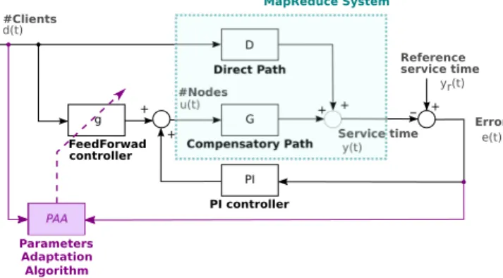
A dynamic model that predicts MapReduce cluster perfor-mance (i.e. the average service time of all submitted jobs) with respect to the number of nodes of the cluster and number clients sending requests was proposed and validated by experiments in Berekmeri et al. (2014) and is recalled in the blue dotted box of Fig. 1. yr(t) u(t) e(t) d(t) y(t) Service time #Nodes #Clients Reference service time G Compensatory Path D Direct Path + + - + PI PI controller g FeedForwad controller + + Error PAA Parameters Adaptation Algorithm MapReduce System
Fig. 1. MapReduce model and control schema
In Berekmeri et al. (2014), the system is considered linear in its operating region and the models were first identified as continuous transfer functions and then discretized using the
sampling period Ts= 30 sec. The resulting equation is4:
4 The complex variable z−1will be used to characterize the system’s behavior
in the frequency domain and the delay operator q−1will be used for the time domain analysis.
y(t) = D(q−1)d(t) + G(q−1)u(t) (1)
where y is the average service time of all jobs (the output),
u is the changes in the number of nodes in the cluster (the
control input) and d is the changes in clients (considered as a measurable disturbance). In the following we will use the error
e(t), which is the comparison of the measured service time with
its reference value, as a performance indicator of our control.
D(q−1) is the direct path transfer function, the link between the
disturbance and our performance metric, and G(q−1) represents
the compensatory path, it enables to modify the cluster size to control the service time. Both models were identified as first-order transfer function with delays, as described in eq. (2):
D(q−1) = bDq −1 1+ aDq−1q −rD G(q−1) = bGq −1 1+ aGq−1q −rG (2) with bD= 1.07, aD= −0.79, rD= 8, bG= −0.18, aG= −0.92 and rG= 5.
An analysis of the cloud system behavior detailed in Section 1 intuitively shows that the systems is non linear and time variant, thus the previous linear model is not accurate for a wide range of input or disturbance values. Therefore, for the remaining of the article an adaptive technique will be used and the system will be heavily tested by arbitrary varying the direct path time constant and static gain by a factor of two (from half to double the nominal value - see Section 4) in order to simulate real life conditions.
4. CONTROL FOR CLOUD SERVICES
The control presented in this paper consist of a PI controller introduced for asymptotic zero reference tracking error and a feedforward loop for dynamic disturbance compensation. A real time adaptation of the feedforward compensator is consid-ered in order to improve the performance since some parame-ters of the system are unknown and time-varing.
4.1 Adaptive FeedForward Control Law
Under the classical feedback-feedforward control loop in black of Fig. 1 (without the PAA adaptation path in purple) and using the eq. (2), the optimal value of the 0-order feedforward controller is given by:
u∗FF(t) = −bD(1 + aG)
bG(1 + aD).d(t) = g ∗d(t)
For the development of the adaptation algorithm, we will make the following hypotheses:
(H1) the effect of the PI controller can be neglected,
(H2) aD= aG,
(H3) rD= rGand are known.
Then the algorithm will be analyzed for the cases where hy-pothesis H1, H2 and H3 are violated.
Let us define the adaptive feedforward control algorithm as:
uFF(t) = ˆg(t)d(t) (3) where ˆgis given by ˆ g(t + 1) = ˆg(t) +αx(t + 1)e(t + 1) = ˆg(t) + αx(t + 1) 1+αx2(t + 1)e 0(t + 1) withα> 0 (4)
The filtered disturbance x is defined by:
x(t) = F(q−1)d(t) = q
−(rG+1)
where the a priori adaptation error e0(t + 1) is the value of the
regulation error at time t+ 1 and is based on the estimation of
ˆ
g(t): e0(t + 1) = e0(t + 1/ ˆg(t)). The a priori error e0(t + 1) is
considered as a performance metric for our system. One can
also define the a posteriori error e(t + 1) = e0(t + 1/ ˆg(t + 1))
which, based on eq (??), gives:
e(t + 1) = 1
1+αx2(t + 1)e
0(t + 1) (6)
Theorem For the scheme represented in Fig. 1, under the
hypothesis H1, H2 and H3, using the adaptive feedforward control given by eq. (3) to (5), one has:
limt→∞e(t + 1) = limt→∞e0(t + 1) = 0
for any initial conditions provided that:
H′(z−1) =1+ ˆaGz
−1
1+ aGz−1 (7)
is a strictly positive real transfer function.
RemarkThis later condition is always satisfied provided that
| ˆaG| < 1 (stability condition for the model) and ˆaG≤ 0.
ProofUnder the hypothesis H1, H2 and H3, the expression of
the error e for a fixed value ˆgis (see Fig. 1):
e(t + 1) = e0(t + 1) =bGq
−(rG+1)
1+ aGq−1(g
∗− ˆg)d(t + 1) (8)
Filtering d(t) by the filter F given in eq. (5) allows to rewrite eq. (8) as:
e(t + 1) = 1+ ˆaGq
−1
1+ aGq−1(g
∗− ˆg)x(t)
When replacing ˆgwith ˆg(t + 1) and neglecting the additional
vanishing term resulting from the non comutativity of time varying operators, one has:
e(t + 1) =1+ ˆaGq
−1
1+ aGq−1(g
∗− ˆg(t + 1))x(t) (9)
Eq. (9) has the standard form of an a posteriori adaptation
error equationand one can use straight-forwardly the results of Landau et al. (2011), Chapter 3, Theorem (3.2).
RemarkThe proof have shown the convergence of the
adapta-tion error (i.e. the performance variable). However, the
conver-gence of ˆg→ g∗is related to the richness of d.
4.2 Removing the hypotheses H1, H2 and H3
H1: the effect of the PI controller can not be neglected The continuous time PI controller has the transfer function:
PI(s) = KI
s + KP
Using the difference approximation 1− q
−1
TS
for differential operator one gets:
PI(q−1) =KITS+ KP− KPq −1 1− q−1 = r0+ r1q−1 1− q−1 = BK(q−1) AK(q−1) Using the results of Landau et al. (2016), Chapter 15, Section 15.17, eq. (15.86) for our particular scheme (with the values
AK = 1 − q−1, BK= r0+ r1q−1, BG= bGq−(rG+1), AG= 1 + aGq−1, S = 1, AM= 1, BM= 0), one gets: e(t + 1) = q −(rG+1)bG(1 − q−1)[g∗− ˆg(t + 1)]d(t) (1 + aGq−1)(1 − q−1) + bG(r0+ r1q−1)q−(rG+1) (10)
Using the parameter adaptation algorithm given in Section 4.1, the stability condition becomes that the following transfer function
H′′(z−1) = (1 − z
−1)(1 + ˆaGz−1)
(1 + aGz−1)(1 − z−1) + bG(r0+ r1z−1)z−(rG+1)
(11) should be a strictly positive real transfer function.
RemarkIf this condition is not satisfied, taking into account
eq. (10) one can use instead of the filter F given in eq. (5) the
filter FPI:
FPI(q−1) = q
−(rG+1)ˆbG(1 − q−1)
(1 + ˆaGq−1)(1 − q−1) + ˆbG(r0+ r1q−1)q−(rG+1)
(12)
H2: aD6= aG Denoting the unmeasurable output of the
dis-turbance propagation path D(q−1) by z(t), eq. (10) becomes in
the presence of the PI controller:
e(t + 1) = H′′(q−1) ([g − ˆg(t + 1)]d(t) + [aG− aD]z(t)) (13)
Since the adaptation does not affect directly the second term in the left hand side of eq. (13), we have to analyze its influence. As z(t) is the output of an asymptotically stable plant whose input is bounded, it will also be bounded. Therefore the signal
δ(t) = [aG− aD]z(t) will be bounded. Furthermore, due to the
PI controller, the effect of this disturbance term will go to 0 asymptotically in steady state for a constant value of d(t), since in eq. (10) the numerator of the transfer operator contains
(1 − q−1). This also holds if there is no PI since, for a constant
disturbance, the adaptation algorithm will interpret this term as an additional constant disturbance which will be canceled.
H3: rD 6= rG but known Hypothesis H3 on delays can be
relaxed to rG≤ rDboth known, but making the algorithm more
complex.
5. SIMULATION RESULTS
The validation of our adaptation mechanism will be done through comparison of the adaptive control algorithm with the optimal linear feedforward controller (computed on the
assumption that bG and aG are known) to the optimal linear
controller when the gain bG varies by 50%. We will then
analyze the introduction of a PI controller and finally study the robustness of our adaptive control algorithm performances
regarding the possible uncertainties on ˆaGin the filter used to
generate x(t).
Time (in min)
0 50 100 150 200 250 Disturbance (#clients) 6 8 10 12 14 16
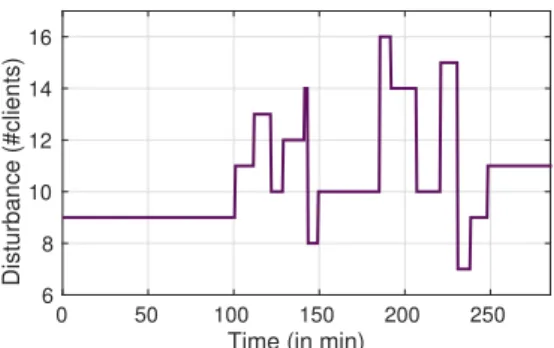
Fig. 2. Disturbance Scenario
The disturbance scenario we have simulated is represented in Fig. 2. After taking a constant value for stabilization of the system, the number of clients sending requests to our cloud service varies with inconstant frequency around the nominal
that H2 does not hold, that is to say that the two paths of our model do not have the same dynamics. H3 will always hold while from time to time a PI will be added, thus modifying assumptions of H1.
The behaviour of the optimal feedforward controller on the nominal model, on the compensatory model with a 50% differ-ent gain and evdiffer-entually coupled with a PI controller (parameters are issued from (Berekmeri et al., 2016)) are given in Fig. 3.
Time (in min)
0 50 100 150 200 250
Performance indicator (in sec)-40 -30 -20 -10 0 10 20 30 nominal model model 50% different
model 50% different with PI action
Fig. 3. Optimal Feedforward Controller performances for vari-ous scenarios
When simulating with the nominal model, the performance tends to 0 in steady state even if a transitory phase appears when a change in the disturbance occurs due to the difference of dynamics in direct and compensatory paths (H2 not holding). The modification of the real gain of the direct path changes the dynamics of the system and adds a steady state error (blue line). In order to deal with this, a PI is introduced that drives back our performance indicator to 0 in steady state. The PI is chosen with a really slow dynamics in order to prevent over reaction as explained in Berekmeri et al. (2016).
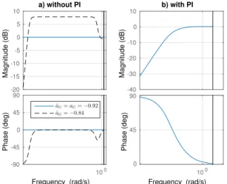
Magnitude (dB) -20 -15 -10 -5 0 5 10 100 Phase (deg) -90 -45 0 45 90 ˆ aG= aG=−0.92 ˆ aG=−0.84 a) without PI Frequency (rad/s) Magnitude (dB) -40 -30 -20 -10 0 10 100 Phase (deg) 0 45 90 b) with PI Frequency (rad/s)
Fig. 4. Bode diagram of the transfer functions given in eq.
(7) and (11) a) without PI for ˆaG= aG= −0.92 and for
ˆ
aG= −0.8 b) with PI for ˆaG= aG= −0.92
The stability of the adaptive control system without and with the PI controller is assured with the filter F given in eq. (5) since the transfer functions given in eq. (7) and (11) are strictly positive real as shown in the bode diagram of Fig. 4 (phase
between−90oand+90o).
Then the adaptive feedforward is simulated withα= 10−4and
ˆ
g(0) = 0 i.e. no a priori knowledge is considered. Once again
three scenarios are considered, the results are shown in Fig.
5: nominal model, 0.5bG and adding the PI controller to the
adaptive control algorithm.
Time (in min)
0 50 100 150 200 250
Performance indicator (in sec)
-20 -10 0 10 20 30 nominal model model 50% different
model 50% different with PI action
Fig. 5. Adaptive Feedforward Controller performances for var-ious scenarios
When simulating with the nominal model, the adaptive feed-forward control drives the performance indicator to 0 but with a longer convergence time than in the optimal simulation and with more oscillations. However, the adaptive control maintains the steady state to 0 even for the case with modified value of
bG. The addition of a PI controller considerably reduces the
convergence time and the magnitude of the transients.
The introduction of adaptation in the PI scenario enables the significant reduction of transient magnitudes and convergence times as can be seen in Fig. 6. Indeed, the error variance is reduced from 5.17 to 0.76 during the disturbance rejection phase (on the time horizon from 100 min to 300 min).
Time (in min)
0 50 100 150 200 250
Performance indicator (in sec)
-15 -10 -5 0 5 10 optimal feedforward adaptive feedforward
Fig. 6. Optimal and Adaptive Feedforward and PI Controller performances comparison, model 50 % different
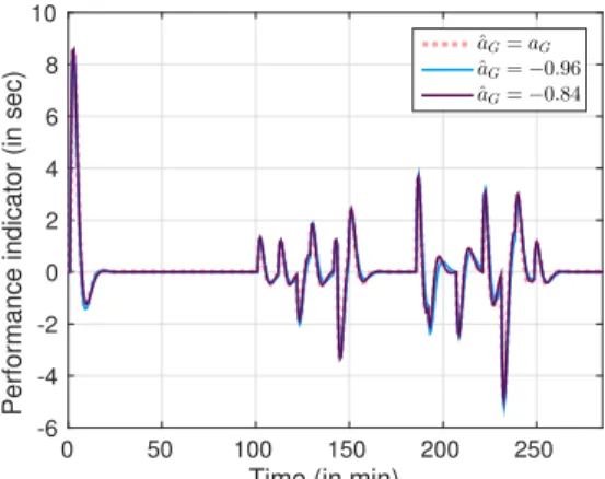
Fig. 7 illustrates the robustness of adaptation algorithm
perfor-mance combined with a PI with respect to the value of ˆaG in
the filter F. The compensatory model is considered with a 50% variation of its gain and the filter coefficient is taken with its
nominal value ( ˆaG= −0.92), with higher value ( ˆaG= −0.84)
and a lower value ( ˆaG= −0.96). These values reflect a
modifi-cation of the estimated time constant by a factor 2.
Neither the magnitude of the transients nor the convergence time change significantly when the filter pole varies. This al-lows to conclude that the performance of the adaptive controller is robust with respect to changes in the model dynamics (aG) or with respect to uncertainties in its estimation.
Time (in min)
0 50 100 150 200 250
Performance indicator (in sec)
-6 -4 -2 0 2 4 6 8 10 ˆ aG= aG ˆ aG=−0.96 ˆ aG=−0.84
Fig. 7. Robustness analysis of Adaptive Feedforward and PI Controller performance with respect to filter variations
6. CONCLUSION
This paper presents an adaptive control strategy that ensures efficient control for the performance of Cloud Services in term of service time, by dynamically controlling its resource cluster size. The control algorithm is based on a PI and an adaptive estimation of the feedforward gain. Simulations are based on a model of MapReduce, a well known Big Data cloud service, running realistic workloads on a real cloud. Results show that the adaptive control enables the reduction by at least a factor of 6 the variance of the service time compared to a PI and optimal feedforward when concurrent clients requests disturb the system. Moreover, the presented adaptive control has proven its robustness as it successfully manages to control the cloud service even when the physical system is significantly different from the considered model. The obtained results show the potential of the adaptive feedfoward control combined with a feedback controller.
This novel usage of adaptive control theory shows encouraging results. We believe that the use of control theory for cloud systems can be extended quite straightforwardly to other com-puting systems such as networks management or VM control as many similarities connect those different computing applica-tions.
Future works will consist in extending the proposed adaptation algorithm to improve its convergence behavior, as well as including more system specific constraints, such as delays or control signal quantification. Experiments to validate the adaptive control on a real cloud system, such as Amazon Web Service or Microsoft Azure, running realistic jobs are planned. Other service metrics such as availability, dependability or costs which are crucial for service providers and users will also be considered.
REFERENCES
Ali-Eldin, A., Tordsson, J., and Elmroth, E. (2012). An adaptive hybrid elasticity controller for cloud infrastructures. In IEEE
Network Operations and Management Symposium, 204–212. Anjos, J.C., Carrera, I., Kolberg, W., Tibola, A.L., Arantes, L.B., and Geyer, C.R. (2015). MRA++: Scheduling and data placement on mapreduce for heterogeneous environments.
Future Generation Computer Systems, 42, 22–35.
Ari, I., Hong, B., Miller, E.L., Brandt, S.A., and Long, D.D. (2003). Managing flash crowds on the internet. In 11th
IEEE/ACM Int. Symposium on Modeling, Analysis and Sim-ulation of Computer Telecommunications Systems, 246–249.
Berekmeri, M., Serrano, D., Bouchenak, S., Marchand, N., and Robu, B. (2014). A Control Approach for Performance of Big Data Systems. In 19th IFAC World Congress, volume 19. Berekmeri, M., Serrano, D., Bouchenak, S., Marchand, N., and Robu, B. (2016). Feedback Autonomic Provisioning for Guaranteeing Performance in MapReduce Systems. to
appear in IEEE Transactions on Cloud Computing.
Cappello, F., Caron, E., Dayde, M., Desprez, F., Jegou, Y., Primet, P., Jeannot, E., Lanteri, S., Leduc, J., Melab, N., Mornet, G., Namyst, R., Quetier, B., and Richard, O. (2005). Grid’5000: A large scale and highly reconfigurable grid experimental testbed. In Proceedings of the 6th IEEE/ACM
Int. Workshop on Grid Computing, 99–106.
Dean, J. and Ghemawat, S. (2008). Mapreduce: simplified data processing on large clusters. Communications of the ACM, 51(1), 107–113.
Gandhi, A., Harchol-Balter, M., Raghunathan, R., and Kozuch, M.A. (2012). Autoscale: Dynamic, robust capacity man-agement for multi-tier data centers. ACM Transactions on
Computer Systems (TOCS), 30(4), 14.
Ghit, B., Yigitbasi, N., Iosup, A., and Epema, D. (2014). Bal-anced resource allocations across multiple dynamic MapRe-duce clusters. ACM SIGMETRICS Performance Evaluation
Review, 42(1), 329–341.
Hellerstein, J.L., Diao, Y., Parekh, S., and Tilbury, D.M. (2004).
Feedback control of computing systems. John Wiley & Sons. Hwang, K., Bai, X., Shi, Y., Li, M., Chen, W.G., and Wu, Y. (2016). Cloud performance modeling with benchmark evaluation of elastic scaling strategies. IEEE Transactions
on Parallel and Distributed Systems, 27(1), 130–143. Koh, Y., Knauerhase, R., Brett, P., Bowman, M., Wen, Z., and
Pu, C. (2007). An analysis of performance interference
effects in virtual environments. In IEEE Int. Symposium on
Performance Analysis of Systems & Software, 200–209. Landau, I.D., Airimioaie, T.B., Castellanos-Silva, A., and
Con-stantinescu, A. (2016). Adaptive and Robust Active Vibration
Control: Methodology and Tests. Springer.
Landau, I.D., Lozano, R., M’Saad, M., and Karimi, A. (2011).
Adaptive control: algorithms, analysis and applications. Springer Science & Business Media.
Li, Z., Shen, Y., Yao, B., and Guo, M. (2015). OFScheduler: A dynamic network optimizer for MapReduce in heteroge-neous cluster. Int. Journal of Parallel Programming, 43(3), 472–488.
Lorido-Botran, T., Miguel-Alonso, J., and Lozano, J.A. (2014). A review of auto-scaling techniques for elastic applications in cloud environments. Journal of Grid Computing, 12(4), 559–592.
Nah, F.F.H. (2004). A study on tolerable waiting time: how long are web users willing to wait? Behaviour & Information
Technology, 23(3), 153–163.
Nguyen, H., Shen, Z., Gu, X., Subbiah, S., and Wilkes, J. (2013). Agile: Elastic distributed resource scaling for infras-tructure - as - a - service. In Proceedings of the 10th Int.
Conference on Autonomic Computing (ICAC), 69–82. Patikirikorala, T., Colman, A., Han, J., and Wang, L. (2012).
A systematic survey on the design of self-adaptive software systems using control engineering approaches. In
Proceed-ings of the 7th IEEE Int. Symposium on Software Engineer-ing for Adaptive and Self-ManagEngineer-ing Systems, 33–42. Sangroya, A., Serrano, D., and Bouchenak, S. (2012). MRBS:
towards dependability benchmarking for Hadoop Mapre-duce. In EuroPar’12: Parallel Processing Workshop, 3–12.