A Test Bench for Distortion-Energy Optimization of a DSP-Based H.264/SVC Decoder

HAL Id: hal-00560030

https://hal.archives-ouvertes.fr/hal-00560030

Submitted on 27 Jan 2011

HAL is a multi-disciplinary open access

archive for the deposit and dissemination of

sci-entific research documents, whether they are

pub-lished or not. The documents may come from

teaching and research institutions in France or

abroad, or from public or private research centers.

L’archive ouverte pluridisciplinaire HAL, est

destinée au dépôt et à la diffusion de documents

scientifiques de niveau recherche, publiés ou non,

émanant des établissements d’enseignement et de

recherche français ou étrangers, des laboratoires

publics ou privés.

A Test Bench for Distortion-Energy Optimization of a

DSP-Based H.264/SVC Decoder

Fernando Pescador, Eduardo Juarez, David Samper, César Sanz, Mickaël

Raulet

To cite this version:

Fernando Pescador, Eduardo Juarez, David Samper, César Sanz, Mickaël Raulet. A Test Bench

for Distortion-Energy Optimization of a DSP-Based H.264/SVC Decoder. Digital System Design:

Architectures, Methods and Tools (DSD), 2010 13th Euromicro Conference on, 2010, France. pp.123

-129, �10.1109/DSD.2010.109�. �hal-00560030�

A Test Bench for Distortion-Energy Optimization of a

DSP-Based H.264/SVC Decoder

F. Pescador, E Juarez, D. Samper and C. Sanz

Grupo de Diseño Electrónico y Microelectrónico (GDEM) Madrid, Spain

{pescador, ejuarez, dsamper, cesar}@sec.upm.es

M. Raulet

Rennes, France mraulet@insa-rennes.fr

Abstract— This paper describes an OMAP-based real-time test bench to find the Pareto frontier of an H.264/SVC decoder within a distortion-energy optimization space. A metric to estimate video distortion is introduced. In addition, energy consumption estimates are obtained from real-time measurements of the computational load. Finally, test bench operation is successfully demonstrated with different H.264/SVC-compliant sets of sequences.

Keywords: Distortion-Energy optimization, Scalable Video Coding, Video Quality Estimation.

I. INTRODUCTION

System-level energy optimization of battery-powered multimedia embedded systems has recently become a design goal. The poor operational time of multimedia terminals makes computationally demanding applications impractical in real scenarios. For instance, the so-called smart-phones are currently unable to remain in operation longer than several hours [1]. Moreover, because no step change in energy densities of lithium-based batteries is predicted in the near future [2], storage technology improvements alone will achieve no significant increase in terminal operational time. System-level solutions to maximize operational time have already been proposed in the literature [3, 4, 5, 6]. However, despite the fact that degradations of perceived multimedia quality prevent technology user adoption [7], this performance parameter has usually been discarded as an optimization goal.

A multi-objective optimization that simultaneously considers perceived video quality and global energy consumption has already been envisaged [8]. The aim is to vary the perceived multimedia quality to achieve the maximum operational time. Generally speaking, both quality and system energy consumption depend on parameters such as power amplifier transmission power, linearity and video distortion, among others [10]. The set of possible values of these control parameters can be viewed as a set of points in a multidimensional control space. Depending on the battery state-of-charge, efficient multimedia terminals can search the set of system control points that simultaneously optimize operational time and multimedia quality [10].

A Pareto-optimum system control point [11] is found when an increase in the terminal operational time is only

accomplished at the expense of multimedia quality or, conversely, when further improvement in quality is only realized with a simultaneous decrease in operational time. The set of Pareto-optimum system control points is known as the Pareto frontier [12].

To avoid the excessive overhead of finding the optimum system control points at runtime, the Pareto frontier can first be characterized at design time based on a scenario definition; later, at runtime, this can be used to select an optimum system control point as a function of the battery state-of-charge [8]. It is worth noting that achieving the maximum quality is equivalent to reaching the minimum distortion; similarly, accomplishing the maximum operational time is equivalent to reaching the minimum global energy consumption.

The methodology to obtain the Pareto frontier at design time could be summarized as follows. A scenario in which a multimedia terminal receives and decodes a Transport Stream (TS) is assumed. In this context, network- and multimedia-related features, especially real-time video decoding, will be the main greedy energy consumers. For instance, Neuvo [13] indicates that two-thirds of the 3W power budget of a third-generation (3G) mobile phone in a 384 Kbps video streaming scenario accounts for network- and multimedia-related features. Next, the quality and consumption behavior of the multimedia terminal are estimated or measured for a defined scenario based on the system control points. Finally, Pareto-optimum system control points belonging to the Pareto frontier are identified to be used at runtime.

Although multi-objective terminal characterizations have already been proposed in the literature [10], to the best of our knowledge, no detailed results have been presented on terminals with current state-of-the-art video decoder implementations. This paper describes an OMAP-based [14] real-time test bench to estimate the Pareto frontier of a video decoder embedded in a multimedia terminal within the distortion-energy optimization space.

The rest of the paper is organized as follows. In section II, a controllable energy consumption video decoder is described. Section III details the test bench used to characterize the Pareto frontier of a multimedia terminal. In section IV, the usage of the test bench is exemplified, and the results are shown. Finally, in section V, conclusions are drawn, and future work is proposed.

This work was supported by the Spanish Ministry of Science and Technology under grants TEC2009-14672-C02-01 and TEC2006-13599-C02-01.

II. SOLUTION BASED ON SCALABLE VIDEO CODING To control the energy consumption of a video decoder embedded in a battery-powered portable device, the H.264/SVC (Scalable Video Coding) standard [15], [16] is an appropriate choice. In this standard, the video compression is performed by generating a unique hierarchical bit-stream structured in several levels or layers of information, consisting of a base layer and several enhancement layers. The base layer provides basic quality. The enhancement layers provide improved quality at increased computational cost and energy consumption. Because the energy consumption depends on the particular layer to decode, an H.264/SVC decoder is a very well-suited solution for managing the energy consumption by selecting the appropriate layer. H.264/SVC was standardized as an annex of H.264/AVC standard in 2007 to cover the needs of scalability. It specifies three types of scalabilities: spatial, temporal and quality.

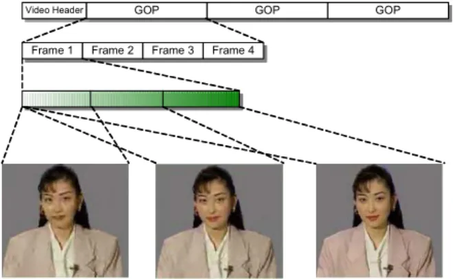
In a temporally scalable video sequence, several frame rates (temporal layers) of a video sequence can be chosen when decoding. Fig. 1 shows an example of a Group of Pictures (GOP) where the user can select three plausible frame rates. If the device decodes the four frames of the GOP (I1, B1, B2, B3), a full-frame-rate sequence will be obtained. If the decoder discards B1 and B3 frames and only decodes I1 and B2, a half-frame-rate sequence will be achieved. The third case is a quarter-frame-rate sequence, which will be obtained when the decoder discards B1, B2 and B3 frames and only decodes I1.

I1 B1 B2 B3 I2

Fig. 1. Example of a GOP in a temporally scalable bit-stream. In a spatially scalable video sequence, several spatial resolutions (spatial layers) of the video frames can be chosen when decoding. Fig. 2 depicts an example of a spatial scalable bit-stream containing three possible resolutions. As can be seen, the information relating to the three resolutions of a frame is contained in the field reserved for such frame in the bit-stream.

Video Header GOP GOP GOP Frame 1

Res 1 Res 2 Res 3 Frame 2 Frame 3 Frame 4

Fig. 2. Example of a spatially scalable bit-stream.

In a quality-scalable video sequence (or SNR sequence), it is possible to select several quality levels (quality layers) when decoding. Fig. 3 shows an example of a quality scalable bit-stream with three types of quality. The information relating to the three qualities of a frame is contained in the space reserved for this frame in the bit-stream.

Video Header GOP GOP GOP Frame 1 Frame 2 Frame 3 Frame 4

Fig. 3. Example of a quality-scalable (SNR) bit-stream.

Finally, the three types of scalability specified in H.264/SVC can be combined into a bit-stream. As an example, consider a coded video sequence that has three temporal layers, three spatial layers and three quality layers. An H.264/SVC decoder that has a medium charged battery may decode, for instance, the third spatial layer to get full spatial resolution, the second temporal layer to get half temporal resolution and the first quality layer to get a low-quality level. A decoder that has a fully charged battery might decode the entire bit-stream to get the full temporal and spatial resolution as well as the higher quality.

III. TEST BENCH A. Test bench Description

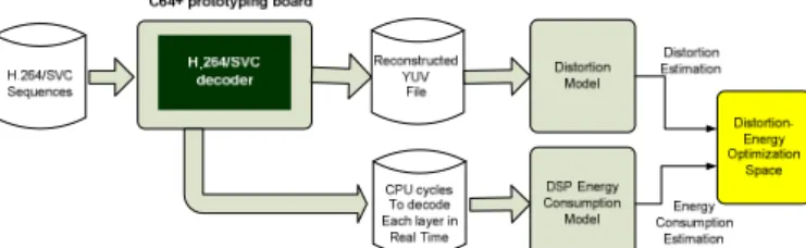
To find the Pareto-optimum system control points that minimize the distortion of the decoded sequence and the decoder energy consumption, the test bench shown in Fig. 4 has been implemented.

The test bench consists of a decoder that implements the standard H.264/SVC using a development platform based on a C64+ [17] DSP core from Texas Instruments. The test bench decodes the layers of a sequence and measures the number of CPU clock cycles required to decode each frame.

Using an energy consumption model of the DSP and measuring the processor computational load, it is possible to estimate the energy consumption of the decoder for each layer.

On the other hand, the distortion of the decoded sequences is estimated by assigning to each of the layers a value as a function of the quality, spatial and temporal resolutions.

Both estimations define a two-dimensional optimization space in which it is possible to select the combinations that simultaneously maximize both parameters.

Fig. 4. Test bench implemented to find the Distortion-Energy optimization points.

The following subsections describe the implementation of a H.264/SVC decoder, the selected DSP core, the generated sequences for the tests and the estimation models of energy consumption and distortion.

B. OpenSVC Decoder

IETR has developed the OpenSVC decoder [18], a C language baseline profile SVC decoder supporting all tools to deal with spatial, temporal and quality scalabilities. It is based on a fully compliant H.264 baseline decoder with most of the tools of the main profile. Only the interlaced coding and the weighted prediction are not supported because of their complexity for embedded systems. The performance of the OpenSVC decoder is up to 52 times faster than that of the JVSM decoder [19], which makes this decoder a good starting point in the development of a DSP-based SVC decoder.

The OpenSVC decoder has been developed to be compiled in a PC environment; thus, the code has been ported to the DSP development environment. In this porting process, the configuration of the real-time operating system has been defined, and the maximum size of the decoded frames has been reduced due to the memory limitations in the development platform.

To confirm the DSP-based decoder conformance, an automatic test has been developed to compare pixel by pixel the sequences decoded by the OpenSVC decoder running in a PC with the sequences generated by the DSP. The results of this comparison demonstrate that the sequences decoded by the PC version are identical to the sequences decoded by the DSP.

C. Prototyping Platform

The OMAP family of processors includes a DSP core based on the C64+. This core is the same as the one integrated in the TMS320DM6437 DSP [20]. A commercial development platform is available for this DSP. The conclusions related to energy consumption obtained for this DSP are directly applicable to the OMAP processors.

A simplified block diagram of the C64+ is shown in Fig. 5. A fixed-point core with two levels of internal memory (L1 and L2) and an internal DMA (IDMA) is used. The L1P memory/cache consists of a 32 KB memory space and the L1D memory consists of an 80 KB memory space. Both memories can be configured as cache memories, general-purpose memories or a combination of both. Finally, the L2

memory/cache consists of a 128 KB memory space, shared between the program and data. L2 memory can be configured as a general-purpose mapped memory, a cache memory, or a combination of both.

In the test bench, the L1P and L1D internal memories have been configured as 32 KB level-1 cache memories, and the L2 internal memory, as a 128 KB of level-2 cache memory.

The DSP includes other peripherals that will be interesting in near future for developing a complete multimedia terminal device as an Ethernet MAC (EMAC), an EDMA controller (EDMA3) and a video processing subsystem for video display.

Fig. 5. Architecture of the kernel C64+.

A commercial prototyping board [21] (Fig. 6) based on the DSP has been used to test the OpenSVC decoder and measure its performance as the number of CPU cycles spent to decode each frame of a specific layer. The board has a DSP working at 600 MHz, 128 MB of SDRAM external memory, 80 MB of Flash external memory and several interfaces.

The decoder performance has been measured in real time using a DSP internal timer. The timer is captured both at the beginning and at the end of a Network Abstraction Layer (NAL) decoding process. The difference between the two data is the time spent by the decoder for this NAL unit.

Fig. 6. The DSP-based development board.

The decoder has been migrated to the prototyping board, and a specific test application has been developed to measure the decoder performance. In this application, a test stream is read from a file and written into a stream buffer allocated in external memory. Subsequently, the DSP reads the stream from this memory, decodes it on a picture basis and writes the decoded picture into a buffer. The picture is also written into a file. Moreover, a file with real-time performance measurements is generated that includes the number of CPU cycles spent to decode each picture.

To execute automatic tests, a Perl script [22] has been generated using the script language available in Code Composer Studio [23]. This automatic test decodes all of the sequences and extracts profiling results in Excel file format. D. Distortion Model

Generally speaking, each type of scalability affects the distortion of decoded scalable streams differently. Spatial scalability influences the size of decoded frames; temporal scalability has an impact on video motion feeling, and quality scalability concerns Signal-to-Noise Ratio (SNR).

To have an objective measure of the global distortion of a decoded layer, L, the definition of a distortion parameter that includes the three kinds of scalabilities is needed. With this idea in mind, a normalized layer distortion parameter, δ(L), has been defined as the complement of the distance between the layer, L, and the maximum-distortion layer, LB.

) L , L ( d 1 ) L ( − _B δ = (1)

To measure the layer separation, the weighted L1

(Manhattan) distance has been selected:

i i 3 1 i i 1(X,Y) w x y WL ) Y , X ( d = =

∑

where the xi and yi are the scalability values of layers X and

Y, and wi are the weights for the spatial, temporal and quality

dimensions. Frame size (Fs), frame-rate (Fr) and bit-rate (Br) have been used as metrics of the spatial, temporal and quality scalabilities, respectively. Note that the metric used for quality scalability is the sequence bit-rate instead of the Peak-SNR (PSNR). Bit-rate and PSNR parameters are directly related and usually the decoders can be configured to obtain a specific bit-rate but not a PSNR.

Given the previous definition, the normalized layer distortion parameter can be calculated as indicated in equation (3) )} L ( QS ) L ( TS ) L ( DS { 1 ) L ( = − + + δ (3)

where DS(L), TS(L), and QS(L) are the spatial, temporal and quality scalability components of the interlayer distance, defined in equations (4-6). min min max 1 _{Fs(L) Fs} Fs Fs C ) L ( DS − − = (4) min min max 2 _{Fr(L) Fr} Fr Fr C ) L ( TS − − = (5) min min max 3 _{Br(L) Br} Br Br C ) L ( QS − − = (6)

o Ci are the scale coefficients,

∑

o L is the selected layer.

o Fs

( )

( )

( )

o Fs_max and Fs_min are the greatest and smallest layer frame sizes, respectively.

o Fr_max and Fr_min are the greatest and smallest layer frame-rates, respectively.

o Br_max and Br_min are the greatest and smallest layer bit-rates, respectively.

The scale coefficients, Ci, adjust the weight of each distance

scalability component, DS, TS, and QS. Their value varies between zero and one. Depending on the components to be highlighted, i.e. the distortion model to be considered, the scale coefficients are modified accordingly. For instance, in case the spatial component, DS(L), is the most significant one, the values of the scale coefficients could be C1 = 0.6, C2 = 0.2

and C3 = 0.2. As a consequence, the defined normalized layer

distortion parameter, δ(L), is a useful tool to study how a particular distortion model impacts on the device energy consumption.

E. Test Sequences

In order to assess the test bench depicted in Fig. 4, the well-known video sequence foreman (50 frames, YUV 4:2:0) has been encoded using a commercial H.264/SVC codec [24]. Three 9-layer sequences have been generated. The layer structure of each sequence consists of all the possible combinations among three spatial resolutions (CIF, QCIF, and subQCIF) and three frame-rates (24 fps, 12 fps, and 6 fps). In addition, each sequence has been encoded with different bit-rate (0.5 Mbps, 1.0 Mbps, and 2.0 Mbps).

As far as the codec parameters to generate the three test sequences concern, the GOP size equals 16 progressive frames, the Context-based Adaptive Binary Arithmetic Coding (CABAC) tool is used for entropy coding, the deblocking filter is active, all possible macroblock partitions are enable for intra- and inter-prediction, a maximum of three reference frames is allowed, and, at last, 3 B-frames are coded for each I- or P-frame.

For each test sequence layer, the values of the metrics defined in the previous section have been ordered and mapped into three indexes: D, T and Q. The D index designates the spatial resolution, the T index symbolizes the frame rate and the Q index denotes the bit-rate level. Each combination of D, T and Q values, i.e., a layer, defines a control point.

Since the quality, space and temporal scalabilities of the test sequences includes three possible values, the triplet (D, T, Q) defines a three-dimensional global control space with 27 control points (See Fig. 7). For instance, the control point associated in Fig. 7 with the base layer of the first encoded

sequence is (0, 0, 0), i.e. (subQCIF, 6 fps, 0.5 Mbps), and the maximum quality layer control point of the third encoded sequence is (2, 2, 2), i.e. (CIF, 24 fps, 2.0 Mbps).

Temporal (T) Quality (Q)

Spatial (D)

(2,2,2)

(0,0,0)

Fig. 7. Test sequences (D, T, Q)-triplet control space

Each test sequence includes three spatial resolutions (D = 0, 1 and 2) and three frame rates (T = 0, 1 and 2). As can be seen in Fig. 8, the 9 control points of a test sequence define a subset of the global control space. In particular, Fig. 8 shows the subset of the third sequence for Q = 2, i.e. 2 Mbps of bit-rate. The layers within the sequence are labeled from L0 to L8.

Note that three independent test sequences have been encoded instead of only one because neither the encoder nor the OpenSVC decoder supports bit-streams with 27 layers.

Temporal (T) Quality (Q) Spatial (D) S3-L0 S3-L1 S3-L2 S3-L3 S3-L4 S3-L5 S3-L6 S3-L7 S3-L8

Fig. 8. Control point set of the 2.0 Mbps test sequence (Q = 2). F. Energy Consumption Model

The device energy consumption model described by the manufacturer in [25] has been used. It is based on experimental measurements of devices that have been selected at the maximum end of energy consumption for production units. The manufacturer guarantees that no production units have average power consumption that exceeds the predicted values. This model is divided into two primary parts: baseline energy and activity energy.

Baseline energy describes energy consumption that is independent of any chip activity. This includes static power (leakage) and oscillator power. Baseline power depends on device operating frequency, voltage and temperature.

Activity energy describes the energy consumed by DSP active modules, i.e. CPU, external memory interfaces, peripherals, etc. Therefore, this consumption varies widely depending on the usage of on-chip resources. Activity energy depends on voltage and activity levels. The contribution of the major modules of the device to the activity energy can be measured independently. For each module, the model specifies a linear relation between the activity energy and the activity level. In turn, the module activity level depends on several parameters such as frequency, status, utilization, read/write balance, bus size and switching probability.

The energy consumption estimates of the DSP-based OpenSVC decoder have been obtained with the frequency value set at 600 MHz, the input voltage value at 1.2 V and the temperature value at 25ºC. With these settings, the corresponding baseline energy is 1.3 J for all of the test sequences. To estimate the activity energy of the model, only the CPU module has been considered.

IV. RESULTS

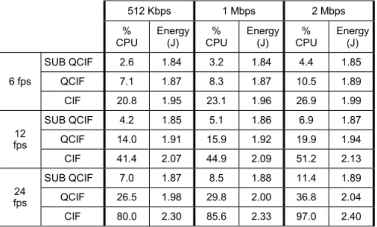
Using the test sequences defined in section III.E and the implemented test bench described in section Error! Reference source not found., the computational load needed to decode each layer of the example sequences has been measured. Applying the energy consumption model described in section III.F, an estimate of the active energy consumed to decode the layers of the test sequences has been obtained. Table I summarizes the computational load and the consumed active energy for each layer of foreman (0.5 Mbps, 1.0 Mbps, 2.0 Mbps). As can be seen from Table I, frame rate and frame size modifications are the main reason for active energy change (up to a 25%). In contrast, no significant increase (less than 5%) in active energy consumption is achieved varying the bit-rate from 0.5 Mbps to 2.0 Mbps.

TABLE I

CPU COMPUTATIONAL LOAD AND ESTIMATED ACTIVE ENERGY CONSUMPTION. 512 Kbps 1 Mbps 2 Mbps %

CPU Energy (J) CPU % Energy (J) CPU % Energy (J) 6 fps SUB QCIF 2.6 1.84 3.2 1.84 4.4 1.85 QCIF 7.1 1.87 8.3 1.87 10.5 1.89 CIF 20.8 1.95 23.1 1.96 26.9 1.99 12 fps SUB QCIF 4.2 1.85 5.1 1.86 6.9 1.87 QCIF 14.0 1.91 15.9 1.92 19.9 1.94 CIF 41.4 2.07 44.9 2.09 51.2 2.13 24 fps SUB QCIF 7.0 1.87 8.5 1.88 11.4 1.89 QCIF 26.5 1.98 29.8 2.00 36.8 2.04 CIF 80.0 2.30 85.6 2.33 97.0 2.40

Table II provides the values of the normalized layer distortion parameter, δ, for three distortion example models. The features of the defined models are the following:

o In Model 1, all scalability components (DS(L), TS(L), QS(L)) are of equal significance. The values of the scale coefficients are C1 = 0.333, C2 = 0.333 and C3 =

0.333. The distortion parameter of Model 1 is designated as δ1.

o In Model 2, DS(L), the spatial scalability component, is the most significant one. The values of the scale factors are C1 = 0.5, C2 = 0.25 and C3 = 0.25. The distortion

parameter of Model 2 is named δ2.

o In Model 3, the most significant scalability component is TS(L). The values of the scale factors are C1 = 0.25,

C2 = 0.5 and C3 = 0.25. The distortion parameter of

Model 3 is designated as δ3.

As shown in Table II, the normalized layer distortion parameter, δ, is a relative measurement. Effectively, in any of the distortion models, δ, varies from the minimum distortion (δ=0) for the (CIF, 24 fps, 2.0 Mbps) layer to the maximum distortion (δ=1) for the (subQCIF, 6 fps, 0.5 Mbps) layer. In any case, the distortion value distribution depends on the selected model.

TABLE II

DISTORTION PARAMETER (δ) FOR DIFFERENT DISTORTION MODELS.

δ1 δ2 δ3 24 fps fps 12 fps 6 fps 24 fps 12 fps 6 fps 24 fps 12 fps 6 512 Kbps SUB QCIF 0.67 0.89 1.00 0.75 0.92 1.00 0.50 0.83 1.00 QCIF 0.60 0.82 0.93 0.70 0.87 0.95 0.45 0.78 0.95 CIF 0.33 0.56 0.67 0.50 0.67 0.75 0.25 0.58 0.75 1 Mbps SUB QCIF 0.56 0.78 0.89 0.58 0.75 0.83 0.42 0.75 0.92 QCIF 0.45 0.71 0.82 0.53 0.70 0.78 0.37 0.70 0.87 CIF 0.22 0.44 0.56 0.33 0.50 0.58 0.17 0.50 0.67 2 Mbps SUB QCIF 0.33 0.56 0.67 0.25 0.42 0.50 0.25 0.58 0.75 QCIF 0.27 0.49 0.60 0.20 0.37 0.45 0.20 0.53 0.70 CIF 0.00 0.22 0.33 0.00 0.17 0.25 0.00 0.33 0.50

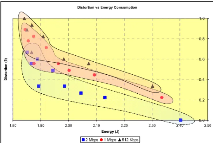
Fig. 9, Fig. 10 and Fig. 11 presents the Distortion-Energy optimization space for distortion model 1, model 2 and model 3, respectively.

The control points marked with a ▲ present the couple of distortion-energy values associated to the layers of sequence S1 (512 Kbps); the mark, ●, shows the control points associated with the layers of sequence S2 (1.0 Mbps) and, finally, the control points associated to the layers of sequence S3 (2.0 Mbps) are presented with a ■. In each figure, the control points belonging to the same test sequence are wrapped with a dashed line. As shown in the previous figures, the behavior of the optimization spaces assesses successfully the test-bench presented in this paper.

Distortion vs Energy Consumption

0.0 0.2 0.4 0.6 0.8 1.0 1.80 1.90 2.00 2.10 2.20 2.30 2.40 2.50 Energy (J) Di s tor ti on ( δ ) 2 Mbps 1 Mbps 512 Kbps

Fig. 9. Distortion-Energy optimization space for distortion model 1. Distortion vs Energy Consumption

0.0 0.2 0.4 0.6 0.8 1.0 1.80 1.90 2.00 2.10 2.20 2.30 2.40 2.50 Energy (J) Di s tor ti o n ( δ ) 2 Mbps 1 Mbps 512 Kbps

Fig. 10. Distortion-Energy optimization space for distortion model 2. Distortion vs Energy Consumption

0.0 0.2 0.4 0.6 0.8 1.0 1.80 1.90 2.00 2.10 2.20 2.30 2.40 2.50 Energy (J) Di s tor ti o n ( δ ) 2 Mbps 1 Mbps 512 Kbps

Fig. 11. Distortion-Energy optimization space for distortion model 3. V. CONCLUSIONS AND FUTURE WORK

This paper has presented a test bench to optimize simultaneously at design time distortion and energy consumption of a state-of-the-art OMAP-based H.264/SVC decoder.

Computational load needed to decode all the layers included in three 9-layer H.264/SVC-compliant sequences have been measured. A parameterized distortion model has been proposed to assign a distortion value to each layer independently of its scalabilities characteristics. The behavior of the optimization spaces assesses successfully the test-bench presented in this paper

The goal of this research addresses the design of a multimedia mobile terminal. In near future, the work will focus along two lines: design a prototype to measure the energy consumption to validate the estimates obtained with the energy consumption model and adjust the parameters C1,

C2 and C3 of the distortion model to match the user perceived

distortion.

ACKNOWLEDGMENT

The authors would like to thank Ernesto Seisdedos from Universidad Politécnica de Madrid and Mederic Blaster from IETR/Image group Lab for their contributions to this work.

REFERENCES

[1] Pentikousis, K., “In search of Energy-Efficient Mobile Networking” IEEE Communications Magazine, January 2010, Vol. 48, No. 1, pp. 95-103, January 2010.

[2] P.J. Hall and E. J. Bain, “Energy-Storage Technologies and Electricity Generation” Energy Policy, Vol. 36, 2008, pp. 4352-4355.

[3] R. Jejurikar and R. Gupta, “Dynamic Voltage Scaling for Systemwide Energy Minimization in Real-time Embedded Systems” ISLPED 2004 pp. 78-81, August 2004.

[4] J. M. Reason and J. M. Rabaey, “A Study of Energy Comsumption and Reliability in a Multi-Hop Sensor Network”. ACM SIGMOBILE Mobile Computing and Communications Review, Vol. 8(1), pp. 84-97, Jan. 2004.

[5] C. Park, J Liu and P. Chou “Eco: an Ultra-Compact Low Power Wireless Sensor Node for Real-time Motion Monitoring” Proceeding of the 4th International Symposium on Information Processing in Sensor Networks, April 2005.

[6] N. H. Zamora, J-C. Kao and R. Marculescu, “Distributed Power-Management Techniques for Wireless Network Video Systems”. DATE 2007, April 2007.

[7] W. Wu, A. Arefin, R. Rivas, K. Nahrstedt, R. Sheppard and Z.. Yang, “Quality of Experience in Distributed Interactive Multimedia Environments: Toward a Theoretical Framework”, Proceedings of the Seventeen ACM international Conference on Multimedia, pp. 481-490, October, 2009.

[8] W. Eberle, B. Bougard, S. Pollin, F. Catthoor, “From Myth to Methodology: Cross-Layer Design for Energy-Efficient Wireless Communication” Proceedings of the 42nd _{Annual Design Automation}

Conference (DAC), pp. 303-308, June 2005.

[9] A. Dejonghe, B. Bougard, S. Pollin, J. Craninckx, A. Bourdoux, L. Van der Perre and F. Catthoor, “Green Reconfigurable Radio Systems: Creating and Managing Flexibility to Overcome Battery and Spectrum Scarcity”. IEEE Signal Processing Magazine, Vol. 24 ( ), pp. 90-101, 2007.

[10] X. Ji, S. Pollin, G. Lafruit, I. Moccagatta, A. Dejonghe and F. Catthoor, “Energy-Efficient Bandwidth Allocation for Multiuser Scalable Video Streaming over WLAN” EURASIP Journal on Wireless Communications and Networking, vol. 2008, Article ID 219570, 14 pages, 2008.

[11] K. M. Miettinen: Nonlinear Multiobjective Optimization, Kluwer Academic Publishers, 1999. ISBN 978-0-792-38278-1.

[12] J. K. Branke, K. Deb, K. Miettinen and Roman Slowinski (Eds). Multiobjective Optimization: Interactive and Evolutionary Approaches. Springer, 2008. ISBN 978-3-540-88907-6.

[13] Y. Neuvo, “Cellular Phones as Embedded Systems”. Proceedings of the IEEE Internatioanl Solid-State Circuits Conference, pp. 32-37, February 2004.

[14] Texas Instruments. OMAP DSPs. http://focus.ti.com/docs/prod/ folders/print/omap3530.html.

[15] ISO/IEC 14496-10. Information technology. Coding of audio-visual objects. Part 10: Advanced Video Coding. 2008.

[16] H. Schwarz, D. Marple and T. Wiegand. “Overview of the Scalable Video Coding Extension of the H.264/AVC Standard”. IEEE Transactions on Circuits and Systems for Video Technology Vol 17, Nº 9, pp 1003-1120. September 2007.

[17] Texas Instruments. OMAP Technical Reference Manual http://focus.ti.com/lit/ug/spruf98d/spruf98d.pdf.

[18] M. Blestel and M. Raulet. “The Open SVC Decoder project” ACM Multimedia 2009, Open Source Software Competition Program. [19] Joint Scalable Video Model JSVM-9.9, Available in CVS repository at

Rheinisch-Westfälische Technische Hochschule (RWTH) Aachen. [20] Texas Instruments. DaVinci DSPs. http://focus.ti.com/docs/prod/

folders/ print/tms320dm6437.html.

[21] DM6437 Digital Video Development Platform (DVDP). http://www.spectrumdigital.com/product_info.php?cPath=37&products_ id=196&osCsid=0abf0072f9687529d1d010374287bd64.

[22] The Perl Programming Languaje. http://www.perl.org/.

[23] Using the Scripting Utility in the Code Composer Studio IDE. http://www.ti.com/libv/pdf/spra383a.pdf.

[24] Mainconcept SVC Scaleble Video Coding. http://www.mainconcept. com/site/developer-products-6/pc-based-sdks-20974/svc-tech-preview-22033/information-22036.html.

[25] Texas Instruments. TMS320DM643x Power Consumption Summary. SPRAAO6B. June 2008. http://focus.ti.com/lit/an/spraao6b/ spraao6b.pdf.