HAL Id: tel-01382855
https://tel.archives-ouvertes.fr/tel-01382855v2
Submitted on 18 Jan 2017
HAL is a multi-disciplinary open access
archive for the deposit and dissemination of
sci-entific research documents, whether they are
pub-lished or not. The documents may come from
teaching and research institutions in France or
abroad, or from public or private research centers.
L’archive ouverte pluridisciplinaire HAL, est
destinée au dépôt et à la diffusion de documents
scientifiques de niveau recherche, publiés ou non,
émanant des établissements d’enseignement et de
recherche français ou étrangers, des laboratoires
publics ou privés.
Samir Vartabi Kashanian
To cite this version:
Samir Vartabi Kashanian. Noise spectroscopy with large clouds of cold atoms. Other [cond-mat.other].
Université Côte d’Azur, 2016. English. �NNT : 2016AZUR4059�. �tel-01382855v2�
THESE
pour obtenir le titre de
Docteur en Sciences
de l’Universit´
e de Nice - Sophia Antipolis
Discipline : PHYSIQUE
pr´
esent´
ee et soutenue par
Samir
Vartabi Kashanian
Noise Spectroscopy with
Large Clouds of Cold Atoms
Th`
ese dirig´
ee par:
Robin
Kaiser
Michel
Lintz
soutenue le 16 Septembre 2016
Jury :
Dr.
Robin Kaiser
-
Directeur de th`
ese
Pr.
Farrokh Vakili
-
Pr´
esident du jury
Pr.
Frank Scheffold
-
Rapporteur
Dr.
Christoph Westbrook
-
Rapporteur
Dr.
Caroline Champenois
-
Examinateur
Pr.
Gian-Luca Lippi
-
Examinateur
which intensity noise are measured on a laser beam transmitted through the atomic cloud. This geometry is relevant to investigate different properties, such as the atomic motion. However, in our experiment the intrinsic noise of the incident laser has an important contribution to the detected noise spectrum. This technical noise may be hard to distinguish from the signal under study and a good understanding of this process is thus essential. Experimentally, the intensity noise spectra show a different behavior for low and high Fourier frequencies. Whereas one recovers the ”standard” frequency to intensity conversion at low frequencies, due to the atomic resonance as a frequency discriminator, some differences appear at high frequencies. We show that a mean-field approach, which corresponds to describing the atomic cloud by a dielectric susceptibility, is sufficient to explain the observations. Using this model, the noise spectra allow to extract some quantitative information on the laser noise as well as on the atomic sample. This is known as noise spectroscopy.
The perspective of this thesis aims at applying noise measurement to obtain complementary signatures of the cold-atom random laser by study-ing the temporal coherence of the emitted light. The manuscript therefore outlines a review on random laser phenomena with a focus on cold-atom random lasers and its coherence properties.
Résumé:
Dans cette thèse je présente des mesures de fluctuations de la lumière après propagation dans un nuage d’atomes de rubidium refroidi par laser. Ces mesures fournissent des informations sur la source et sur le milieu de propagation. Je considère une configuration particulière en transmission, le laser se propageant au travers du nuage atomique. Cette géométrie est pertinente pour étudier différentes propriétés, comme le mouvement des atomes. Cependant, le bruit intrinsèque du laser a une contribution importante sur les spectres de bruit. Ce bruit technique peut alors devenir gênant pour extraire le signal étudié et une bonne compréhension du phénomène est donc essentielle.
Expérimentalement, les spectres de bruit en intensité montrent un comportement différent aux fréquences basses et hautes. Alors que l’on observe la conversion "standard" du bruit de fréquence en bruit d’intensité pour les fréquences basses, la résonance atomique correspondant à un dis-criminateur de fréquence, des différences apparaissent à hautes fréquences. Nous montrons qu’une approche de champ moyen, en associant une sus-ceptibilité électrique au nuage atomique, est suffisante pour expliquer les observations. Partant de ce modèle, les spectres permettent d’extraire des informations quantitatives sur le laser et sur le nuage atomique. Ceci est connu sous le nom de spectroscopie de bruit.
La perspective est d’utiliser ces mesures de bruit afin d’obtenir une signature claire du laser aléatoire à atomes froids en étudiant la cohérence temporelle de la lumière émise. Cette thèse expose une revue du phénomène de laser aléatoire, en particulier sur le laser à atomes froids et ses propriétés de cohérence.
Résumé
Le laser aléatoire
L’idée du laser aléatoire a été proposée par Letokhov, qui a étudié la propagation de la lumière en présence d’amplification (ou gain) dans un milieu fortement diffusant. Dans une telle situation, la diffusion multiple augmente la longueur effective du chemin dans le milieu à gain et donc augmente l’effet d’amplification. Letokhov développa un modèle théorique basé sur l’équation de diffusion et obtint un seuil sur la taille du système au-delà duquel l’amplification dans le volume du milieu surpasse les pertes à la surface, provoquant une augmentation exponentielle de l’intensité de la lumière piégée dans le milieu, et par conséquent de la lumière émise. Cela est très similaire au principe d’un laser, qui oscille lorsque le gain produit par le milieu amplificateur surpasse les pertes de la cavité. Ici, la cavité est remplacée par le piégeage de radiation dû à la diffusion multiple. Les propriétés des modes spatiaux et spectraux sont donc différentes des lasers standard.
Des lasers aléatoires ont été observés dans différents milieux, dont des lasers à colorant, des poudres de semi-conducteurs, des céramiques, des films minces nanostructurés ou non, etc. Récemment, un laser aléatoire basé sur des atomes froids a été obtenu dans notre équipe, en utilisant des atomes de rubidium refroidis dans un piège magnéto-optique (PMO). Ici les atomes froids fournissent à la fois le gain et la diffusion multiple. Dans ce système, le gain est obtenu par une transition Raman à deux photons entre les états hyperfins du niveau fondamental. La fréquence du laser Raman peut être choisie telle que le laser lui-même soit peu diffusé par les atomes et que la fréquence de gain soit résonante avec une transition procurant de la diffusion. Les lasers aléatoires sont généralement basés sur une excitation im-pulsionnelle et sur des matériaux solides ou liquides. Un fonctionnement quasi-continu et utilisant une vapeur atomique sont deux particularités du laser aléatoire à atomes froids. Ces deux propriétés seraient également une caractéristique des lasers aléatoires naturels "astrophysique", dont
l’existence n’est juste qu’une hypothèse à l’heure actuelle. Motivations
Différencier l’émission d’un laser aléatoire parmi d’autres source de radiation, d’objets astrophysiques par exemple, nécessite de développer de nouvelles techniques de mesure. En particulier, dans le cas du laser aléatoire basé sur des atomes froids, développé à l’INLN, il est difficile de séparer spectralement ou spatialement la lumière du laser des autres lumières diffusées. Plus précisément, il y a quatre raies séparées de quelques dizaines de megahertz et l’émission du laser aléatoire est l’une d’elle.
Les propriétés de cohérence temporelle et spatiale permettent de cara-ctériser et de classifier une source inconnue de lumière. Plusieurs travaux théoriques et expérimentaux ont démontré que, en générale, l’émission d’un laser aléatoire est partiellement cohérente. Cependant cette cohérence est généralement inférieure à celle d’un laser conventionnel. Ces propriétés de cohérence dépendent des paramètres expérimentaux et du matériau utilisé, et peuvent être très différentes d’une expérience à l’autre. A cause de la complexité de la situation due à la diffusion multiple, les propriétés de cohérence des lasers aléatoires ne sont pas complètement connues et restent donc une question ouverte.
Le but à long terme de ce travail est de caractériser la cohérence temporelle du laser aléatoire à atomes froids. Cela pourrait en particulier fournir une nouvelle signature du seuil du laser. La cohérence de la lumière diffusée par des atomes froids a déjà été étudiée dans plusieurs expériences en régime de diffusion simple, ce qui nous fournit des exemples de techniques de mesure applicables à notre cas. Afin d’aller pas à pas vers l’implémentation et l’exploitation de ce genre de techniques et de les appliquer au laser aléatoire, la première étape est d’abord de caractériser le bruit intrinsèque dû aux lasers utilisés dans l’expérience, et l’impact de ce bruit sur les mesures futures. Ensuite, nous pourrons étudier la cohérence temporelle de la lumière en diffusion multiple dans le nuage d’atomes. Enfin, nous étudierons l’effet de l’ajout de gain dans le système et du franchissement du seuil du laser aléatoire.
Travail de cette thèse
Dans ce contexte, cette thèse présente une étude détaillée sur le bruit de la lumière diffusée vers l’avant par un nuage d’atomes froids. Une partie de mon travail durant ces trois dernières années a consisté à manipuler et amélioré le dispositif expérimental d’atomes froids. Nous avons installé un montage de détection du bruit en transmission afin
l’effet du bruit de fréquence et du bruit d’intensité du laser sur le bruit en transmission. En utilisant un modèle simple, nous avons démontré la spec-troscopie de bruit sur un niveau hyperfin dans un gros nuage d’atomes froids. Au chapitre 2 de ce manuscrit, nous introduisons plus en détail le laser aléatoire. Il s’agit d’un laser basé sur un milieu à gain très désordonné. Comme il n’y a pas de cavité optique, les modes spatiaux et spectraux sont complètement différents de ceux des lasers conventionnels. La diffusion multiple produit la rétroaction et détermine les modes émis. Bien que des travaux théoriques et expérimentaux aient montré que l’émission des lasers aléatoires est partiellement cohérente, cette cohérence est réduite par rap-port aux lasers standard. A cause de la complexité de la diffusion multiple, il n’y a pas encore de théorie précise de la cohérence des lasers aléatoires, et des études complémentaires sont donc nécessaires dans ce domaine. Bien que le laser aléatoire à atomes froids ait été observé dans notre équipe, des mesures de la cohérence pourraient apporter une observation plus directe. Au chapitre 3 nous décrivons notre dispositif expérimental de production d’atomes froids. Nous avons un piège magnéto-optique de rubidium 85 contenant ∼ 1010
atomes, avec une épaisseur optique b0 = 100, une taille
σ = 1mm et une température de 100 µK. Nous avons installé un nouveau système d’asservissement laser, dit “offset-lock”, afin de stabiliser et contrôler la fréquence du laser des faisceaux de refroidissement et des faisceaux pompe et sonde. L’avantage de ce système est qu’il permet de balayer la fréquence du laser sur une grande plage tout en maintenant l’intensité constante, ce qui est particulièrement important pour le faisceau Raman du laser aléatoire. De plus, plusieurs informations techniques utiles sur le contrôle et la caractérisation du PMO sont données.
Pour comprendre le bruit ajouté par les atomes sur un faisceau laser se propageant à travers le PMO, il est nécessaire de d’abord caractériser les bruits intrinsèques existant dans le faisceau incident. Ces bruits peuvent évoluer de manière non triviale et être convertis en d’autres types de bruit par l’interaction avec les atomes. En appliquant la méthode dite de la “ligne de séparation β”, la largeur spectrale du laser a pu être estimée à partir de la puissance spectrale du bruit de fréquence, elle-même mesuré grâce à la conversion du bruit de fréquence en bruit d’intensité lorsque le faisceau est transmis sur le flanc d’une résonance d’une cavité Fabry-Perot. Le résultat a ensuite été confirmé par une mesure de battement avec un laser plus fin.
en utilisant la résonance atomique comme filtre fréquentiel. Au chapitre 4 nous discutons nos mesures de bruit de fréquence utilisant le PMO. L’effet Doppler est négligeable et les transitions hyperfines peuvent convertir les fluctuations de fréquence du laser incident en fluctuation d’intensité. Une propriété intéressante des atomes froids est qu’en contrôlant l’épaisseur optique du nuage on peut changer l’efficacité de cette conversion du bruit de fréquence en bruit d’intensité. C’est un peu analogue à changer la largeur d’une cavité optique. De même que dans le cas de la cavité Fabry-Perot, nous avons mesuré le bruit de fréquence du laser et appliqué la méthode de la ligne de séparation β. L’estimation résultante de la largeur spectrale du laser est en accord avec les autres résultats.
Les larges ailes du spectre optique du laser peuvent être considérées comme un balayage de fréquence. On peut donc réaliser de la spectroscopie avec une fréquence laser fixe. Cette technique est nommée spectroscopie de bruit. Le bruit de la transmission du laser à travers le nuage d’atomes froids est modélisé en supposant que le bruit du laser incident comporte une modulation de phase. Les bandes latérales qui en résultent simulent la largeur spectrale. Une modulation d’amplitude produit également des bandes latérales qui pourraient aussi décrire la spectroscopie de bruit. Cependant les résultats des deux modèles sont qualitativement différents. En les comparant aux résultats expérimentaux nous obtenons que le modèle basé sur la modulation de phase est en très bon accord, mais ce n’est pas le cas avec celui basé sur la modulation d’amplitude. Cela démontre que la spectroscopie de bruit nous renseigne sur la nature du bruit du laser incident. Nous démontrons également que la spectroscopie de bruit donne aussi des informations sur l’échantillon atomique, par exemple son épaisseur optique. La compréhension qualitative et quantitative de la conversion du bruit de fréquence en bruit d’intensité par le nuage sera utile pour toute expérience où un faisceau laser est détecté après transmission à travers un nuage d’atomes froids, même si le modèle présenté dans cette thèse ne prend pas en compte les sous-niveaux Zeeman.
Perspective
Plusieurs techniques de mesure de la cohérence ont déjà été implémentées dans la communauté des atomes froids pour caractériser la diffusion de la lumière par un PMO en régime de diffusion simple. Afin de comprendre les propriétés de cohérence du laser aléatoire à atomes froids, nous proposons de commencer par étudier les propriétés de cohérence de la lumière ayant subi de la diffusion multiple dans le nuage d’atomes froids. Il s’agit en fait d’appliquer la technique dite de spectroscopie d’onde diffusée (diffusive wave spectroscopy, DWS), qui permet de sonder les déplacements des diffuseurs avec une très grande précision grâce à la dynamique de la lumière diffusée
significatif du résultat. En pratique, il s’agit d’effectuer une mesure de la fonction d’autocorrélation d’intensité temporelle. L’évolution du temps de cohérence en fonction de l’épaisseur optique pourrait contenir une information pertinente sur l’impact du seuil laser sur la cohérence du laser aléatoire. Cette mesure pourra être effectuée en régime de comptage de photons.
Une autre mesure intéressante peut être effectuée en étudiant la stat-istique de photon du laser aléatoire à atomes froids. Comme montrée par Cao et al., les statistiques de photons en-dessous et au-dessus du seuil laser sont respectivement des lois de Bose-Einstein et de Poisson.
Acknowledgments
The research included in this dissertation could not have been performed if not for the assistance, patience, and support of many individuals. I would like to extend my sincere gratitude to my thesis supervisor Robin Kaiser for his continuous support during my PhD study. His insight leads to the proposal of noise spectroscopy with cold atoms. I would like to cordially thank my co-supervisor Michel Lintz for his support in both the research and especially the revision process that has lead to this document.
Besides my supervisors, I would like to thank the rest of my thesis com-mittee: Dr. Christoph Westbrook, Prof. Frank Scheffold, Prof. Farrokh Vakili, Dr. Caroline Champenois and Prof. Gian-Luca Lippi, for their in-sightful comments.
I am also grateful to my collaborators for their contributions to this thesis. I acknowledge William Guerin, for mentoring me over the basis and principles of the cold-atom experiment. He has helped me over the writing of the dissertation and for that I sincerely thank him. This research would not have been possible without the assistance of Mathilde Fouché. for her support in both the modeling and data analysis and furthermore for the revision process that has lead to this document. Her knowledge and under-standing of the written word has allowed me to fully express the concepts behind this research. I would additionally like to thank Aurélian Eloy for his collaboration in the experiment and data acquisition. Moreover for pursuing this project towards the characterization of cold-atom random laser. I wish him a successful and productive PhD program.
I would also like to extend my appreciation to all my colleagues, of-ficemate and friends at INLN and in OCA for their supports. I would have difficulty to complete all the administrative work without the help of David Andrieux and all the secretaries at INLN.
A special thank to Patrizia Vignolo for mentoring me over numerical computations in the field of optics and atomic physics and for a fruitful collaboration which leads to this PhD program.
Finally, I would like to extend my deepest gratitude to my parents Mina Azimi and Ahmad Vartabi Kashanian, my parents in law Fatemeh Jafari and Morteza Khorrami, my amazing sister Sama, and kind sister and brothers in law Zahra, Hooman and Amir without whose love, support and understanding I could never have completed this doctoral degree. At the
end I appreciate my beloved Zeinab for her extreme support through all the difficult times. No words can describe how grateful I am for her endless love and patience and confidence in me.
This research was supported financially in part by the directors of OCA: Farrokh Vakili and Thierry Lanz.
Abstract i 1 Introduction 1 Random laser . . . 1 Motivations . . . 1 Thesis outline . . . 3 2 RANDOM LASER 5 2.1 Random laser (RL) . . . 6 2.1.1 Introduction . . . 6
2.1.2 Letokhov photonic bomb . . . 7
2.1.3 Coherent and incoherent feedback . . . 10
2.1.4 Coherence properties of random lasers . . . 10
Temporal coherence and photon statistics . . . 10
Spatial coherence . . . 17
2.2 Cold-atom RL . . . 20
2.2.1 Advantages and disadvantages of cold atoms . . . 20
2.2.2 Gain and lasing with cold atoms . . . 21
Raman gain using Zeeman sublevels . . . 21
Raman gain using hyperfine sublevels . . . 22
Other gain mechanisms . . . 23
2.2.3 Threshold of a cold-atom RL . . . 23
Letokhov’s threshold of a RL . . . 23
Threshold of a RL using the radiative transfer equation 24 Threshold of cold-atom RL . . . 25
Combining scattering to the Raman gain . . . 27
2.2.4 Observational results . . . 28
2.3 Optical coherence measurements . . . 32
2.3.1 Degree of first-order correlation measurement . . . 32
2.3.2 Intensity correlation measurement . . . 33
2.3.3 Homodyne and heterodyne detections . . . 38
2.3.4 Noise in the forward direction . . . 40
2.3.5 Photon counting statistics . . . 42
2.3.6 Coherence measurement of cold-atom RL . . . 42
2.4 Conclusion . . . 45 xv
3 Cold-atom 85Rb setup at INLN 47
3.1 The laser system . . . 47
3.2 Offset lock . . . 49
3.2.1 Offset lock vs AOM frequency shifting . . . 49
3.2.2 Beat-note profiles . . . 52
3.2.3 Electronics . . . 53
3.2.4 Speed of frequency scan . . . 54
3.2.5 Adjusting the offset frequency . . . 56
3.3 Fibered setup for 6 beams MOT . . . 58
3.4 Dark MOT . . . 62
3.5 Optical molasses . . . 65
3.6 The characterization of MOT . . . 65
3.6.1 Transmission spectra . . . 65
3.6.2 Absorption imaging . . . 67
3.6.3 Time of flight . . . 70
3.6.4 Temperature measurement . . . 74
3.6.5 Controlling optical thickness . . . 74
3.7 Vacuum pressure . . . 75
3.8 Conclusion . . . 78
4 Noise Spectroscopy Of Cold Atoms 81 4.1 Laser characterizations . . . 82
4.1.1 Laser amplitude/intensity noise . . . 83
Detection gain curve . . . 84
Oscilloscope and unit conversion . . . 85
Intensity noise measurements . . . 85
4.1.2 Laser optical spectrum . . . 88
Laser line shape . . . 89
Laser linewidth . . . 90
Effect of electronic noise on the linewidth . . . 93
4.1.3 Laser frequency noise . . . 94
Frequency noise to intensity noise conversion . . . 97
Frequency noise measurement using a Fabry-Perot cavity . . . 98
4.1.4 Relation between optical spectrum and frequency noise 102 4.1.5 Frequency noise measurement using an atomic resonance104 4.2 Noise spectroscopy with the cold atoms . . . 111
4.2.1 Phase-modulation model . . . 111
4.2.2 Experimental results . . . 116
4.2.3 Amplitude modulation model . . . 118
2.1 Comparison between a conventional laser (a) and a random laser (RL) (b). In a regular laser the light is captured in the optical cavity and passes through the amplifying material several times. The gain amplification in this situation can be sufficiently large for the onset of lasing. Although the optical cavity is absent in the RL, the photon lifetime in the amplifying material due to the multiple scattering can be long enough that the amplification corresponding to the stimulated emission becomes efficient and the lasing begins in random directions [19]. . . 5 2.2 Coherent backscattered light cone from ZnO powder film.
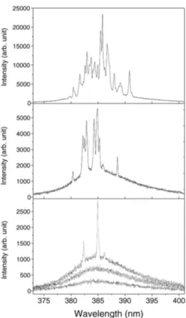
Re-printed from [26]. . . 7 2.3 Spectra of emission from ZnO semiconductor powder
ob-served by Cao et al., while the pump intensity increased from below to above RL threshold (from bottom to top pump en-ergy is 400, 562, 763, 875, 1387 kW/cm2). During this
exper-iment the excitation area was kept the same [26]. . . 9 2.4 Spectra of emission from the rhodamine 640 dye solution
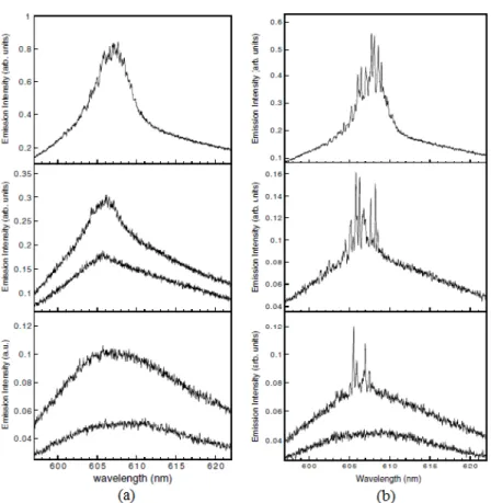
con-taining ZnO nanoparticles corresponding to (a) incoherent and (b) coherent feedback random laser. The ZnO particle density is ⇠ 3 ⇥ 1011cm−3and ⇠ 1 ⇥ 1012cm−3respectively. The incident pump pulse energy is (from bottom to top) 0.68, 1.5, 2.3, 3.3, 5.6 µJ in (a) and 0.68, 1.1, 1.3 and 2.9 µJ in (b) [29]. . . 11 2.5 The spectral-temporal image of the lasing from ZnO powder
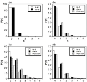
taken by spectrometer-streak camera. The incident pump pulse energy is 4.5 nJ. Reprinted from [13]. . . 14 2.6 The measured photon number distribution of random lasing
from a ZnO pellet (Solid columns) and comparing to the B-E (dotted) and Poisson distribution (dashed) for the same count rate. The ratio between the incident pump intensity and threshold intensity is (a) 1.0, (b) 1.5, (c) 3.0, (d) 5.6. The saturation intensity is assumed as the amount of pump intensity at which the discrete spectral feature appears. Re-printed from [13]. . . 15 2.7 The second-order correlation coefficient as a function of the
ratio of the incident pump intensity Ip to the threshold
in-tensity Ith. Reprinted from [13]. . . 15
2.8 The measured photon number distribution of a random laser emission from dye material for different excitation energy. The data was fitted (lines) by a linear combination of Pois-son and B-E function. Reprinted from [12]. The coherence percentage ↵ = 0, 0.37, 0.49, 0.50 for the excitation energy of E= 1, 4, 7, 12 µJ respectively. . . 16 2.9 Schematic of the experimental setup for (a) spatial coherence
measurement, (b) Michelson interferometry for temporal co-herence measurement. Reprinted from [53]. . . 18 2.10 Visibility (spatial coherence) of the emission as a function
of excitation energy for three different sample concentrations measured by a setup depicted in Fig. 2.9a. An abrupt in-crease in the visibility shows the onset of random lasing ac-tion and represents the threshold, which is in agreement with the theoretical predictions. Reprinted from [53]. . . 19 2.11 (a) Principle of the Raman mechanism due to a F = 1 !
F0 = 2 transition. (b) Experimental transmission spectra recorded with cold85Rb near the F = 3 ! F0= 4 transition
plotted as a function of pump-probe detuning δ. Without pumping, spectrum (1) shows only the atomic absorption. A pump beam of detuning ∆ = 3.8 Γ and intensity 13 mW/cm2,
corresponding to a Rabi frequency Ω = 2.5 Γ , is added to obtain spectrum (2), which then exhibits a Raman resonance in the vicinity of δ = 0. Moreover, the atomic absorption is shifted due to the pump-induced light shift and the absorption is reduced due to saturation. Adapted from Ref. [62]. . . 22 2.12 An example of Raman gain using hyperfine states. Here the
Raman laser makes two-photon transition and generates gain by inducing stimulated emission. The optical pumping laser recycles the atoms and maintains the population inversion between the hyperfine ground states |g1i and |g2i. Reprinted
from Ref. [4] . . . 23 2.13 Threshold for a RL using Raman gain between hyperfine
levels, as a function of the Raman laser parameters (detuning ∆ and Rabi frequency Ω). The optical pumping parameters are ∆OP = 0 and ΩOP = 0.2 Γ. (a) Scheme taking four levels
into account. The lowest threshold is b0cr= 92. (b) Scheme
with five levels involving supplementary scattering from the |2i ! |10i transition (Fig. 2.14). The lowest threshold is
b0cr= 20. Adapted from Ref. [55]. . . 26
2.14 Raman gain scheme used for random lasing in cold85Rb. Sup-plementary scattering is provided by the |2i ! |10i transition.
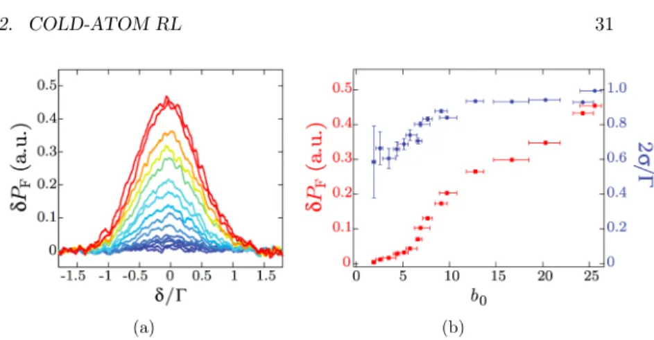
2.16 (a) Supplementary fluorescence around δ = 0 for different optical thickness (same color scale as in Fig. 2.15). The raw data are the same as in Fig. 2.15 but the wings have been subtracted and the signal has been smoothed. (b) A Gaussian fit allows extraction of the amplitude (red squares) and the r.m.s. width σ (blue circles) of the curves shown in (a) as a function of the optical thickness b0. The vertical error bars
are the statistical uncertainties of the fit (not visible for the amplitude) and the horizontal error bars correspond to the fluctuations of b0 on five shots. Adapted from Ref. [4]. . . 31
2.17 (a) |g(1)(⌧ )| and (b) g(2)(⌧ ) for chaotic and coherent light. . . 33
2.18 (a) Schematic diagram of the apparatus for ICM of the scattered light from a cloud of cold atoms. The incoming fluorescence is made partially spatial coherent by a pair of pinholes, Siand Sd, and detected by a photomultiplier tube
(PMT) in a photon counting regime. The required ICMs are performed by the TTL circuitry. (b) Measurements of g(2)(⌧ ) as a function of delay time. The dashed and solid lines are fits assuming two models for the line shape. The circles are meas-urements of an incandescent source for calibration purposes. Reprinted from Ref. [17] . . . 35 2.19 Another scheme of ICM setup used in Ref. [91]. A
single-mode fiber is directed at the reduced image of the cold-atom cloud and the mode-filtered light is led to a photon correlator. SMF: single-mode fiber, FBS: fiber beam splitter, SPCM: single photon counting module, TAC: time-to-amplitude con-verter, and MCA: multi-channel analyzer. . . 36 2.20 Measurements of the second-order intensity correlation as a
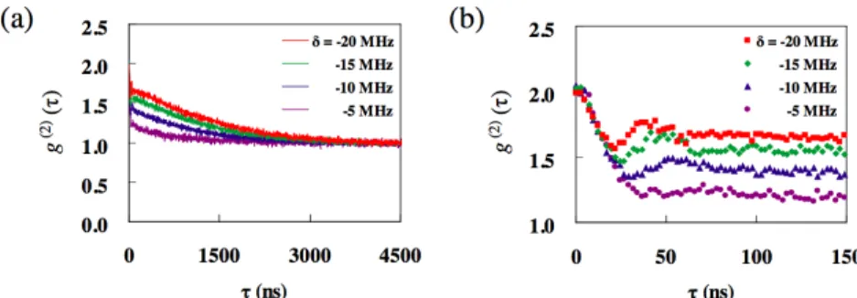
function of delay time for various detuning of the MOT beam. (a) Long-time decay of the correlation function which corres-ponds to the temperature of the cloud. (b) Short-time decay. The short decay time is determined by the lifetime of the atomic excited state. Adapted from Ref. [91]. . . 37 2.21 Schematic diagram of the optical setup to measure the power
spectrum. Reprinted from Ref. [16]. . . 37 2.22 Two power spectra of scattered light from a cold-atom cloud,
normalized to the shot noise level for two different cloud tem-peratures. These spectra contains a narrow and a broad Dop-pler contributions. (a) vrms=pkBT /m = 5 cm/s and (b)
vrms= 3.5 cm/s. Adapted from Ref. [16]. . . 38
2.24 (a) Schematic diagram of the heterodyne detection used in Ref. [15]. (b) Heterodyne spectra with a resolution band-width of 30 kHz at different detuning. The relative vertical scale between the spectra is arbitrary. Reprinted from Ref. [15]. Similar to Fig. 2.22 they referred the narrow part of the spectra to the spatial confinement of the atoms in potential wells. . . 41 2.25 Schematic diagram of the transmission detection used in
Ref. [95] to investigate the EIT effect by performing cross-correlation between two detectors. . . 42 2.26 Photon probability distribution with ¯n = 10 for a (a)
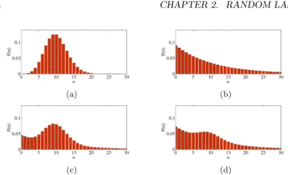
coher-ent, (b) chaotic, (c) partially coherent with coherence percent-age ↵ = 50%, and (d) partially coherent light with ↵ = 20%. 44
3.1 Atomic hyperfine structure of the D2 line of 85Rb and the transitions used for trapping and re-pumping the atoms (Ref.[101]). The cooling laser is tuned to F = 3 ! F0 = 4
atomic transitions with a slightly red detuning (δ = −3 Γ) while the re-pumper laser is tuned to F = 2 ! F0= 3. Level
spacing are not drawn to scale. . . 48 3.2 An overview of the optical setup of the cooling beams. O.I.
stands for optical isolator, λ/2 is half-wave plate, λ/4 is quarter-wave plate, PBS is polarized beam splitter, AOM is acousto-optical modulator, and TA is tapered amplifier. Green lines indicate the feedback lock signals. . . 49 3.3 Schematic optical setup of the re-pumping beams. Two
AOMs are used in this setup. The upper AOM switches on and off (single pass configuration), and the bottom one is being used to scan the frequency of the laser without mis-aligning the beam (double pass configuration). Green line indicates the feedback lock signal. . . 50 3.4 Schematic configuration of the double-pass AOM. This
con-figuration is suitable for scanning the incident beam over a frequency range which is limited by the frequency dependent diffraction efficiency of the AOMs. . . 50
incident probe intensity and the black one corresponds to the transmission of that probe beam through the atoms. Note that the detector gain factor is negative and the range of frequency scan is much larger in the right figure. The flat part at the top of each figure corresponds to the background detection signal when the probe laser beam is switched off. It is clear that the output intensity of the AOM changes a lot during the scan, while on the contrary it is quite stable when the offset lock is used [86]. . . 51 3.6 Hyperfine structure of 85Rb 52P
3/2 level. The frequency of
the transmitted probe beam was scanned by the offset lock-in lock-in a range of [−40 Γ : 20 Γ] durlock-ing 8ms. Γ = 6.06 MHz is the natural atomic linewidth of the rubidium atoms. This range of frequency sweep is much beyond the AOMs working range. . . 52 3.7 A beat-note profile between our DFB and DBR lasers.
Ap-plying a Gaussian fit gives a width (FWHM) of 9.3 MHz for this beat-note profile. . . 53 3.8 (a) The offset lock-in scheme. Details about each electronic
element and how it works are given in the text. (b) A schem-atic diagram of the output voltage of the two high-pass and low-pass RF filters and the result of the subtractor as the error signal. . . 55 3.9 The calibration of the VCO which controls the offset lock.
The feeding voltage of this VCO varies between 1 and 20 V, which corresponds to a range of [487 : 1416] MHz frequency in the output signal. . . 56 3.10 (a) Time evolution of the error signal in the offset lock after
an instantaneous jump of the target frequency at t = 0. Consequently the error signal goes back to zero (±0.1 Γ) at t ⇡ 500 µs, which represents the speed of our offset lock in the range of [−7 Γ : 7 Γ]. (b) and (c) Zoom on the error signals. 57 3.11 Calibration of the RF filter in the offset lock. The vertical
axis represents the output voltage of the subtractor. The input frequency of 253 MHz returns zero output voltage . . . 58 3.12 D2 transition saturated absorption spectrum of the rubidium
vapor. The frequency of master laser is indicated and the fre-quency shift that is needed for the cycling cooling transition of85Rb MOT [105]. . . 59 3.13 Image of our one to six fiber beam splitter. . . 59
3.14 Combination of the cooling and re-pumper beam for the injec-tion into the optical fiber. Note that, because of the polarized beam splitter (PBS), the polarization of the MOT beam and the re-pumper is perpendicular at the fiber injection. . . 60 3.15 (a) The intensity profile of a trapping beam just before
propagating through the vacuum chamber. The beam was intercepted by a white paper and the image of it was taken by a camera. Calibration of this camera gives 0.173 mm for each pixel size of the image and this image contains 360⇥360 pixels. (b) One dimensional spatial profile of the beam along x-axis and (c) y-axis and their Gaussian fits, which show a waist size (width at 1/e2) of ⇡ 29 mm and ⇡ 34 mm respectively. . . 61
3.16 Absorption image of (a) a standard MOT realization (δimg=
0 Γ, b0⇡ 5) and (b) after applying the dark MOT compression
to it (δimg= −2 Γ, b0= 22). Please note that in order to fit
the image of MOT into the frame, a short loading time was used. In practice we are able to produce bigger and optically thicker MOT and dark MOT (up to b0 = 150). The size of
standard MOT compressed from 2.9 mm to 0.9 mm for dark MOT. . . 63 3.17 Calibration of an AOM by changing the voltage input of the
VCO which feeds that AOM, in order to vary the intensity of the diffracted beam. The voltage controls the amplitude of the VCO modulation and hence it changes the efficiency of the diffraction in the AOM. This calibration has been normalized to the maximum intensity of the diffracted beam. . . 63 3.18 Optimizing the re-pumper intensity and DMOT duration in
order to have maximum optical thickness. (a) b0 as a
func-tion of the reduced re-pumper intensity during 35 ms. (b) b0
as a function of DMOT duration with a reduced re-pumper intensity to 2% of its initial value. The total initial re-pumper intensity was ⇡ 5 mW. Each point is the average of 10 realiz-ations and the errorbars are the standard deviation of them. . 64 3.19 Experimental transmission curves for three different b0 =
0.9, 8.3, 77. . . 66 3.20 Measured transmission (light gray) of a probe through a MOT
with small optical thickness, b0 = 0.27. Applying a
convolu-tion fit based on Eq. 3.10 we estimated 3.6 MHz for the probe laser linewidth. . . 67 3.21 Time sequence of a typical absorption imaging process. In
this sequence, first the MOT is loaded, then compressed to achieve higher optical thickness, then by applying molasses phase, the temperature is modified, and finally the absorption image is taken. . . 69
3.23 Absorption images of dark MOT taken after different TOF durations. δimg was chosen to keep b(δ) ' 1, (δimg =
−3, −2.5, −1.8, −1, −0.3 Γ from left to right respectively). From this time-lapse one can estimate the gravity of Earth g. 72 3.24 Decay of the magnetic field measured by a Gauss-meter (a)
and the current in the coils (b) after switching off the netic gradient. The normalized decay signals of both mag-netic field and the current are compared (c). It is realized from the figure that an approximately 2ms delay time is needed for the I and B-field to get to zero with 2% error. . . 73 3.25 Time of flight measurements of a dark MOT with Nat⇡ 1010
and b0 ⇡ 100, (a) in the x-dimension and (b) in the
y-dimension. The slope of each plot is a measure of kBT
m .
Con-sideringkB
m = 97.9188m
2
s2K the above plots show a temperature
of about 110 µK for the MOT. . . 74 3.26 b0 as a function of TOF duration. The errors correspond to
the statistical variations in the measured optical thicknesses. A fit, based on the relation b0 / N/σ2(t), is applied (blue
line) to estimate the optical thickness at different TOF. . . . 75 3.27 Fluorescence signal representing the loading of a MOT. The
detuning of the cooling beam is δM OT = −3 Γ. An
exponen-tial fit (Eq. 3.25) gives γ−1= 1.2 s (red dashed line). . . . 76
3.28 The image of the valve which connects the Rb reservoir to the vacuum chamber. . . 77 3.29 Rubidium transmission spectra from a reference cell and
the vacuum chamber. Eq. 3.28, (a) shows a pressure of ⇡ 10−7mbar, while after reducing the pressure to 10−8mbar
in (b) the absorption signal in the vacuum cell was not strong enough so that we could not use Eq. 3.28 to estimate pressure. 79 3.30 A snapshot of the standard MOT produced in the vacuum
chamber (with a length 10 cm) in our experiment. . . 80 4.1 Schematic of the gain curve measurement. . . 84 4.2 The gain curve recorded at the AC output of a
trans-impedance photodiode accompanied by an amplifier. . . 85 4.3 Typical intensity noise SP of the DFB laser as a function
of Fourier frequency fn, obtained with a mean laser power
of 80µW. The gray vertical lines indicate specific frequencies which is used to extract the noise power as a function of optical power in Fig. 4.4. . . 86
4.4 Power spectral density SP of the DFB laser intensity
fluctu-ations as a function of the mean power at different frequen-cies. The data are well fitted by a square law (solid line with fn= 1 MHz) corresponding to a classical noise. The dashed
line corresponds to the shot noise level calculated by Eq. 4.3. 87 4.5 The intensity fluctuations of a laser diode as a function of
the mean incident optical power at fn= 400 kHz. The noise
power scaled linearly up to ⇠ 100µW which describes the shot noise limited domain, while above this power, noise power is scaled quadratically which shows classical noise domain. . . . 87 4.6 Relative intensity noise for the DFB laser diode. The mean
power is about 80µW. . . 88 4.7 Beat-note setup to measure laser line shapes. Two lasers
are injected into a 50:50 fiber coupler. The beat-note signal is detected by a fast photodiode (PD). The signal is finally analyzed with a spectrum analyzer. . . 89 4.8 Beat-note signal PSD between the DFB laser and the
TOP-TICA laser. The center of the spectrum has been shifted to the origin. Since the TOPTICA laser has a much smaller linewidth than the DFB laser one, it can be treated as a ref-erence laser and the PSD mainly corresponds to the optical spectrum of the DFB laser. The central part can be fitted by a Gaussian (dashed line) with a FWHM ∆⌫BN' 3 MHz,
and the wings are well fitted by a Lorentzian (solid line). In-set: zoom on the Gaussian part of the optical spectrum. Red curve: beat-note signal PSD. Dashed curve: Gaussian fit. . . 90 4.9 The central parts of the beat-note PSD profiles for the (a)
DFB and Toptica, (b) DFB and SYRTE and (c) SYRTE and Toptica laser diodes and their Gaussian fits. All the beat-notes were shifted to the origin. The fits give FWHM = 0.49 Γ, = 0.52 Γ, and = 0.18 Γ respectively. Each beat-note are recorded after 100 averaging. The resolution bandwidth (RBW) and video bandwidth (VBW) were set on 1 kHz and the spectrum analyzer span was 10 MHz. . . 92 4.10 The beat-note signals between a DFB and a DBR lasers
fre-quency locked, with (triangle marks) and without (square marks) a low-pass RC filter at the output of the laser driver with a cutoff frequency at fc = 2.7 kHz. Gaussian fits
(purple and green respectively) were applied to measure the linewidth. The RC filter reduces the electronic noise in the current driver and narrows down the beat-note linewidth from 6 to 4 MHz. . . 94
we used synthesizer to drive the AOM, then the beat-note taken by the setup (a) is compared with the one taken by the setup (b) (Fig. 4.13). . . 95
4.12 The effect of the electronic noise in the driver of an AOM on the beat-note linewidth of the DFB laser. In this meas-urement, the self beat-note profiles of the DFB laser with one beam which is diffracted by an AOM controlled by a homemade VCO (blue line) and by a Rohde & Schwarz syn-thesizer (red line) were recorded. The scheme of the meas-urement is illustrated in Fig. 4.11a. The beat-notes were shifted to the origin. The video bandwidth (VBW) and the resolution bandwidth (RBW) were set at 30 Hz with a span of 100 kHz on the spectrum analyzer and the beat-notes were recorded after 300 samples averaging. . . 96
4.13 The effect of the tapered amplifier on the beat-note linewidth of the DFB laser. In this measurement, the self beat-note profiles of the DFB laser without (dashed black line) and with (solid red line) a tapered amplifier were recorded. An AOM driven by a synthesizer was used to make 100 MHz frequency shift in the beat-note. The basis of the measurement was presented in Fig. 4.11b. Both curves are almost the same and thus there is no broadening due to the amplifier. The VBW and RBW were set at 10 Hz with a span of 100 kHz on the spectrum analyzer and the beat-notes were recorded after 100 samples averaging. . . 96
4.14 Schematic diagram for frequency to intensity conversion using an optical frequency discriminator. . . 98
4.15 (a) The transmission spectra of the rubidium atoms (red curve) while the frequency of the laser was scanned by a trian-gular voltage (green curve) produced by a function generator and injected into the laser driver. By changing the amplitude of the voltage signal we can change the range of frequency scan. In the atomic spectrum,87Rb F = 2 ! F0= 2, 3 and 85Rb F = 3 ! F0= 4 transitions with a frequency distance
of 1.26 GHz are marked which corresponds to a conversion of 1.19 V.GHz−1. (b) Transmission of the Fabry-Perot
cav-ity by scanning the frequency of the laser via a triangular voltage. The transmission is plotted as a function of laser frequency scan thanks to the previous conversion factor. The space between two consecutive transmission peaks is the free spectral range of the cavity (∆⌫F SR= 980 MHz). Applying a
Lorentzian fit also to one of the peaks gives a cavity linewidth of ∆⌫c= 73 MHz and thus the finesse is F = 13. . . 100
4.16 (a) Schematic of the frequency noise power spectral density (FNPSD) measurement using a Fabry-Perot cavity as a fre-quency discriminator. (b) A typical intensity transmission from a Fabry-Perot cavity(gray line). A Lorentzian fit can be applied to this experimental curve to measure the cav-ity linewidth ∆⌫c (red dotted line). The derivative dTc/d⌫L
(blue dashed line) is also demonstrated to show the optimum frequency to intensity noise conversion, occurring at half max-imum of the transmission where |dTc/d⌫L| is maximum. . . . 101
4.17 Frequency noise PSD for the DFB and the TOPTICA lasers. 101
4.18 FNPSD for the DFB and the TOPTICA lasers and geomet-rical approach with the β-line to estimate the laser linewidth. Dark grey area: area which contributes to the TOPTICA laser linewidth. Light grey area: area which contributes to the DFB laser linewidth. . . 104
in the MOT and compressed to achieve high density during ti.
Then the trapping system switches off and atoms are released. Two probe pulses are applied during tp= 1.2 ms, after a time
of flight of tT OF = 4 ms. The first pulse provides the
trans-mission through the atomic cloud, and the second one allows us to measure the incident intensity without atoms in order to calculate the normalized transmission for each cycle. The atoms are removed by applying the MOT beams at resonance during tpush = 6 ms between the two probe pulses. For the
PSD measurements the time window of the oscilloscope is set tpause = 200 µs after the beginning of the first probe within
tosc= 100 µs. . . 106
4.20 The value of transmission noise from a cloud of cold atoms with optical thickness b0 = 19 at fn = 500 kHz taken with
different laser detuning δ (dots), compared to the square of discriminator slope (solid gray line). . . 107 4.21 (a) Transmission through an atomic cloud as a function of the
laser detuning and for three different optical thicknesses. (b) Frequency discriminator as a function of the laser detuning. These curves are obtained from the derivative of the trans-mission fits and will be used for the frequency intensity noise conversion. . . 109 4.22 Laser transmission noise PSD SIndivided by the square of the
discriminator slope D2="dT
a/d⌫L#2, measured using a cold
atomic cloud as a frequency discriminator. For low Fourier frequencies, Eq. 4.37 is valid and the curves thus correspond to the laser FNPSD. The FNPSD measured with the Fabry-Perot cavity is plotted in grey. The β-line corresponds to the dashed line. . . 110 4.23 Schematic of the phase modulation model by treating the
broad optical spectrum wings as frequency sidebands. For more information see text. . . 112 4.24 Examples of phase shift φ(δ) in radian and normalized
trans-mission T (δ) = exp [−↵(δ)] as a function of laser detuning δ, for three different cloud optical thickness b0= 5, 20 and 50. . 114
4.25 The simulation based on Eq. 4.61 for different optical thick-nesses b0 and laser detuning δ as mentioned in the figures
legend. The optical thickness and detuning has been chosen to keep almost the best frequency to intensity noise conver-sion due to D2. . . 116
4.26 Zoom at high frequencies of laser transmission noise PSD ST
divided by the square of the discriminator slope D2 using a
cold atomic cloud with an optical thickness of b0 = 19 and
for three different laser detunings. . . 117 4.27 Green solid line: laser transmission noise PSD ST divided by
the square of the discriminator slope D2 = (dT
a/dδ)2 using
a cold atomic cloud with an optical thickness of b0= 19 and
a laser detuning of δ = 3. Dashed line: S⌫L,th/D
2 calculated
using Eqs. 4.59 and 4.60 assuming a white frequency noise. . 118 4.28 Comparison of (a) calculated Eq. 4.61 and (b) experimental
laser transmission noise PSD for optical thickness b0 = 19
and detuning δ = 2, 3, 4, 5. . . 119 4.29 Comparison of (a) calculated Eq. 4.61 and (b) experimental
laser transmission noise PSD for optical thicknesses b0 = 19
and b0= 51 and detuning δ = 3. . . 120
4.30 Points: experimental frequency position of the bumps (circles: first bump, triangles: second bump) observed in the frequency noise PSD, obtained with the cold atomic cloud, as a function of the laser detuning. Solid line: calculated frequency position of the first bump. Dashed line: calculated frequency position of the second bump. . . 121 4.31 An intuitive picture for the origin of the bumps in a
trans-mission noise PSD. below, the laser optical spectrum at its carrier frequency is supposed to encounter a cloud of cold atoms with a transmission function T as described by the black curve in the center of the figure. The width of trans-mission curve scales aspb0. This means that by increasing
b0, the width of transmission function increases proportional
topb0. In the top a relevant transmission noise PSD is
de-picted. The bumps represent two group of sidebands in the laser optical spectrum which encounter two different sides of the transmission spectrum at about maximum frequency-to-intensity conversion. We observed that the space between two bumps changes proportional topb0. . . 122
4.32 The calculation of (a) A2 based on Eq. 4.59 and (b) A02in Eq. 4.69 for optical thicknesses b0= 5, 20, 50 with the same
detuning δ = 3Γ. Note that A2 has an overall behavior as
1/f2
nat low frequencies while A02is nearly flat. . . 123
4.33 (a) The FNPSD and (b) the transmission intensity noise cal-culated based on amplitude modulation model in Eq. 4.72 and 4.70, for optical thickness b0= 19. . . 123
3Γ. Experimental data (green), compared with theoretical simulation based on phase modulation (pink) and amplitude modulation models (blue). . . 124 4.35 Transmitted intensity noise PSD ST calculated based on
phase and amplitude modulation models in Eqs. 4.60 and 4.70 at a given frequency (a) fn = 1 MHz and (b) fn = 30 MHz
while the detuning δ is scanned between −5 to 5 Γ. The optical thickness b0 = 19. The noise created by phase
ulation is larger than the one generated by amplitude mod-ulation. At high frequencies, the M-shaped spectrum corres-ponding to phase modulation is distorted. This might be due to the complicated bumps and dips features in the spectrum and the dependence of their positions to the different detunings.125 4.36 (a) Transmitted intensity noise PSD ST for different optical
thicknesses b0= 3, 7, 15, 20, 30 and 50. Note that here the
in-tensity noise PSD after transmission is not normalized by the derivative of the frequency discriminator. (b) The noise power at fn = 1 MHz (dashed blue line) and fn = 40 MHz (solid
orange line) as a function of b0computed by the phase
modu-lation model. The blue plus and orange star symbols corres-pond to experimental measurements. The experimental data confirms the prediction from computations. The deviation between computation and experimental data at fn= 40 MHz
could be due to the noise floor of our detection system. In this measurement, b0was modified by applying different TOF
Comparing the values of |g (⌧ )|, g
P(n) of different types of light. ”P” and ”B-E” stand for Poisson and Bose-Einstein distribution respectively. . . 13 2.2 Comparing the lowest threshold in different gain mechanisms.
Considering this table, the Raman gain between the hyperfine ground states with additional scattering is the most feasible mechanism for generating cold-atom RL. In our lab we are able to make a cold-atom cloud with the optical thickness of b0⇠ 10 − 200. . . 27
2.3 Summarizing different known techniques for studying the noise properties of the light from the cold atoms. FP: Fabry-Perot cavity, ICM: intensity correlation measurement, SNR: signal to noise ratio, and LO: local oscillator. . . 43 3.1 Comparing different MOT properties before and after solving
the problem in the performance of the ionic pump. After solving this problem we achieved lower vacuum pressure (10−8mbar). . . . 79
4.1 Table of notation used in the following chapter. . . 81 4.2 Beat-note and deduced laser linewidth, compared to the
ex-pected values. The uncertainties are statistical errors taken at 1σ. . . 93 4.3 Different frequency noise component, classified based on their
frequency functionality. . . 97 4.4 Frequency noise standard deviation σ⌫L for the TOPTICA
and the DFB lasers calculated by Eq. 4.23. . . 100 4.5 Laser linewidth measured by the β-line approach and
com-pared with the values from the beat-note measurements. . . . 104 4.6 DFB laser linewidth measured by different techniques. . . 110
Random laser
The idea of random lasing was first proposed by Letokhov who considered the propagation of light in the presence of amplification or gain in a mul-tiple scattering medium [1]. In such a situation, mulmul-tiple scattering increases the effective path length in the gain medium and thus enhances light amp-lification. Letokhov developed a theoretical model based on the diffusion equation and he defined a threshold on the system size above which the amplification in the volume overcomes losses at the surface of the medium, leading to an exponential increase of the light intensity trapped in the me-dium and hence of the subsequent emitted light [1, 2]. This is very similar to the principle of a laser, which starts oscillation when the gain produced by the amplifying medium overcomes the cavity losses. Here, the cavity is replaced by radiation trapping due to multiple scattering [3], and therefore the spatial and spectral lasing modes are different.
Random laser has been observed in many different media including laser dyes, semiconductor powders, ceramics, nanostructured and non-nanostructured thin films, etc [2]. Recently cold-atom random laser was also observed in our team [4] by investigation of the level of fluorescence from the atoms. The rubidium atoms are cooled in a magneto-optical trap (MOT). Here the cold atoms provide both gain and multiple scattering. In this system, a two-photon Raman transition between the hyperfine atomic levels provides gain. Considering the hyperfine structure of the rubidium atoms, the frequency of the laser which makes this Raman transition can be tuned, where the scattering of the laser by the atoms is minimized and simultaneously the scattering of the induced gain is maximized.
State-of-the-art random lasers are usually based on pulsed excitation of condensed matter systems and quasi cw operation of random lasing in dilute atomic vapors had not been realized prior to our recent study [4].
Motivations
Existence of a natural laser emission has long been an open question for scientists. Astronomical observations in the microwave domain have led to the discovery of anomalously bright emission lines from molecules in stellar atmospheres [5]. Moreover spectroscopic data from the atmosphere of planet Mars and planet Venus revealed an extraordinary emission line in infrared
(IR) domain (λ ⇠ 10 µm) from CO2 molecules [6, 7]. Much later, this
type of emission was also observed in stellar atmospheres in the far IR [8]. This amplification by stimulated emission in Mars was first observed by Charles Townes’ team [6], and later identified as a ”natural laser”. It was used later as a diagnostic probe of the temperature and wind patterns on Venus [9]. Due to the low densities of the lasing species in the mesosphere and thermosphere of Mars the gain is low, comparable to single-pass gains in some earth based CO2lasers [7]. The low gain though is partly compensated
by the extremely large volumes of active lasing medium.
It should be noted here that astrophysicists often call ”lasers” what a laser physicist would describe as amplification, or Amplified Spontaneous Emission (ASE) [10].
Owing to the huge amount of gain medium in combination with very intense sun light in the Venus atmosphere, scientists in NASA proposed an ambitious project [11]. They designed some satellites carrying mirrors to be located around the Venus atmosphere in order to enhance natural lasing emission for interstellar communication. This was a part of the program ”search for extraterrestrial intelligence” (SETI). However this proposal was never implemented.
Discriminating the random laser emission among all the other sources of radiation from an astronomical object for instance, requires well-developed knowledge and measurement techniques. In particular, for the case of cold-atom random lasing developed at INLN, it is very difficult to resolve random laser spectrally and spatially among all the other emitted or scattered light. In fact there are at least four spectral lines which are separated by 10s of MHz and random laser emission has to be resolved amongst them.
Temporal and spatial coherence are strong tools which can potentially help to better understand and also to classify an unknown source of light emission. Several theoretical and experimental efforts demonstrated that, in general, random lasing emission is partially coherent [12, 13]. However its coherence is usually less compared with the conventional lasers [14]. These coherence properties depend on the experimental parameters and material used, and could be different from one experiment to the other. However, due to very complicated mechanism of multiple scattering, the coherence of random laser is not completely known and it seems an open question.
The long term goal of this work is to characterize the temporal coherence properties of the cold-atom random laser. This can help to distinguish the lasing modes and threshold condition. The coherence of the scattered light through the cold atoms in the single scattering regime has been already investigated in some experiments [15, 16, 17], which provides us with solid applicable coherence measurement techniques and physics beyond it. Nevertheless to approach step by step coherence measurement and analysis
scattered light. Finally, the impact of adding gain has to be taken into account below and above the lasing threshold.
Thesis outline
The content of this thesis is organized as follows. In chapter 2 we intro-duce the ”random laser” phenomena. The results of some theoretical and experimental research on the coherence properties of random laser are sum-marized briefly. Then the prior observation of cold-atom random laser is also reported, and some possible experimental techniques for studying its coherence properties, which can be possibly applied in cold-atom random laser, are introduced.
In chapter 3, we explain the current status of our85Rb MOT experiment.
Furthermore some experimental and technical informations will be provided about characterizing and modifying the important physical parameters such as temperature, density, and optical thickness.
Finally, in chapter 4 we characterize the lasers used for probing the cold atoms. These properties include laser line shape and linewidth, intensity and frequency noise. Then, using those information, we study the noise power spectral density (PSD) of a laser beam transmitted through the cold atoms. In order to understand the noise features, two models based on phase and amplitude modulation are introduced and compared with the experimental results.
Two fundamental ingredients of a conventional laser are an amplifying ma-terial, which provides optical gain, and an optical cavity that partially traps the light and induces feedback. When the total gain overcomes the losses, the system reaches a threshold and lasing occurs. The mode properties of a laser are determined by the cavity, i.e. the frequency and directionality of the output light. Similar to a conventional laser, random lasers are based on the same principles, but here it is multiple scattering that induces feedback and determines the lasing modes instead of the cavity (Fig. 2.1). The term ”random laser” was introduced and suggested in 1995 by Wiersma et. al. [18].
Figure 2.1 – Comparison between a conventional laser (a) and a random laser (RL) (b). In a regular laser the light is captured in the optical cavity and passes through the amplifying material several times. The gain amp-lification in this situation can be sufficiently large for the onset of lasing. Although the optical cavity is absent in the RL, the photon lifetime in the amplifying material due to the multiple scattering can be long enough that the amplification corresponding to the stimulated emission becomes efficient and the lasing begins in random directions [19].
Multiple scattering is a well-known phenomena, which occurs almost in all the opaque optical materials. The resemblance between a human tissue and a white paint is that the light propagating in both media undergoes multiple scattering. The propagation of light in such a system can be de-scribed as a random walk, like the process which happens to a photon inside
the core of sun before it escapes. This type of propagation can be modeled and studied by the diffusion equation. In 1968 Letokhov investigated the diffusion of light due to multiple scattering in the presence of gain and he found a critical situation where the amplification of light gets larger than losses and the so-called self-generation of photons occurs [1]. Letokhov’s prediction was observed for the first time in 1994 by Lawandy et al. [20].
2.1
Random laser (RL)
2.1.1
Introduction
Although in the conventional lasers multiple scattering is usually considered as a detrimental effect, which removes lasing photons from the laser cav-ity mode, this effect combined with the gain can establish lasing. Multiple scattering increases the propagation length of a photon diffusing in that me-dium. This enhances the light amplification related to stimulated emission. Of course the mode properties are different from the lasers with cavity.
This type of lasing was first discussed theoretically by Letokhov. He showed that for light diffused in a medium in the presence of gain, the total amplification is scaled with the volume of the system whereas the losses are proportional to the total surface [1]. He predicted a threshold where the gain overcomes the losses and consequently the intensity of light increases with time and diverges. In the case of frequency dependent gain, the diffusion model also predicts narrowing in the spectrum of the emission above the threshold with a maximum at the same frequency as the maximum of the gain.
To describe the scattering process, two basic lengths are defined. The mean free path, `sc, which is the average distance that light travels between
two consecutive scattering events, and the transport mean free path, `t,
which is defined as the average distance that the incident light propagates in the medium before its direction gets randomized. These two length scales are linked by
`t=
`sc
1 − hcos(✓)i, (2.1)
where ✓ is the scattering angle.
To characterize the light amplification due to stimulated emission, the gain length `g is defined as the path length over which the intensity of the
light is amplified by a factor of e, and the amplification length `ampwhich is
the rms average of distance from the beginning to the ending point for paths of length `g [2]. When the medium is transparent and homogeneous, light
travels in a straight line and thus `amp= `g, whereas in a strongly scattering
regime where a photon diffuses in the medium, `amp=
p
Dt, where D is the diffusion coefficient and for a 3-dimensional system is D = v`t/3, where v is
Figure 2.2 – Coherent backscattered light cone from ZnO powder film. Re-printed from [26].
the transport velocity of light. t also can be written as t = `g/v, thus
`amp=r `g`t
3 . (2.2)
Generally three regimes of light transport are considered in a 3D dis-ordered medium
• The ballistic regime, `t≥ L
• The diffusive regime, L , `t, λ
• The localization regime, ke.`sc⇡ 1
where L is the size of the medium and ke= k0/n is the effective wave-vector
and k0 is the wavevector and n is refractive index [21]. Experimentally
`t can be measured from the angular width of the backscattered cone of
light in a coherent backscattering (CBS) experiment [22, 23, 24, 25]. In this experiment the angle of the backscattered light cone (Fig. 2.2) at the full-width at half-maximum (FWHM) is written
∆✓ ' 0.7 ke`t
. (2.3)
2.1.2
Letokhov photonic bomb
In the diffusive regime, the diffusion of photons in a medium with a uniform and linear gain is described by
@W (~r, t)
@t = Dr
2W (~r, t) + v
`g
where W (~r, t) is photon energy density, D is the diffusion coefficient of the photon. A general solution to Eq. 2.4 is
W (~r, t) =X
n
an n(~r)e−(DB
2
n−`gv)t, (2.5)
where anare arbitrary constants and depend on the initial and boundary
conditions, Bnand n(~r) are respectively eigenvalues and eigenfunctions of
the equation
r2
n(~r) + Bn2 n(~r) = 0, (2.6)
which is obtained by substituting Eq. 2.5 into Eq. 2.4 and using modal decomposition. The boundary condition in such a system is defined as
n(~r)|~r=ze = 0 at distance ze, which is known as the extrapolation length
and quite often is much smaller than the physical dimension of the random medium and hence it can be approximated as n = 0 at the boundary of
the medium.
Eq. 2.5 shows a change from an exponential decay to an exponential increase in time when the system crosses the threshold
DB12−
v `g
= 0, (2.7)
where B1is the lowest eigenvalue. The values of Bndepend on the geometry
of the medium, for example in a spherical shape with diameter L, Bn =
2⇡n/L, and for a cube shape with side length L, B1=p3⇡/L [2]. Regardless
of the shape of the scattering medium, order of magnitude for B1 is 1/L.
For a spherical shape, Eq. 2.7 results to a critical size for the system Lcr= 2⇡
r `t`g
3 . (2.8)
If the gain length `gand the transport length `tare kept fixed, for a size of
the medium above a critical value, W (~r, t) starts growing exponentially with time. Because of the similarity between this self-generation of the photons and the neutron multiplication in a nuclear bomb, this process is sometimes referred as a photonic bomb.
Although this model predicts a divergence for the light intensity, because of the gain depletion no explosion occurs. The gain begins to deplete quickly and consequently `gincreases. By considering the gain saturation, Letokhov
predicted a damped oscillation (pulsation) in the transient process of the generation. He also calculated the emission linewidth. The main limiting factor for the width of the lasing spectrum in the stationary regime comes from the spontaneous emission. Otherwise the Doppler effect from moving scatterer particles also induces some noise in the photon frequency [1].
Fig. 2.3 demonstrated the spectral features of RL emission from semi-conductor powder while the pump intensity increased.
Figure 2.3 – Spectra of emission from ZnO semiconductor powder observed by Cao et al., while the pump intensity increased from below to above RL threshold (from bottom to top pump energy is 400, 562, 763, 875, 1387 kW/cm2). During this experiment the excitation area was kept the
2.1.3
Coherent and incoherent feedback
Classifying random laser (RL) into coherent and incoherent feedback lasing categories, has been debated in the past two decades. It was initially believed that as the density of scatterers increases, the probability that the light comes back in closed loops during its propagation increases. That means the interference of light in this situation has to be taken into account. When the gain in such a loop exceeds the loss, laser oscillation can occur. The required constructive interference due to the total phase shift along the loop determines the frequency of oscillation. This is known as RL with coherent feedback [26, 27, 28].
The incoherent feedback can be interpreted in terms of modes. Instead of individual high-Q resonances there appear a large number of low-Q res-onances which spectrally overlap and form a continuous spectrum. This corresponds to the occurrence of incoherent feedback. The absence of co-herent feedback means that the cavity spectrum tends to be continuous, i.e., it does not contain discrete components at selected resonant frequencies [2]. By increasing the density of scatterers Cao et al. [29] observed the transition from incoherent to coherent feedback random laser (Fig. 2.4).
One main difference between the two types of feedback is that, in the incoherent one the interference effect is negligible, the photon is diffused and makes random walk in the disordered medium and mathematically the in-tensity can be analyzed by a diffusion equation to explain the lasing. Indeed this is at the heart of Letokhov’s model. Whereas in the coherent feedback lasing, the interference effect cannot be neglected and is essential, so the electric field has to be studied instead of the intensity. The picture of closed loops is intuitive but naive. In general light can go back to its origin in many different paths, and all the backscattered light interferes and determines the lasing. Thus the coherent feedback RL is a randomly distributed feedback laser.
In order to develop a model which describes the coherent RL emission, instead of the diffusion equation for the light intensity, the Maxwell equa-tions for the electro-magnetic fields should be used [30]. Several theoretical models have been already introduced, such as time-dependent theory [31], the collective modes of resonant scatterers [32], the prelocalized modes in diffusive media [33], the Anderson model [34], etc.
2.1.4
Coherence properties of random lasers
Temporal coherence and photon statistics
One important feature of the laser emission is its temporal coherence. The-oretical studies predicted that the random laser above threshold could be a coherent light [35] and its photon statistics could be very similar to those of a conventional laser.
Figure 2.4 – Spectra of emission from the rhodamine 640 dye solution con-taining ZnO nanoparticles corresponding to (a) incoherent and (b) coherent feedback random laser. The ZnO particle density is ⇠ 3 ⇥ 1011cm−3 and
⇠ 1 ⇥ 1012cm−3respectively. The incident pump pulse energy is (from
bot-tom to top) 0.68, 1.5, 2.3, 3.3, 5.6 µJ in (a) and 0.68, 1.1, 1.3 and 2.9 µJ in (b) [29].
![Figure 3.1 – Atomic hyperfine structure of the D2 line of 85 Rb and the transitions used for trapping and re-pumping the atoms (Ref.[101])](https://thumb-eu.123doks.com/thumbv2/123doknet/14550346.536835/85.918.281.705.268.821/figure-atomic-hyperfine-structure-transitions-trapping-pumping-atoms.webp)


