Fundamental-driven and Tactical Asset Allocation: what really matters?

Fundamental-driven and Tactical Asset Allocation: what really

matters?

Jean-François Boulier* and Maria Hartpence**

March 2004

Cahier de recherche n° 2004-06

Abstract

Asset allocation contribution to ex-post performance is of primary importance. Nobody denies its role, yet the subject of allocating assets remains controversial. To some contenders, the added value stems only from strategic asset allocation which aims at providing the long-term average exposure to the selected asset classes. On the other hand, proponents of active management have introduced several forms of tactical asset allocation.

In this paper, we will go a step further by distinguishing between 1) long-term strategic asset allocation, 2) medium-term strategic or fundamental-driven asset allocation and, finally, 3) tactical asset allocation. “Fundamental-driven” refers to the inclusion of slow business cycle components and structural changes in the economies. “Tactical”, by contrast, exploits short term transitory mispricings in the markets. When one takes into account various types of information, it leads to various conditioning processes and thus to the three levels of asset allocation mentioned above. As an example, we illustrate how models can be used for computing the asset expected returns related with different asset allocation levels. We show that error correction models are particularly useful in this context. Finally, using these concepts, we present simulations of two actively managed balanced portfolios – equity and bonds – in the US and Europe. The simulation results show the added value of allocation either Fundamental-driven or Tactical on the portfolios’ return.

* Head of Euro Fixed Income and Credit CA-AM, CLAM

Crédit Lyonnais Asset Management, 168 rue de Rivoli, 75044 Paris cedex 01 Telephone : + 33 1 42 95 97 58 Fax number : + 33 1 42 95 75 18

e-mail : jean-francois.boulier@creditlyonnais.fr

** Head of Investment Research - SINOPIA Asset Management

SINOPIA Asset Management, 66 rue de la Chaussée d’Antin, 75009 Paris Telephone : + 33 1 53 32 52 78 Fax number : + 33 1 53 32 52 20 e-mail : maria-laura.hartpence@sinopia.fr

portfolio with broad asset categories (such as stocks, bonds, cash, real estate, ...) depending on the investment horizon, objectives, constraints and risk tolerance of the investor. By “optimal” we mean a portfolio that maximizes the expected return/risk ratio for the constraints defined by the investor.

This process can be performed on any portfolio with two or more “assets”, however the term “asset allocation” most commonly refers to allocation of “asset classes”, the single decision that has the greatest impact on the portfolio’s return.

A distinction between levels of asset allocation can be made. Most often people refer to strategic asset allocation, which is based on long-term forecasts for expected returns, volatility and correlations between financial assets, and tactical asset allocation, founded on short-term forecasts.

In this paper, we will go a step further by distinguishing between 1) long-term strategic asset allocation, 2) medium-term strategic asset allocation, which we will call “fundamental-driven asset allocation” and finally, as before, 3) tactical asset allocation. We will see that each of these asset allocation levels are conditional upon different types of information, mostly related with economic cycles and market asset prices, as these factors are at the origin of expected asset returns. We will show that the fundamental-driven asset allocation and tactical asset allocation, which are both deviations from the long-term strategic asset allocation, are both sources of performance.

This paper is organized as follows. The first part will describe the determinants of the three levels of asset allocation defined above.

The second part of this paper will explain how models can be used for computing the expected asset returns related with different asset allocation levels, by specifically conditioning these expected returns to different types of information. We shall show that error correction models are particularly useful in this context.

Finally, part three will apply these concepts for building expected returns for the bond and equity US and European markets, using two stylized valuation models for each asset class. We will present simulations of an actively managed global balanced

will repeat the exercise for the European market. The simulation results will show the strong positive impact of tactical allocation on the portfolio’s return.

I.

Levels of asset allocation

I.1. Long-term strategic asset allocation

The first and most important choice that a private or institutional investor must do when organizing his portfolio is the long-term strategic asset allocation. Long-term strategic asset allocation is the choice of the proportion of and within asset classes that the investor wishes to hold on the long run. This decision will be the result of the investor’s goals and constraints, as well as its risk and return expectations for the portfolio assets, for the investment horizon, usually of 10 to 25 years.

Strategic asset allocation may materialize in a

constant mix of and within different asset classes.

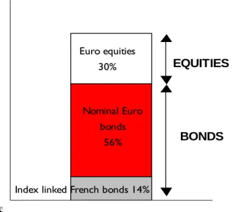
Figure 1 exhibits an example of a long-term strategic asset allocation for a French complementary retirement scheme fund, with 70% Euro bonds – where 20% corresponds to French index linked bonds – and 30% to Euro equities. In some instances a known public benchmark can be implemented in the strategic portfolio.

Figure 1

Long-term strategic allocation of a hypothetical French complementary retirement scheme fund

In the French fund example, the European equity segment may be represented by the MSCI Euro

Euro equities 30%

Nominal Euro bonds

56%

Index linked French bonds 14%

EQUITIES

index. In this case, although the strategic stock proportion to be held in the long run is 30%, the weights of the local European markets may change over time, following the time varying composition of the MSCI Euro index.

As mentioned above, the long-term strategic asset allocation choice derives from a certain number of parameters. A well-known answer for the strategic allocation decision is the Markowitz (1952) mean-variance analysis, applied to a world of risky assets and a risk-free asset. In this framework, for a given choice of risky asset classes, say, stocks and bonds, the first step is to calculate the efficient frontier: the set of optimal portfolios in terms of expected returns and risk, i.e. the different combinations of stocks and bonds that maximize the expected return of a portfolio for different risk levels. The theory shows that, given the existence of a risk-free asset, there is one optimal portfolio of risky assets, which should be combined with the risk-free asset according to the investor’s desired risk level. It can be shown that this optimal risky portfolio is the one that maximizes the Sharpe ratio (the expected excess return/volatility ratio).

Of course, in the real world, things are more complex and strategic portfolios will reflect something rather different than the scheme presented above. Particularly, the fact that the risky asset portfolio is the same across investors will seldom be true, as investors views/expectations differ widely (indeed one of the key assumptions of the Markowitz mean-variance analysis is that risk and returns expectations are the same for all investors). Investment horizons are different across investors and expected risk and returns of assets may not be the same for different horizons. Complex tax systems, which penalize or favour in various ways different investors, have clearly an impact on the asset choice. Constraints also vary widely across investors, where an investor may have to build his portfolio for meeting particular liabilities (asset liability management: ALM).

The following point should be stressed: no matter what the optimization problem we wish to solve, there are a certain number of hypotheses that remain in any problem. Particularly, decisions about how much we wish to invest in, say, equity and bonds in the framework of the long-term strategic asset allocation will ultimately depend on their expected risk and returns, for a long-run horizon.

Long-term expected returns are often associated with constant values, based on average historical risk

premiums (the excess return required from an investment on a risky asset over that required from a risk-free investment) computed for long periods. In this approach, the assumption is that the behaviour observed in the past will be reproduced in the future. The trouble is that there is a great deal of discussion about which of these historical values are good candidates for representing long-term expected returns. Indeed, historical average premiums for stocks and bonds may vary widely, depending on their computation periods. Table 1 presents historical compound returns for stocks, bonds and T-Bills for different periods in the US, with their resulting historical average risk premiums, as reported by different experts. Sometimes the computation period chosen by the expert depends on which statistics are readily available! According to Hunt and Hoisington (2003), another important issue in building expected returns based on historical returns, is to assess the inflation impact on premiums. They notice that periods of high inflation resulted in higher ex-post excess equity returns on long bond returns, as the latter perform badly during these periods, while the contrary was true during periods of low inflation. Table 1 also presents the average inflation registered for the historical periods analyzed. Lines 3 to 6 show compound returns for periods of significantly different inflation rates (1871-2001, 1871-1945, 1941-1961, 1928-1938), which coincided with periods of strikingly different premiums of stocks over bonds .

The historical equity risk premium in the United States with respect to a risk-free asset like a T-bill was 3.9% on average for the past two centuries (3.3% with respect to long bonds, see Table 1) according to Siegel (2001), more than 6% if we consider the period 1926-2002, following Ibboston and Sinquefield (2002, see Table 1). Concerning bonds, returns will depend on the bond duration. For 20-year bonds, the premium over T-Bills reached 1.7% for the period 1926-2002 (Ibbotson and Sinquefield, 2002), 1.1% for the period 1871-2001 (Siegel, 2001, the maturity of the long bonds is not specified).

Concerning risk, expected stock market volatility will depend upon its degree of diversification. The US stock market, a well diversified stock market, exhibits a historical volatility of around 15% when calculated over the nineties – close to the Ibbotson 16% calculation for 1926-2001 – while the Finnish stock market, which is highly concentrated (Nokia represented 70% of its capitalization in December 2002), has a volatility

higher than 40% for the same period. If we consider long-term data, the average volatility of the S&P for the period 1871-2001 was around 14%, with periods of very high volatility (1928-1938, see Table 1). Bonds exhibit significantly lower risk, the average recorded for 1926-2002 (Ibbotson and Sinquefield, 2002) was 9%, based on 20-year government bond returns, however it tends to decrease when more recent data is used in calculation. Correlation between stocks

and bonds was estimated at 10% for the period 1926-2002 (Ibbotson and Sinquefield, 1926-2002).

As long-term strategic asset allocation is often a function of these constant values (long-run historical means), it may also be denominated unconditional

asset allocation, in the sense that it is not sensitive to recent information.

Table 1

Some long-term historical figures

Nominal compounded annual rates of return in the USA

(Unless indicated otherwise)

Historical risk premiums Historical risk estimates

Equities Equities Bonds Annual Annual Correlation

Equities Bonds T-Bills Minus minus minus Inflation Volatilty Volatilty equity/bonds

Bonds T-Bills T-Bills equities (4) bonds (5) (6)

1926-2002 (1) 10.2% 5.5% 3.8% 4.8% 6.4% 1.7% 3.1% 16.1% 9% (5) 10% 1926-2002 real (1) 7.2% 2.4% 0.7% 4.8% 6.4% 1.7% 3.1% 16.2% 1871-2001 (2) 9.3% 5.0% 4.3% 2.0% 14.3% 1871-1945 (2) 7.2% 4.5% 2.7% 0.5% 15.9% 1941-1961 (2) 16.9% 1.9% 14.9% 3.6% 11.1% 1928-1938 (2) -0.9% 4.6% 2.2% -2.4% 30.6% 1802-2001 real (3) 6.8% 3.5% 2.9% 3.3% 3.9% 0.6% 1871-2001 real (3) 6.8% 2.8% 1.7% 4.0% 5.1% 1.1% 2.0% 14.4%(14.3%) 1946-2001real (3) 7.0% 1.3% 0.6% 5.7% 6.4% 0.7% 3.7% 12.1%(11.8%) 7.4%(7.2%) -2.6%(-7.6%) 1982-2001real (3) 10.2% 8.5% 2.8% 1.7% 7.4% 5.7% 3.2% 12.1%(12%) 8.4%(8.3%) -7.6%(-10.4%)

(1) Ibbotson and Sinquefield (2002), total returns from S&P stocks, 20-year US government bonds, and 30-days T-Bills

(2) Calculations of total returns reported by Hunt and Hosington (2003), based upon the S&P index and long bond interest rates, using data collected by Shiller (2000) and Homer and Sylla (1991),

(3) Returns calculated by Siegel (2001), based on data from Schwert (1990), Cowles (1938), and from the CRSP capitalization-weighted indexes of all NYSE, Amex, and NASDAQ stocks.

(4) Own calculations, based on Shiller (2001) historical data for the S&P. The data in brackets for the 8th, 9th and 10 th lines corresponds to the volatility of nominal returns

(5) 1926-2002 volatility reported by Ibbotson and Sinquefield (2002), based on 20 year government bond returns,1946-2001 and 1982-2001 volatilities based on 10 year government bond yield monthly changes (source IMF), using an average duration of 7

(6) 1926-2002 correlation reported by Ibbotson and Sinquefield (2002). 1946-2001 and 1982-2001 correlations between equity and bond returns were calculated using S&P equity returns and 10 year government bond returns. The values in brackets corresponds to nominal returns.

Note that the choice of the constant values pertaining to expected risk and returns is of primary importance in the long-term strategic asset allocation process. Particularly, in a Markowitz framework, the allocation will be very sensitive to slight changes in these constant values. Also, in our explanations, we talked about stocks and bonds, where documentation about historical behaviour is relatively abundant. We

can imagine the difficulty of building strategic portfolios when we are willing to introduce other asset classes, like alternative funds, real state, etc.

I.2. Fundamental-driven asset allocation

Investment committees can decide to modify the long-term strategic asset allocation in the medium-term – say 5 years – following the irruption of factors

which have an impact on asset expected returns precisely in the medium-term. These factors can be structural changes in the investment environment and/or economic cycles.

For example, a long-term strategic international equity portfolio may have a proportion of 20% of its stocks invested in the Japanese market. However, news about, say, structural reforms in the Japanese banking system with a likely negative influence on domestic activity in the medium-term may have a negative impact on the Japanese expected equity returns for that time horizon. As a result, investment managers could decide to significantly reduce the strategic proportion of Japanese stocks for the medium-term horizon (i.e. 5 years).

Economic cycles are most often influencing deviations from the long-term strategic asset allocation in the medium term, as they have a decisive influence on asset returns. Interest rates change along the economic cycle. Figure 2 depicts the evolution of the economic cycle, expansion (contraction) periods being represented by the sinusoid when it is above (below) the horizontal line. Typically, as the level of economic activity and inflation rise, so too do interest rates, with short rates usually rising faster than long rates. Stock markets usually do well during this period, as companies’ profits are well oriented, the market is optimistic (and wealthier) and the required risk premium of market participants tends to be low.

5

Figure 2

Financial markets and the economic cycle

At the end of the expansion period/beginning of the contraction period, interest rates will usually reach a relative maximum, while stock markets should start to turn bearish for a while, as profit expectations become less optimistic. Accordingly, at this moment

of the cycle, it would be wise to raise the bond proportion with respect to stocks in a diversified portfolio.

Conversely, at the end of a contraction period/beginning of the expansion period, interest rates are at their lows, following the weak level of activity and lower inflation.1_{However, the most likely}

evolution on the medium-term is a rise of short rates and the whole term structure of interest rates. Concerning the stock market, after a long period of stagnation or fall, company profits should start to recover, while the required risk premium of market participants is at its highest, as people do not yet have a clear view of profit prospects. The conditions are established for starting a period of high equity returns and relatively low bond returns. Thus, during these times, it is convenient to raise the proportion of stocks to bonds.

Figure 3

USA- Interest rates and the economic cycle

0% 2% 4% 6% 8% 10% 12% 14% 16% juin-6 0 juin-6 3

Figures 3 and 4 illustrate some of the points discussed above for the US market. Figure 4 shows the evolution of short rates (3-month T-Bills) and long rates (10 year government bond yields) since January 1960 until December 1992. The grey areas represent the contraction periods according to the business cycle dating committee of the National Bureau of Economic Research (NBER). The behaviour of interest rates is described quite closely by the pattern discussed above at every cycle.

Figure 4

USA – Gross profits (1996 USD dollars) and economic cycles E c o n o m ic cycl e s

Interest rates at their highs Required equity premium

at its lowest level Interest rates at their lows

Required equity premium at its highest level EXPANSION PERIOD CONTRACTION PERIOD juin-6 6 juin-6 9 juin-7 2 juin-7 5 juin-7 8 juin-8 1 juin-8 4 juin-8 7 juin-9 0 juin-9 3 juin-9 6 juin-9 9 juin-0 2 0 0.1 0.2 0.3 0.4 0.5 0.6 0.7 0.8 0.9 1 Long rates Contraction periods Short rates Source : Bloomberg 500 600 700 800 900 0.4 0.5 0.6 0.7 0.8 0.9 1 Contraction periods billion of 1996 US dollars

Figure 4 exhibits the gross US profit evolution from January 1960 until December 2002. The profit pattern is less well defined than the bond pattern. In some cases profits began to fall just before the start of the economic contraction period, while in other cases, they started to decline well before, as it was the case before the last contraction period announced in March 2001 ( profits started to decline more than two years before, though expectations for future profits were high).

Investment managers can monitor business cycles and assess expected returns accordingly. It is important to underline that this medium-term strategic asset allocation changes slowly, following the smooth changes of its underlying factors, and the resulting slow changes in the resulting equilibrium expected returns in financial markets. Note that we use the denomination of “equilibrium expected returns” meaning that expected returns are consistent with the underlying conditions of the economic/financial system. Also, as this level of asset allocation is

influenced by the evolution of the fundamentals, we shall call it fundamental-driven asset allocation.

I.3. Tactical asset allocation

Tactical asset allocation is commonly defined as the change in the proportion of assets of a portfolio in response to significant expected returns which should be partly materialized in a relative short period of time, say, three to six months. Typically, these tactical expected returns are the result of a sudden and often a large change in the required risk premium of investors (translating into a large change in market prices), who may be overreacting to a particular piece of information arriving to the market. For instance, the Russian default in August 1998, followed by the September crisis of the huge hedge fund Long-Term

Capital Management (LTCM) resulted in a sharp increase of the required risk premium of European markets, which fell by 20% during those two months. At that period, the economic situation in Europe was quite favourable, with company profits growing soundly. Eventually, it turned out that the market had overestimated the impact of the crisis on the European financial system and equity markets recovered significantly in October, though helped by the reduction of the US Fed Funds rate .

If the deviation between the actual required risk premium of market participants and the equilibrium risk premium – the last one consistent with the phase of the economic cycle and the structure of the economic/financial system – is too large, there are significant chances that the market required risk premium will move significantly towards the equilibrium risk premium in a relative short period of time. The translation of these tactical expected returns into tactical changes in the portfolio’s allocation can be very rewarding.

Concisely, finding a suitable long-term strategic asset allocation for the investor will imply finding an optimal portfolio, given a set of constraints and liabilities, the investor’s risk aversion and long-run expectations about risk and return, usually taken as constant values. The fundamental-driven asset allocation deviates from the long-tem strategic asset allocation, following the (smooth) evolution of equilibrium expected returns, along the economic/financial cycle and/or important structural changes of the financial/economic system. Finally, the tactical asset allocation deviates from the fundamental-driven asset allocation as a result of significant deviations in the required risk premium of the market with respect to the equilibrium risk premium – embodied in the equilibrium expected return defined above –, which are expected to translate in significant tactical returns.

II.

Models and levels of asset

allocation

II.1. The use of models in determining equilibrium and tactical expected returns

The discussion above suggests that the equilibrium expected returns of different asset classes are determined by the phase of the economic cycle

and/or structural important changes to the economic/financial system.

Actually these factors influence the state variables of the economy – like interest rates, expected company earnings, fiscal balance, inflation, among many others – which in turn have an impact on the equilibrium expected returns of the different asset classes. Finally, these equilibrium expected returns may translate into a particular fundamental-driven asset allocation. Table 2 schematizes this process.

Table 2 Economic cycle

and/or structural changes

State variables of the economy

EQUILIBRIUM EXPECTED RETURNS Official interest rates

Inflation

Expected earning growth Fiscal balance

FUNDAMENTAL

DRIVEN ASSET

ALLOCATION

Current account Investor’s risk aversion Economic growth

../.. One way of assessing equilibrium expected returns is through the use of models that identify the economic and financial variables that explain them the best.

For instance, we may want to calculate the equilibrium expected return of a 10-year maturity US government bond. Based on the expectation hypothesis model (EH), which states that, given a bond which matures at t+n, the yield to maturity Ynt

will average the expected return of rolling over one period bonds for n periods, plus a required premium, we can consider the following simple model2_:

t t t t t t t u u u INF SR LR ε ρ γ β α + = + + + = −1 rate long m equilibriu144424443 (1)

where LRt stands for the 10-year bond yield rate, SRt is

a short-term rate, INFt is the expected inflation rate.

Expected inflation is the variable which will lead investors to adjust their required premiums. α, β and γ are the model coefficients that will allow us to calculate the equilibrium long rate as a function of the

short-term rate and the expected inflation rate. ut is the

deviation between the market long rate LRt and the

equilibrium long rate at a particular instant t. The value of ut is equal to 0 on average, meaning that, on

average, markets are efficient, reflecting the fundamentals. ρ is an autocorrelation coefficient, which varies between 0 and 1: a coefficient close to 0 indicates that interest rates adjust to their equilibrium value almost instantly, i.e. the deviations from the equilibrium are quickly retraced. A coefficient close to 1 indicates that deviations from equilibrium tend to persist. εt is an error term iid.

Based on (1) we can write the following equation:

(

)

14

(

444

)

244

(

443

) (

142 reversion4

)

3 1 m equilibriu in change mean t t t t E SR E INF u LR E ∆ =β ∆ +γ ∆ + ρ− (2)

where E is the expectations operator and ∆ denotes change.

The model behind equation (2) is known in econometrics as the error correction model (ECM). This equation states that the expected change of the long-term interest rate, denoted by E(∆LRt) is

explained by:

1) The expected change of the equilibrium interest rate, which in turn is explained by the expected change of short-term interest rates and inflation. Indeed the equilibrium interest rate changes over time, as a function of the evolution along the economic cycle of the state variables of the economy, in this case short-term interest rates and inflation. Note that the change in the equilibrium interest rate can be rather slow, as short-term interest rates and inflation present persistent trends. Thus, we can call the equilibrium interest rate as the permanent or persistent component of the observed interest rate.

2) The expected change of the interest rate is also explained by the absorption of the disequilibrium

ut . In other words, if the market is not in equilibrium,

a movement of the market interest rate towards the equilibrium interest rate, what we call mean reversion, is expected to take place. The mean reversion speed is precisely measured by the ρ coefficient, as mentioned above. As this movement is expected to occur rather quickly, the deviation ut is called the transitory

component of the long rate.

Finally, using (2), the expected total return ER for an investor in the bond market is the actual market bond yield plus the expected change of the bond yield multiplied by the sensitivity s of the bond:

{

(

)

(

)

(

(

)

)

4 4 4 4 4 4 4 4 4 4 4 4 2 144424443 1 ER tactica ER m equilibriu 1 1 market) (bond l t EQ t EQ t t u LR t u s LR E s LR LR E s LR ER t EQ t − + + ∆ + = ∆ + = + ρ 3 (3)

where the upper script EQ stands for equilibrium value.

Note that if the market is at equilibrium, the tactical expected return of a bond bought at, say, the beginning of the year, is the equilibrium yield of the bond. For instance, if the equilibrium return of a bond is 4.5% (consistent with, for example, a short rate observed at 3% and an expected inflation level of roughly 2%, according to a particular model), and the market price is equal to the equilibrium price, this value corresponds roughly to the investor’s expected return for the year.

On the other hand, if an important deviation between the market interest rate and the equilibrium interest rate is observed, the tactical return can be rather important. In our example above, if the market interest rate is, say, 5%, meaning a deviation of 50 basis points above the equilibrium rate, the investor’s expected return of a 10 year bond with a sensitivity of 7.5 can reach more than 8% for the year ! (5% plus a capital gain of about 3.25%), if the investor sells the bond at the end of the year.

II.2. Long-term, medium-term and market required risk premium.

When we mention the expected return of a particular financial asset, we are actually referring to the required risk premium of this financial asset over the risk-free asset. The discussion in section II.1. can be redefined in terms of risks premiums.

As with most models, the model depicted by equation (1) uses a reduced number of variables that are expected to explain fairly complex phenomena. As we have already mentioned, the model discussed in (1) could be based on the Expectations Hypothesis model. Our guess is that the linear combination of the variables on the right hand of equation (1) – the short rate and the expected inflation rate – is a good representation of the average of the expected short

rates and the required risk premiums until the end of the life of the 10-year US government bond.

In order to simplify the following explanation, let’s, for a moment, make the strong hypothesis that the yield curve, i.e. the difference between the long rate LRt and the short rate SRt, roughly represents the

required risk premium of the market, denoted by πt (this would almost be true if the expected short rates were constant and equal to the observed short rate until the end of the life of the bond). Equation (1) could then be rewritten as:

LR

_t

=

SR

_t

+

π

_t (4)

with

π

_t

=

α

+

(

β

−

1

)

SR

_t

+

γ

INF

_t

+

u

_t

We can decompose πt into what we shall call the “fair” (or equilibrium or medium-term) required risk premium π*t , a function of the level of the short

rate SRt and the expected inflation rate INFt , and the

deviation between the market interest rate and the equilibrium interest rate, ut.

(5)

(

)

t t t t t INF SR u t α β γ π π π + − + = + = 1 * *

Indeed, ut can be interpreted as the difference

between the required risk premium of the market πt and the equilibrium risk premium πt*, a function of the state variables of the economy.

We can go a step further by identifying the long-term required risk premium πLT_{, consistent with}

long-term levels for the short rate and the expected inflation rate (SRLT _{and INF}LT_{). Let’s define:}

LT

(

)

LT LT

INF

SR

t

α

β

1

γ

π

=

+

−

+

(6)

From (5) and (6) we can write:

(7) t t LT t t =

π

+w +u

π

with:

(

)

(

) (

)

* * ₁ t t t t LT t LT t LT t u INF INF SR SR w π π γ β π π − = − + − − = − =

The term ut, i.e. the deviation between the observed

risk premium and the equilibrium (or medium-term) risk premium, is expected to disappear rather quickly.

On the other hand, the term wt, the deviation between

the equilibrium risk premium and the long–term risk premium, is expected to fade slowly, following the slow evolution of the economic cycle and the resulting state variables (short rates and inflation rates in this example).

III.

Asset allocation: where do we

add value ?

In Section I, we showed that different levels of asset allocation (long-term, fundamental-driven and tactical) are a function of the expected asset returns conditioned to different types of information, mostly related to economic cycles, structural changes of the economic/financial system and market prices. We made a distinction within long-term asset expected returns, medium-term or “equilibrium” expected returns and tactical expected returns. In Section II, we illustrated how models, particularly error correction models, could be used for computing expected returns based on that information.

In this section, we will apply the ideas discussed above to build expected returns for the US bond and stock markets, using monthly data ranging from January 1980 to December 2002. We will use a stylized valuation model for each asset type, presented in Sections III.1 and III.2, respectively for bonds and for stocks. In Section III.3 we will present simulations of an actively managed US global balanced portfolio – equity and bonds – alternatively using the computed long-term, medium-term (equilibrium) and tactical expected returns. We will repeat the exercise for a global balanced portfolio invested in Euro bonds and European equities.

III.1. The US bond model

For the bond market we followed the specification discussed in Section II. We have chosen to “write” the parameter coefficients of equation (1), based upon long-run elasticises and risk premium estimates reported from different experts’ studies, instead of doing an econometric estimation. The advantage of this approach is that we will be able to identify more closely the equilibrium required risks premiums implied on the presented equations. Indeed, an econometric estimation would insure a better fit to the data, and a fine-tuning of the parameters would theoretically result in a better model, but the

interpretation of the results should be less clear for our purposes.

Table 3 presents the equation coefficients3 chosen for the model, partly based upon the long-run values presented in Table 1.

Table 3

The bond model coefficients

On the equation:

LRt = α + β SRt + γ INFt + ut ut= ρut-1 + εt

α β γ ρ

1980-2002 1.5% 0.85 _{0.2 0.9}

LRt stands for a 10 year US monthly bond yield, SRt is represented by the yield of a US 3 month t-bill, and INFt is the actual 12 month average observed inflation, based on the US CPI.

We assume an equilibrium required risk premium of long bonds over T-Bills to be equal to a constant component of roughly 1.5% – the α coefficient of the equation – plus a time varying component which will increase by 20 basis points for an increase in inflation of 100 basis points, this element being taken into account by the γ coefficient. Short rate movements will also partially explain the time varying component of the required risk premia, and of course the movements of long-term interest rates. The β coefficient was chosen to be slightly lower than 1, which allows for the representation of the flattening and steepening yield curve phenomena along economic cycles discussed in Section I.24_.

Concerning the mean reversion parameter, embodied in the autocorrelation coefficient ρ, we have set it equal to 0.9 on average5_{, meaning that on}

average for a deviation between the long rate and the equilibrium long rate of, say, 100 basis points, it will take approximately 6 months for half the disequilibria to disappear.

Figure 5

The US long rate vs. the equilibrium long rate

9 2% 4% 6% 8% 10% 12% 14% 16% 18% 20% nv-8 0 nv-8 2 nv-8 4 nv-8 6 nv-8 8 nv-9 0 nv-9 2 nv-9 4 nv-9 6 nv-9 8 nv-0 0 nv-0 2 market US long rate

Figure 5 compares the monthly observed long- term interest rate with the monthly equilibrium interest rate, which was calculated using equation (1) and the values presented in Table 3 for January 1980-December 2002. The historical interest rate visibly hangs around the equilibrium rate, the deviation between both series at every month (the variable ut),

representing tactical opportunities for the investor.

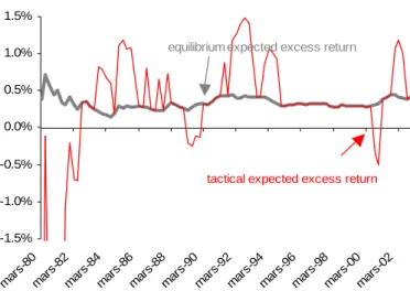
Figure 6

The US bond model: Tactical vs equilibrium expected excess returns

Figure 6 compares equilibrium expected excess returns with tactical expected excess returns, computed at the end of each quarter for the following quarter, using equation (3) minus the expected return of the money market, measured by the short-term interest rate. Clearly, tactical expected excess returns are more volatile than equilibrium expected excess returns.

III.2. The US equity model

The dividend discount model states that the fair value of a stock (or group of stocks) should be a function of the future expected dividends adjusted by a “normal” required rate of return, a mirror of a “normal” stock risk premium. Using expected earnings instead of dividends and assuming a constant long-run

payout ratio and a constant annual expected earning growth rate, we can derive the following simple dividend discount model:

k(E/P)= r+π −g (8)

where E is the one period forward looking earning yield – which determines the expected dividend – , P is the market price, k is the long-run pay out ratio, r is a risk-less rate, π is the required equity risk premium and g is the expected long-term growth of earnings.

Using (8), we can write the following statistical model for the US stock market6_:

{ t t t t t t t with LR p e ω νϕ ϕ ϕ δ µ + = + + = − + 1 value m equilibriu its yieldand earning between the deviation yield earning m equilibriu yield earningforward market 12/_{43 14243} 42 1 (9)

where the 12-month forward earning yield of the market, denoted by et+12 /pt , will be a function of the

10 year bond yield LRt, and a residual term ϕt.

-1.5% -1.0% -0.5% 0.0% 0.5% 1.0% 1.5% mar s-80 mars -82 mars -84 mars -86 mars -88 mar s-90 mars -92

We define the equilibrium earning yield as µ +

δ LRt7. ϕt

t

t

is the deviation between the market earning yield and the equilibrium earning yield. This deviation ϕ is correlated with past deviations though the coefficient ν, i.e. deviations are autocorrelated. ω is an error term iid. As in the bond case, we can calculate at any time the expected change of the earning yield:

(

(

)

)

142

(

43

)

(

14243 reversion mean 12 1 m equilibriu in change E / t t t t p LR e E∆ + = δ ∆ + ν−

)

ϕ (10)

where E and ∆ denotes the expectations operator and change respectively.

Table 4

The equity model coefficients

On the equation: et+12/-pt = µ + δ LRt + νϕt-1 + ωt Hypothesis retained for variables in equation (8) µ δ ν k π g 1980-1994 -9% 2 0.9 0.5 4% 8.5% 1995-2002 -6% 2 0.9 0.5 4% 7% mars -94 mars -96 mar s-98 mars -00 mars -02

equilibrium expected excess return

tactical expected excess return

2% 4% 6% 8% 10% 12% 14% 16% 18% 20% 1/80

We present the value coefficients retained for equation (9) on Table (4). We distinguish two periods (1980-1994 and 1995-1992) based on different assumptions about the expected nominal long-term earning growth8. As in the case of the bond model, the autocorrelation coefficient ν, has an average value of 0.99_.

We have computed the forward-looking earning yield of the US stock market using the MSCI US index universe. This forward looking earning yield is broadly a MSCI cap weighted average of forward looking earning yields provided by the I/B/E/S10

consensus data11_{. Equilibrium earning yields were}

calculated using 10-year bond yields .

Figure 7

The US market earning yield vs the equilibrium earning yield

Figure 7 compares the monthly historical earning yield of the US equity market with the equilibrium earning yield for the period January 1980-December 2002. Significant positive (negative) deviations are pointing out an undervalued (overvalued) market. This figure gives strong indication of overvaluation at end 1981, 1983-1984, October 1987 and 2000. On the other hand, the US market appears to be undervalued at the beginning of the 80’s, in 1986, 1988-1989, 93-95, September 1998 and end 2002. ___________________________________________________________________________________________

(

)

(

)

(

)

( )

4 4 4 4 4 4 4 4 4 4 4 4 3 4 4 4 4 4 4 4 4 4 4 4 4 2 14444444244444443 1 ER tactical 12 ER 12 12 12 12 12 1 -market equity market equity market equity 12 12 t t t m equilibriu t EQ t t t t t EQ t t t t t t t t e p k p e E e p e e E p e k ER p p E p e k ER p p E p d ER t t ν ϕ ⎥ ⎥ ⎦ ⎤ ⎢ ⎢ ⎣ ⎡ ⎟⎟ ⎠ ⎞ ⎜⎜ ⎝ ⎛ − + ⎟ ⎟ ⎠ ⎞ ⎜ ⎜ ⎝ ⎛ ⎟ ⎟ ⎠ ⎞ ⎜ ⎜ ⎝ ⎛ ∆ ⎟⎟ ⎠ ⎞ ⎜⎜ ⎝ ⎛ − ⎟⎟ ⎠ ⎞ ⎜⎜ ⎝ ⎛ ∆ + = ⎟⎟ ⎠ ⎞ ⎜⎜ ⎝ ⎛ ∆ + = ⎟⎟ ⎠ ⎞ ⎜⎜ ⎝ ⎛ ∆ + = + + + + + + + + (11) _______________________________________________________________________________________

The calculation of the expected total return ER of the equity market is presented in equation (11), where the expected dividend yield dt+12 / pt is

obtained through the product of the payout ratio k and the forward-looking earning yield et+12 / pt.

Note that if the market is in equilibrium, the expected return is the expected dividend yield plus the expected growth of earnings in the medium term

E(∆et+12/et+12) plus the expected change of the equity

market price following the expected change of the equilibrium earning yield – which should be rather

smooth. The tactical expected return will be the equilibrium expected return plus the difference between the observed dividend yield and the equilibrium dividend yield plus the expected change in price due to the fact that the market is in disequilibrium.

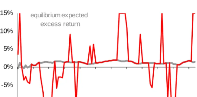
Figure 8

The US equity model – Tactical vs. equilibrium quarterly expected excess returns

11 10% -5% 0% 5% 10% 15% _{equilibrium expected} excess return

Finally, Figure 8 exhibits equilibrium and tactical expected excess returns, computed on a quarterly basis, based upon the formula (11).

Once again, this figure clearly shows the greater variability of tactical excess returns when compared with equilibrium expected excess returns.

III.3. Tactical asset allocation vs.

fundamental-driven asset allocation

In this section, we present simulations of actively managed global balanced portfolios (equity and bonds), for the US and the European markets.

The active allocation process presented in these simulations lies on the expected quarterly returns derived from the models described in the precedent section and on risk estimates for the bond and the equity markets using a historical variance covariance matrix based on 5-year monthly trailing returns.

For each of the global balanced portfolios – the US and the European portfolios, which definitions are presented below –, two simulations are performed:

a) the first one uses the equilibrium expected

excess returns for determining the fundamental-driven asset allocation. In this context, the

market price level is not taken into account, only the equilibrium expected return which is a function of the phase of the cycle and the resultant state variables of the economy. It is interesting to note that many investors use this approach when allocating in their portfolios. b) the second one uses the tactical expected

returns, resulting in the tactical asset allocation.

As we have discussed before, the price level of

the market is an important determinant of these tactical returns (impact of the observed deviation between the market price and the equilibrium price on the expected return).

The portfolios are optimised and re-balanced on a quarterly basis. An optimal portfolio is built at the end of each quarter, based on the bond and equity expected excess returns for the following quarter, under the following constraints:

a) a tracking error inferior or equal to 3% with respect to the investor’s benchmark , i.e. the investor’s long-term strategic asset allocation. b) the maximum exposure allowed is 110% (a

exposure higher than 100% may be implemented with a loan or the use of futures), the minimum exposure is 90% (a maximum of 10% of cash is allowed).

A. Simulation of an actively managed US balanced portfolio.

The benchmark – denominated in US dollars – is defined as a constant mix 60% US government bonds, with an average duration of 5, with the remaining 40% invested in equity, represented by the MSCI US equity index (no dividend reinvestment). Such a choice of a long-term strategic asset allocation is justified by a Markowitz optimization, with the hypothesis of long-term values for volatility, correlation, and expected excess returns of bonds and the stock market in the US, presented in Table 5.

Table 5

Expected excess returns and risk for the US bond and equity markets

Annualized expected excess return Annualized expected volatility Expected Bond/equity correlation US Bonds 1.1% 5% 10% US Equities 6% 16%

These long-term values are based on historical averages reported by Ibbotson and Sinquefield (2002), for the period 1926-2002 (see Table 1). The volatility of the bond market reported by this source refers to 20-year government bonds, with an average value of 9%; we modified this figure for taking into account that the duration of the bond segment in the simulated portfolio is 512_.

Table 6

The efficient frontier for the US bond and equity markets

Table 6 exhibits the Sharpe ratio of the portfolio for different constant mixes. Indeed this ratio is maximized with the mix 60% bonds and 40% equity.

The simulation period for the fundamental-driven and tactical asset allocation runs from the second quarter of 1980 until end 2002-IV.

Figure 9 exhibits the portfolio weights at the end of each quarter for the fundamental-driven asset allocation.

Since 1992, the fundamental-driven portfolio overweighs equity, reflecting the market participants’ prevailing optimism in stock markets. Prior, the stock

market is underweighted, particularly in 1988- 1989 (the market is anticipating the 1990-91 recession?).

Figure 9

US - Fundamental-driven asset allocation

0% 10% 20% 30% 40% 50% 60% 70% 80% 90% 100% 110% mar s-80 m

Globally, the portfolio moves softly. The simulation using tactical returns offers a different picture. Figure 10 exhibits the sharp reallocations at the end of each quarter for this second simulation, i.e. the tactical asset allocation, following the recommendations of the tactical signals.

The results of the two simulations are presented in Table 7. The fundamental-driven asset allocation adds 30 basis points per year to the benchmark performance (i.e. the long-term strategic asset allocation performance), while the tactical asset allocation exceeds the benchmark performance by 140 basis points per year. The information ratios are respectively 0.20 and 0.50, which illustrates the US portfolio’s performance enhancement in terms of return/risk with the use of tactical signals.

Figure 10

US - Tactical asset allocation

Table 7 ar s-82 mar s-84 mar s-86 mar s-88 mar s-90 mar s-92 mar s-94 mar s-96 mar s-98 mar s-00 mar s-02 BONDS EQUITIES

ALLOCATION Portfolio Portfolio

expected expected Sharpe BONDS EQUITIES _{volatitlity excess return} ratio

100% 0% 5.0% 1.1% 0.22 90% 10% 4.9% 1.6% 0.32 80% 20% 5.4% 2.1% 0.39 70% 30% 6.2% 2.6% 0.41 60% 40% 7.3% 3.1% 0.42 50% 50% 8.6% 3.6% 0.41 40% 60% 10.0% 4.0% 0.40 30% 70% 11.4% 4.5% 0.40 20% 80% 12.9% 5.0% 0.39 10% 90% 14.5% 5.5% 0.38 0% 100% 16.0% 6.0% 0.38 ALLOCATION Portfolio Portfolio

expected expected Sharpe BONDS EQUITIES _{volatitlity excess return} ratio

100% 0% 5.0% 1.1% 0.22 90% 10% 4.9% 1.6% 0.32 80% 20% 5.4% 2.1% 0.39 70% 30% 6.2% 2.6% 0.41 60% 40% 7.3% 3.1% 0.42 50% 50% 8.6% 3.6% 0.41 40% 60% 10.0% 4.0% 0.40 30% 70% 11.4% 4.5% 0.40 20% 80% 12.9% 5.0% 0.39 10% 90% 14.5% 5.5% 0.38 0% 100% 16.0% 6.0% 0.38 0% 10% 20% 30% 40% 50% 60% 70% 80% 90% 100% 110% mar s-80 mar s-82 mar s-84 mar s-86 mar s-88 mar s-90 mar s-92 mar s-94 mar s-96 mar s-98 mar s-00 mar s-02 BONDS EQUITIES 13

Table 7

US simulation results. Fundamental-driven and tactical asset allocation vs. the benchmark

(transaction costs are not considered)

Benchmark Fundamental driven asset allocation Tactical asset allocation Annualized volatility 8.4% 8.7% 8.8% Annualized return 10.3% 10.6% 11.7% Tracking error on benchmark 1.4% 2.6% Information ratio on benchmark 0.2 0.5

The tactical movements are mainly determined by the equity tactical returns, what can be easily understood by watching Figure 8. The price movements of the equity markets are at the origin of the opportunities presented in this simulation.

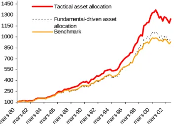
Figure 11 shows the cumulated performance of both strategies against the benchmark performance13_.

Figure 11

US – Fundamental-driven and tactical asset allocation vs. the benchmark

B. Simulation of an actively managed European balanced portfolio.

In this section, we repeat the exercise for a global balanced portfolio (equity and bonds)

denominated in Euros (French francs before 1999). The benchmark is defined as a constant mix 50% Euro government bonds, with an average duration of 5, with the remaining 50% invested in equity, represented by the MSCI European equity index (no dividend reinvestment, unhedged against the currency risk). We assume that such a choice of a long-term strategic asset allocation derives from the particular preferences and constraints of the investor.

The simulation period for the fundamental-driven and tactical asset allocation runs from the first quarter of 1989 until end 2002-IV. We computed equilibrium and tactical expected returns using the same models as in the US case. We used the French 10-year government bond rates and the European market forward earning yield based on the European MSCI index universe for calculating these returns.

Figures 12 and 13 exhibit the simulated fundamental-driven and tactical asset allocations. Particularly, we note the quite sharp movements of the fundamental-driven asset allocation at the end 1991 and 1992. This is due, on the one hand, to a decrease of the estimated risk, which lead the optimizer to raise the portfolio’s risky asset exposure at the end of 1991. The sharp reduction of the exposure to the risky assets at the end of 1992 is the consequence of the impact of the rise in short-term interest rates during the year (monetary crisis) on the equilibrium expected excess returns.

Figure 12 100 250 400 550 700 850 1000 1150 1300 1450 ma rs-8 0 mar s-82 mar s-84 m ars-86 ma rs-8 8 ma rs-9 0 mar s-92 mar s-94 m ars-96 ma rs-9 8 ma rs-0 0 mar s-02

Tactical asset allocation Fundamental-driven asset allocation

Benchmark 1980/I = 100

Europe - Fundamental-driven asset allocation

0% 10% 20% 30% 40% 50% 60% 70% 80% 90% 100% 110% BONDS EQUITIES

Figure 13

Europe - Tactical asset allocation

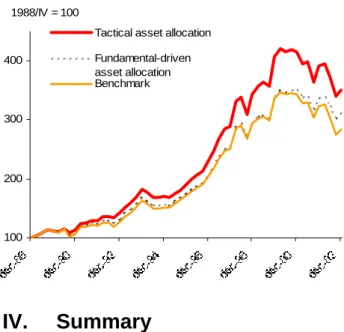
Table 8 presents the simulation results14_{. Again the}

enhancement of the portfolio’s performance using tactical returns is quite significant: the tactical asset allocation adds 100 basis points per year to the fundamental-driven asset allocation and 170 basis points to the benchmark, with a highly significant information ratio.

Table 8

European simulation results. Fundamental-driven and tactical asset allocation vs. the benchmark (transaction costs are not considered)

Benchmark Fundamental driven asset allocation Tactical asset allocation Annualized volatility 10.6% 9.3% 10.3% Annualized return 7.7% 8.4% 9.4% Tracking error on benchmark 1.8% 2.2% Information ratio on benchmark 0.4 0.7 Figure 14

Europe – Fundamental-driven and tactical asset allocation vs. the benchmark

IV. Summary

Different levels of asset allocation can be defined, which will depend mainly on the information used in the allocation decision process . More precisely, we made the distinction between:

1) long-term asset allocation: the benchmark of an investor, function of the investor constraints and his long-term vision for returns and risk of the financial assets.

2) the fundamental-driven asset allocation, conditional on the equilibrium expected returns in the medium term. Typically defined for a period of around 5 years, these returns are the mirror of the “normal” expected premiums of the financial assets, consistent with the economic cycle and/or structural changes of the economic/financial environment. By their nature they are persistent, resulting in slow changes in the asset allocation in the medium-term.

3) the tactical asset allocation, conditional on tactical asset returns. Tactical asset returns are typically defined for the short-term (3/6 months) and are mainly the consequence of important deviations between the market price and the equilibrium price of the financial asset, i.e. periods of significant market over/under valuation. Tactical asset allocation exploits short-term transitory mispricing in the markets.

0% 10% 20% 30% 40% 50% 60% 70% 80% 90% 100% 110% BONDS EQUITIES 100 200 300 400

Tactical asset allocation Fundamental-driven asset allocation Benchmark 1988/IV = 100

We simulated expected returns for the US bond and stock markets since 1980, using valuation models issued from the financial theory (the Expectation Hypothesis theory and the Dividend Discount Model) We illustrated the three levels of asset allocation defined above through a simulation of an actively managed global balanced portfolio (equity and bonds) denominated in US dollars, for the period 1980-2002. We repeated the exercise for a global balanced portfolio denominated in Euros, for the period 1989-2002. Both simulations underline the importance of the fundamental-driven asset allocation, and, overall, the tactical asset allocation as sources of value.

References

Ang, Andrew and Geert Bekaert, 2003, “The Term Structure of Real Rates and Expected Inflation”, working paper, Columbia University and NBER Buraschi, Andrea and Alexei Jiltsov, 2002, “Is Inflation Risk Priced?”, working paper, London Business School.

Campbell, John Y., Andrew W. Lo and A. Craig MacKinlay, 1997, The Econometrics of Financial

Markets, Princeton University Press, Princeton, New

Jersey .

Consensus Forecasts, October 2003.

Dahlquist, Magnus and Campbell R. Harvey, 2001, “Global Tactical Asset Allocation”, Working paper 57, Duke University.

Fama, Eugene, 1990, “Term-Structure Forecasts of Interest Rates, Inflation, and Real Returns”, Journal

of Monetary Economics 25, 59-76.

Gordon, M., 1962, The Investment, Financing and

Valuation of the Corporation, Irwin, Homewook, IL.

Greenspan, Alan, 2002, “Opening Remarks on the Federal Reserve Bank of Kansas City Economic Policy Symposium”, Economic Review 4th quarter 2002, Federal Reserve of Kansas City, 5-13.

Hamilton, James D., 1994, Time Series Analysis, Princeton University Press, Princeton, New Jersey. Hartpence, Maria and Jacques Sikorav, 1996, “Tactical Asset Allocation: The Quest for Value”,

Quants 21.

Homer, Sydney, and Richard Sylla, 1991, A History

of Interest Rates, 3rd edition, Rutgers University

Press.

Hunt, Lacy and David Hoisington, 2003, “Estimating the Stock/Bond Risk Premium”, The Journal of

Portfolio Management, Winter 2003.

Haugen, Robert, 1995, The New Finance: The Case

against Efficient Markets, Prentice Hall, Englewood

Cliffs, New Jersey.

Ibbotson, Roger and Rex Sinquefield, Stocks, Bonds,

Bills and Inflation Yearbook 2002, Ibbotson

Associates Inc., updated annually.

International Financial Statistics, IMF, various

issues.

Merton, Robert C., 1973, “An Intertemporal Capital Asset Pricing Model”, Econometrica 41, 867-887. Markowitz, Harry, 1952, “Portfolio Selection”,

Journal of Finance 7, 77-91.

Mills, Terence C.,1993, The Econometric Modelling

of Financial Time Series, Cambridge University

Press.

Mills, Terence C., 1991, “Equity Prices, Dividends and Gilt Yields in the UK: Cointegration, Error Correction and “ Confidence ” ”, Scottish Journal of

Political Economy 38, 242-55.

Shiller, Robert J., 2001, Irrational Exuberance, Princeton University Press.

Schwert, William, 1990, “Indexes of US Stock Prices from 1802 to 1987”, Journal of Business vol. 63, n° 3.

Siegel, Jeremy and Peter Bernstein, 1998, Stocks for

the Long Run, 2nd edition , McGraw Hill Professional

Publishing.

Siegel, Jeremy, 2001, “Historical Results 1”,

Proceedings from The Equity Risk Premium Forum,

AIMR, November 8, 2001.

Tong, Howell, 1983, “Threshold Models in Non-linear Time Series Analysis”, Lecture Notes in

Statistics 21, Berlin: Springer-Verlag.

Endnotes

1 _{Indeed, interest rates, like inflation, are lagging}

indicators of the economic cycle, and even at the beginning of the expansion period interest rates may remain low for a while as long as inflation keeps to a low level.

2 _{The Expectation Hypothesis (EH) model is based}

on the belief that the whole term structure is determined by market expectations about future spot interest rates. In one of its versions, the EH model states that the period yield Ynt will average the

expected return of rolling over one period bonds for n periods, plus a premium τ, which can be constant or time varying over time:

(

1+ ,

)

= t

(

(

1+ 1,t+ t

)(

1+ 1,t+1+ t+1

) (

1+ 1,t+n−1+ t+n−1

)

)

n t n E Y Y Y Y τ τ _K τ 17

where Ynt is the period yield of an n-period bond,

which should equal – under the EH – to the geometric average of the expected return from rolling over one period bonds for n periods plus a risk premium τ. A model such as the one defined in equation (1) is “projecting” market expectations about future short rates and risk premiums on the spot short rate SRt and the expected inflation INFt. 3 _{Our own calculations of long bond and money}

market returns, using 10-year government bond monthly yields and 3-month Treasury Bills for the period January 1957 to December 2002 (source: IMF International Financial Statistics), show an average compound annual excess return for long bonds of 1.1% (6.9% for bonds vs. 5.8% for T-Bills), while the average of the difference of long bond yields and T-Bill rates was 1.4%. According to Ibbotson and Sinquefield (2002, see Table 1), the compound average annual US government bond return for the period 1926-2002 reached 5.45% against 3.79% for monthly Treasury Bills, giving an historical bond excess return of 1.66% (though these figures are based upon 20-year government US bonds), while Siegel (2001) reports a premium of 1.1% for the period 1871-2001 (see Table 1). Using these results concerning historical bond premiums, we may assume the long-run required premium of 10-year government bond yields on the risk-free asset (monthly T-Bills) to be around 1.3%/1.5% . On the other hand, the inflation risk premium, i.e., the part of the bond premium which is due to the uncertainty of expected inflation, have been estimated by some experts to be 60 basis points on average (Buraschi, Jiltsov, 2002), while others estimate the inflation risk premium to be around 100 basis points (for a 5-year horizon, Ang and Bekaert, 2003), with a high degree of variation following the level/volatility of inflation. Another stylized fact about the term structure of interest rates reported by experts is that “…long rates rise less than short rates during business expansions and fall less during contractions…” (Fama, 1990).

4 _{We have calculated the US equilibrium long}

rate and the implied equilibrium required risk premium based upon the coefficients of the model for a 10-year bond using historical data for different periods and data issued from market consensus expectations concerning inflation and short rates. These values are exhibited in the following table.

Long rate, equilibrium long rate and equilibrium risk premium implied by the bond model

Average values

Short rate Inflation rate Equilibrium long rate Equilibrium required risk premium Observed long rate Consensus expectations 4.0% 2.3% 5.4% 1.4% 5.4%1 Ibbotson (1926-2002) 3.8% 3.1% 5.3% 1.5% 5.8% IMF (1954-2002) 5.6% 5.7% 7.4% 1.8% 7.0% Bloomberg, OECD (1980-2002) 6.4% 4.2% 7.8% 1.4% 8.1% Average 5.0% 3.8% 6.5% 1.5% 6.6%

1 _{corresponds to the long-term expected long rate}

The line “Consensus expectations” calculates the equilibrium long rates and required risk premium using long-term consensus expectations about short rates and inflation (for 2009/2013, this data was published in the October 2003 Consensus Forecast) . The “observed long rate” in this case corresponds to the long-term consensus expectation about long rates. We can see that the long rate expected by the market consensus and the equilibrium long rate calculated by the model (using consensus expectations about short-rates and inflation) are identical in this case. The other lines exhibit calculations using Ibbotson data for the period 1926-2002, IMF data for 1954-2002 and Bloomberg/OECD data for the period 1980-2002. We can see that the average long rates of those periods are quite close to the equilibrium long rate implied by the model.

5 _{The ρ coefficient was allowed to vary at each}

period t, as a function of the magnitude of disequilibria at period t-1, mean reversion being stronger the higher the disequilibrium value – measured in standard deviations –, and absent for very low disequilibria. This approach is based on the use of a threshold autoregressive model (TAR), see Tong (1983). The values of the ρ coefficient in the bond market model are the following :

Fundamental Tactical

Year Bench driven asset

asset alloc allocation

performance Surperformance performance Surperformance

1980 16.2% 14.4% -1.8% 17.9% 1.6% 1981 0.4% 1.5% 1.0% 2.0% 1.5% 1982 22.7% 22.7% 0.1% 20.8% -1.9% 1983 9.7% 10.1% 0.4% 8.3% -1.4% 1984 8.4% 8.3% -0.1% 11.5% 3.0% 1985 23.1% 21.9% -1.2% 24.9% 1.8% 1986 17.1% 15.9% -1.2% 16.8% -0.3% 1987 2.4% 3.0% 0.5% 12.9% 10.5% 1988 10.2% 9.9% -0.3% 10.4% 0.3% 1989 19.7% 18.8% -0.9% 19.0% -0.8% 1990 2.2% 2.7% 0.6% 2.8% 0.7% 1991 18.3% 17.6% -0.7% 18.5% 0.2% 1992 7.2% 7.9% 0.7% 7.8% 0.6% 1993 11.3% 11.3% 0.0% 10.8% -0.4% 1994 -2.2% -2.4% -0.2% -1.6% 0.7% 1995 25.2% 27.8% 2.7% 27.4% 2.3% 1996 9.3% 11.2% 1.9% 12.9% 3.6% 1997 18.9% 21.9% 3.0% 18.2% -0.7% 1998 18.6% 21.4% 2.8% 24.3% 5.7% 1999 6.5% 8.5% 2.0% 11.8% 5.3% 2000 2.0% -0.4% -2.4% 3.6% 1.6% 2001 -1.6% -3.1% -1.6% -4.3% -2.7% 2002 -3.2% -2.0% 1.2% -2.2% 1.0% If |ut-1| =< σu 1 If σu < |ut-1| =< 2 σu 0.9 If |ut-1| > 2 σu 0.8

6 _{This approach is similar to the one used by the}

Federal Reserve (Greenspan, 2002).

7 _{Note that the discount or required rate of return is}

represented by the bond yield plus an equity risk premium over the bond yield. The constant term µ embodies the expected long-term earning growth and the long-run required risk premium of the equity market on the bond market multiplied by the inverse of the long-term payout ratio k. The coefficient δ is precisely the inverse of the payout ratio k.

8 _{These values are based on the assumption of a}

expected payout ratio of 0.5, which corresponds to a long-run observed average (based on Shiller, 2002). We assume a long run required risk premium over bonds of 4% (based on Ibbotson and Sinquefield, 2002, and Shiller, 2002, see Table 1), the expected long-term earning growth is assumed higher before 1995, as it includes higher inflation expectations than after that year. The expected long-term earning growth figures are based on the historical average growth of the earning per share of the S&P index following Shiller (2002), which reached almost 4% for the period 1946-1980 in real terms, and 8.4% in nominal terms. For the period 1871-2002, average earning growth was significantly lower (1.3% in real terms), but we think that post-war values were nearer from the investor’s expectations during the 80s and the 90s about future corporate productivity and profits.

9 _{The coefficient ν is time varying and depending on}

the level of disequilibria at t-1.

ν

If |ϕt-1| =< σϕ 1 If σϕ < |ϕt-1| =< 2 σϕ 0.9 If |ϕt-1| > 2 σϕ 0.8

10 _{I/B/E/S is one of the leading companies which ,}

among other things, collects earnings expectations

data from more than 4000 analysts, covering more than 27,000 US an international companies.

11 _{This calculation was made since 1987. For}

problems of data availability, we calculated the forward looking US earning yield before 1987 using the backward looking MSCI US earning yield, multiplied by (1+g).

12 _{It is interesting to note that the values}

reported in Table 5 in terms of volatility are quite close to the averages registered for the period 1998-2002.

13 _{US portfolio simulation details}

14 _{European portfolio simulation results}

Fundamental Tactical

Year Bench driven asset

asset alloc allocation

performance Surperformance performance Surperformance 1989 12.2% 10.9% -1.4% 11.8% -0.4% 1990 -5.5% -1.2% 4.3% 1.0% 6.5% 1991 13.5% 13.3% -0.2% 14.9% 1.4% 1992 5.8% 7.4% 1.6% 10.3% 4.5% 1993 29.0% 27.8% -1.3% 27.7% -1.3% 1994 -7.8% -8.3% -0.5% -7.2% 0.5% 1995 13.1% 12.3% -0.8% 12.8% -0.3% 1996 18.5% 17.9% -0.6% 19.7% 1.2% 1997 23.6% 23.3% -0.3% 26.1% 2.5% 1998 16.7% 16.2% -0.5% 19.0% 2.4% 1999 14.7% 15.1% 0.4% 18.4% 3.6% 2000 2.2% 2.9% 0.7% 2.0% -0.2% 2001 -5.7% -4.0% 1.7% -5.5% 0.2% 2002 -12.4% -7.6% 4.9% -10.6% 1.8%